Advanced ICP-MS methods for examining the stability of silver nanoparticles in natural waters

(1)

ADVANCED ICP-MS METHODS FOR EXAMINING THE STABILITY OF SILVER NANOPARTICLES IN NATURAL WATERS

By

(2)

ii

A thesis submitted to the Faculty and the Board of Trustees of the Colorado School of Mines in partial fulfillment of the requirements for the degree of Master of Science (Chemistry).

Golden, Colorado

Date______________________

Signed: _________________________________ Thomas Joseph Gately

Signed: _________________________________ Dr. James F. Ranville Thesis Advisor Golden, Colorado Date__________________________ Signed: _________________________________ Dr. David T. W. Wu Professor and Head Department of Chemistry and Geochemistry

(3)

iii

ABSTRACT

The rapid growth of nanotechnology, specifically the incorporation of engineered nanoparticles (ENP’s) into various products, will almost certainly lead to their release into the environment. Silver nanoparticles (nano-Ag) have seen widespread use in consumer products as a result of their antimicrobial properties. Silver ion (Ag+), is known to be toxic to a large variety of organisms, especially aquatic species. The release of Ag+ from nano-Ag under relevant environmental conditions is not currently well understood, as many studies use unrealistically high concentrations. This is in part due to limitations in the techniques used to detect and characterize ENP’s. Using Single Particle Inductively Coupled Plasma Mass Spectrometry (SP-ICP-MS), a newly developed method to examine ENPs we are able to detect and quantify both nano-Ag and Ag+ at part per trillion concentrations, considered a realistic environmental level. In a collaborative study with the Trent University, PVP-coated 50 nm nano-Ag particles were introduced into several mesocosms within a lake. Their fate (particle number, dissolution) was monitored by a number of methods including SP-ICP-MS, FFF-ICPMS, and total Ag analysis. Before the experiment could proceed a preservation method was needed to allow sample transport from the Ontario Lake to the lab in Colorado. Flash freezing using liquid nitrogen was found to be an effective method for preserving the particles that there was minimal change to the particle size and number. The samples were stored at -80˚C until the time of analysis. 60 nm PVP capped particles were initially found to be 58.3 ± 5.3 nm and the flash frozen particles were found to be 58.4± 5.2 nm. A series of lab experiments were also performed using lake water in which the

(4)

iv

stability of nano-Ag particles was examined. The particles were found to decrease in diameter from 50 nm to 36 nm over the course of seven days. Particle number also decreased over the course of the experiment illustrating that further work on

methodology is required. Typical decreases in particle number were on the order of 60% over the course of a week. The rate of particle loss/transformation was

significantly slower when lake waters were filtered suggesting a role for other

suspended sediments or biota in the process. Sterilization using autoclaving provided further evidence for the role of biota but results showed complex behavior depending on the methods used (e.g. filtration and autoclaving). This study further demonstrates the utility of SP-ICP-MS to detect, quantify and characterize ENPs, but further work is needed to fully understand the processes controlling nano-Ag stability in aquatic environments.

(5)

v

LIST OF FIGURES

Figure 1-1: A 500 ppt dissolved silver standard on SP-ICP-MS ... 7

Figure 1-2: A 60 nm particle standard in SP-ICP-MS. ... 10

Figure 2-1: The concentration effects of silver nanoparticles on dissolution ... 13

Figure 2-2: The dissolved peak vs. particle silver. ... 15

Figure 2-3: A comparison of fresh and one week old silver nanoparticles... 17

Figure 2-4: Particle dissolution in a natural water and DI water. ... 19

Figure 2-5: A comparison of stabilized and fresh nanoparticles. ... 22

Figure 2-6: Effect of -10 ˚C freezing on nanoparticle size 60nm PVP capped particles. 24 Figure 2-7: Effect of liquid nitrogen freezing on particle size of 60 nm PVP capped particles. ... 25

Figure 3-1: The samples from the first week of the lake experiment showing particle dissolution and loss ... 30

Figure 3-2: The decrease in particle diameter over time for replicate mesocosms.. ... 30

Figure 3-3: The mass particulate and dissolved silver over time obtained from integrating the SP-ICP-MS signal. ... 32

Figure 3-4: Particle diameter and number over time for long term samples showing dissolution and particle loss.. ... 32

Figure 3-5: The decrease in particle mean diameter and number over time. ... 33

Figure 4-1: The % change in 107Ag counts for a 500 ppt dissolved silver diluted in lake water and 10% nitric acid as compared to 2% nitric acid.. ... 37

Figure 4-2: The calibration slopes for dissolved silver in lake water, DI water, 2% nitric acid and 10% nitric acid immediately after preparation. ... 37

(9)

ix

Figure 4-3: The calibration slopes for dissolved silver in lake water, DI water, 2% nitric

acid and 10% nitric acid prepared three days prior to analysis. ... 38

Figure 4-4: The percent change in counts over three days of dissolved silver standards relative to their respective matricies. ... 39

Figure 4-5: Comparison of initial of 60 nm PVP capped Ag to particles recovered from container by sonication. ... 41

Figure 4-6: The measured counts for silver removed by subsequent acid rinses of the container. ... 43

Figure 4-7: The loss in particle diameter of 60 nm PVP coated particles after one week in natural water and DI water showing similar behavior. ... 45

Figure 4-8: The loss in particle diameter of 60 nm PVP coated particles after one week in filtered natural water and DI water showing slower dissolution in filtered lake water. 46 Figure 4-9: The effects of sodium azide on particle dissolution in filtered lake water. ... 47

Figure 4-10: The effects of sodium azide on particle dissolution in filtered lake water. . 48

Figure 4-11: The effects of sodium azide on particle dissolution in filtered lake water. . 50

Figure 4-12: The loss of particulate silver in terms of normalized mass over time. ... 52

Figure 4-13: The loss of particles in lake water over time in the lab re-creation ... 53

Figure 4-14: The loss of diameter in lake water from the particles over time ... 54

(10)

x

LIST OF TABLES

Table 4-1: The results from the laboratory silver tracking... 43

Table A-1: Water Chemistry for filtered and unfiltered samples ... 63

Table A-2: Water chemistry at the lake during sampling: ... 64

(11)

xi

ACKNOWLEDGMENTS

There are a great many people I would like to thank during my time here at Mines. Dr. Jim Ranville has been my advisor through my undergraduate and graduate career. Along the way he has been an advisor, professor and boss to me. He has continued to drive me to do bigger and better things. Dr. Tom Wildeman has also been continually pushing me here at Mines since I began working on the ICP’s the summer of my freshman year. I am also extremely appreciative for Dr. Chris Higgins giving me advice and guidance while Jim was away on sabbatical. I would also like to thank my supportive colleagues in the research group especially Denise Mitrano and Robert Reed for helping acquaint me with the SP-ICP-MS and the data processing that came along with it. I would also like to thank Val Stucker and Manuel Montaño for keeping the ICP-MS operational. I would also like to thank Trent University and Lindsay Furtado and Chris Metcalf for organizing and performing the lake experiment. I am also very grateful for all of the people that have passed through the research group and helped make my experience what it was.

Outside of Mines there is also a multitude of people I would like to thank. First and foremost I would like to thank my parents for their encouragement, support, and understanding throughout my time in college. I am also thankful for the rest of my family for their support in my endeavor as well. I would like to thank my friends that have stuck around and made my college experience what it was. I would also like to thank all of my science and math teachers for making me wonder and want to know more, especially Mrs. Davidson and Mrs. Hyde for getting me hooked on chemistry.

(12)

xii

Finally I would like to thank Kristina Lucas for her support, dedication and ability to listen to me talk about my research for hours on end.

(13)

1

CHAPTER 1 :

INTRODUCTION

The use of nanotechnology is not new. Nanoparticles have been found to have been used in ancient Egypt, and more widely in medieval Europe, predominantly in artwork. In 1857 Faraday was able to make gold and silver nanoparticles intentionally [1]. These had no immediate uses though and nanotechnology was largely forgotten about. On December 29, 1959 Richard Feynman delivered a lecture entitled ‘There is Plenty of Room at the Bottom’ which made the case for nanotechnology. In his speech he said that designing a material or chemical from the ground up allowed for it to better serve its intended purpose. The term nanotechnology was not coined until years later by Norio Taniguchi [2]. During the 1980’s there was a rapid increase in research in the field of nanotechnology. Fullerenes, which later won the Nobel Prize, were invented in 1985. Other advancements in the 1980’s include the discovery of carbon nanotubes and the advancements in electron microscopy which allowed nanomaterials to be seen. In 1986 K. Eric Drexler wrote the book Engines of Creating: The Coming Era of

Nanotechnology which is thought to have thrust nanotechnology into the limelight.

Nanotechnology began to draw more and more attention in the scientific community. In 1989 Science began printing a journal Nanotechnology, and in 1991 a special issue on nanotechnology was published. In 2000 then President Bill Clinton delivered a speech at Cal Tech proposing large scale funding to nanotechnology research. In 2003

(14)

2

Development Act into law authorizing billions of dollars into nanotechnology research [3].

Nanotechnology is generally defined as the control of matter at dimensions between approximately 1 to 100 nanometers where unique phenomena arise and allow for novel applications. The main properties that are manipulated at this size are structure and shape. Nanoparticle composition can be organic, inorganic or a combination thereof. Nanoparticles represent a unique area with their properties; they do not exhibit the solid state properties of bulk material, nor do they exhibit the properties of quantum

mechanics, it is a blend between the two. Applications of nanoparticles are wide ranging; things from sunscreen and soap to baby carriages and clothes currently exist with many other promising applications in the works. The chemistry of these particles is widely studied but it is also important to understand the impact of this new science. Generally the impact of new research is not understood until years later. DDT and Thalidomide are just two examples of chemicals that had ramifications later.

1.1 Nano silver applications

Silver has long been used for its antimicrobial properties. Nano silver’s primary use is for these antimicrobial properties. The exact mechanism of nanosilver’s toxicity to microbes is still being studied but it is believed that the silver ion is responsible for toxicity, not the particles themselves. The nanoparticle silver simply delivers the silver to the site where it is needed [4]. Silver has an advantage over other antimicrobial chemicals as it is incredibly hard to microbes to become resistant to it. Potential

(15)

3

silver receives the most attention of all current nanomaterials and wide gaps still exist in the knowledge of nanosilver [6]. The promise of nanotechnology is set to have wide ranging implications. Currently the market is experiencing rapid growth and is projected to be over a trillion dollar industry before the end of the decade [7]. The current rapid growth of the use of silver is generally thought to need more attention in order to

prevent adverse effects later on [8]. Most products that use nanosilver capitalize on its antimicrobial properties; examples include paint, bandages, socks, food containers, soap, and bed sheets amongst others. When these products are washed or thrown away some of the nanoparticle silver will be removed and released into the environment [9]. The fate of these particles and whether they are toxic as particles still is the focus of much study.

1.2 Adverse effects of silver in water

In recent history the major source of silver in water has been from photographic uses. In recent years though the increase of digital photography has decreased the use of film cameras and the amount of silver discharged into natural waters. This silver pollution has had adverse effects on various biomes [10]. There is still a lack of

understanding as to how silver nanoparticles, and other facets of nanotechnology affect the environment though research in the area is increasing [11]. The toxicity of silver in its aqueous form has been widely studied in a variety of aquatic organisms and is found to be primarily toxic in the Ag+ form of silver. Nanosilver does not appear to be toxic to animals in its particle form, the dissolution of the particles is the primary reason for the toxicity of silver nanoparticles [12]. Few studies have been performed at

(16)

4

environmentally relevant concentrations and this obscures whether or not long term chronic toxicity may prevail [13]. The dissolution rate of these silver nanoparticles varies widely however. Contributing factors include the surface coating, water chemistry, dissolved oxygen, and a plethora of other factors [14].

The silver ion is toxic to a wide range of organisms, predominantly bacterial and aquatic organisms. The mechanism for silver toxicity is not completely understood but it is generally accepted that free silver ions or reactive oxygen species (ROS) are the reason for the toxicity. ROS include singlet oxygen (O), superoxide (O2-), hydrogen peroxide (H2O2), and hydroxyl radical (OH-). In bacterial cells it is thought that the cell is attacked in three ways, first the silver can bind to and ultimately lyse the cell wall,

second the silver can bind to and disable enzymes within the cell, finally the silver will bind with DNA making further replication or transcription of the DNA nearly impossible [15]. Once within the cell the silver is believed to create reactive oxygen species which further attacks the cell [16]. ROS occur naturally in small levels as part of aerobic respiration. Recent studies have shown that it is likely that the ROS are the primary reason for cell death [17] but this ultimately remains disputed. The effectiveness of nanosilver on differing types of bacteria is also uncertain. Gram positive and gram negative bacteria have very different cell walls which can affect how nanosilver or silver ions interact with the cell. Most toxicity tests are done with E. coli bacteria. Further study of the effects of nanosilver on different bacteria is needed [18].

The toxicity and mechanisms of action for the toxicity of nanosilver in aquatic organisms is not as well understood. There are two primary types of toxicity in organisms. Acute toxicity is a single large dose of a chemical that causes toxicity.

(17)

5

Chronic toxicity is a long term small exposure to a chemical or substance. In

environmentally relevant concentrations chronic toxicity is likely to be a greater concern as the dose level will be low [19]. The toxicity of silver nanoparticles on aquatic

organisms is not as well studied as the bacterial mechanisms. Some studies have shown limited chronic toxicity of silver nanoparticles in aquatic organisms as well as reproduction difficulties but further studies are needed to conclude of this truly happens at environmentally relevant concentrations [20]

In natural waters silver is generally at a low concentration. Natural waters also tend to have compounds that reduce the toxicity of silver as well. Complexation of ions or dissolved organic carbon (DOC) with silver reduces the free silver ions and thus its toxicity. Competing cations also reduce the toxicity of silver ions in solution by competing for sights where a silver ion may bind to an organism [15].

1.3 Detection of silver nanoparticles (SP-ICP-MS)

A wide variety of methods exist for detecting and characterizing nanoparticles. Scanning Transmission Electron Microscopy (STEM) is one such method that allows for an image to be seen of the actual particles. This is powerful in some regards as the specific size and shape of the particle can be seen. This has many drawbacks too however as sample preparation can be quite extensive and alter the sample, the

instrument is expensive, the concentration of the particles is not possible to obtain, and only a small portion of the actual sample is actually looked at. This technique is useful for characterizing nanoparticles but it needs to be used in corroboration with other techniques in order to fully characterize the nanoparticles.

(18)

6

Another popular technique used to characterize nanoparticles is dynamic light scattering (DLS). This technique allows for a general size distribution to be obtained. DLS works by using a laser that is shone through a liquid. The particles will reflect a portion of the beam of light. The detector is at an angle relative to the laser. Using the Stokes-Einstein equation for Brownian motion particle size distribution can be calculated from the reflected (backscattered) light. The DLS is convenient as it is easy to use and gives the mean and standard distribution of the particle distribution. DLS has detection size limitations, both in diameter and resolution of particles of different sizes, a very high (mg/l) concentration requirement and potential for interference from other particles or things in solution. DLS can be used to find the Zeta potential of particles too if it is coupled with a charged electrode. This will allow the surface charge to be found [21].

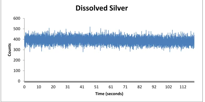
ICP-MS can be used to find the total concentration of an element in a dissolved solution. ICP-MS works by nebulizing a solution, sending it through a spray chamber where droplets larger than 2 µm do not pass through, and then using an argon plasma to ionize the atoms. The stream of ions goes through a series of cones where the majority of the ions do not pass through. The mass spectrometer of the instrument is kept under high vacuum along with the detector. A series of ion lenses focuses the ion stream into a mass spectrometer. A mass spectrometer, in our case a quadruple, is connected after the ion optics and the ions are separated by mass using varying magnetic field strength. At any given time only one charge to mass ratio will pass through the quadruple and into the detector. This will give results in counts which can be converted to concentration using a calibration slope [22]. This does very little to tell us about the nanoparticle though. Figure 1-1 on the next page shows a 500 ppt 107 Ag

(19)

7

dissolved standard. The dwell times are 10 ms long. The average is taken over the entre sample and used for the calibration.

Figure 1-1: A 500 ppt dissolved silver standard on SP-ICP-MS

Single Particle ICP-MS (SP-ICP-MS) is a technique that requires very little modification to an ICP-MS to work. This method works by changing the dwell time from several seconds for a normal SP-ICP-MS to 10 ms. This change in the dwell time allows us to observe discrete events. The dissolved standards will appear approximately the same as it would in a regular ICP-MS. A nanoparticle sample will show up as pulses over a nearly blank background (Figure 1-2). The intensity of this pulse is related to the mass of the particle and therefore its volume.

The process begins with a dissolved gold calibration slope. This concentration slope must be converted to a mass. A gold nanoparticle of a known diameter is run and a nebulization efficiency is calculated for the particle. The nebulization efficiency is the

0 100 200 300 400 500 600 0 10 20 31 41 51 61 71 82 92 102 112 Co u n ts Time (seconds)

Dissolved Silver

(20)

8

amount of the sample that makes it from the nebulizer into the quadruple for analysis [23]. The mass per event is calculated from the equation 1.1.

Where Me is the mass of the event, Ne is the nebulization efficiency, Fr is the flow rate, Dt is the dwell time, and C is the concentration. This converts the concentration slope to a mass slope for use in the next formula. The mass of the individual particle is then calculated from equation 1.2.

Where Ip is the intensity of the pulse, mp is the mass of metal in the particle, IBgd is the intensity of background, Ip is the intensity of the pulse,η is the ionization

efficiency, m is the slope of the calibration curve and fa is the mass fraction of the

analyte in the sample. By taking the mass of the nanoparticle and assuming a spherical geometry we are able to rearrange the equation of a sphere to obtain equation 1.3.

(1.1)

(1.2)

(21)

9

Where d is the diameter of the particle. This is not the hydrodynamic diameter but the diameter of the metal in nanoparticle. After doing this process with a gold nanoparticle of a known diameter a silver calibration slope is then recorded using the found nebulization efficiency. A test particle of a known diameter is run and the calculated diameter is checked against the known diameter [24]. In order to produce the graphs used to compare results the data is binned, usually in sets of 2 nm, and a histogram is produced. The histograms can be overlaid allowing for a direct

comparison. The raw data obtained from a SP-ICP-MS analysis can be seen in Figure 1-2. The bulk of the readings in the sample are the same as background readings. A pulse occurs in the data around five percent of the time. The concentration of particles for analysis in SP-ICP-MS usually needs to be in the part-per-trillion range. If the solution contains too many particles the instrument will show a doublet peak. This means that two particles entered the plasma during a single dwell time. A typical doublet peak will show up around 1.25 times what the diameter of the initial particle.

Another advantage of SP-ICP-MS is that the particles and background can be separated from each other which allows for a quantification of dissolved and particulate silver [25]. This can be particularly useful as dissolved silver is known to be toxic to organisms. It is also slows us to track the fate of the particles. Aggregated particles will show up as a larger particle while a dissolved particle will show up smaller and as an increase the background. The technique has been verified to size various nanoparticles accurately in a variety of conditions [26]. SP-ICP-MS can be connected to other

separation methods such as a method of field flow fractionation (FFF) in order to give better particle resolution [27]. This particular technique was not used during this

(22)

10

experiment but it may help later on for more accurate tracking of particles. The major down side of the technique is it required higher particle concentrations in order to obtain a size distribution. In the part per trillion levels the distribution is too broad in order to get an accurate reading.

Figure 1-2: A 60 nm particle standard in SP-ICP-MS.

Most of the readings are less than 5 in this graph. The peak height corresponds to particle diameter by relating the pulse intensity to a mass, then assuming a spherical

geometry

1.4 Format of this Thesis

The general outline of this thesis is as follows: the research began with the issue of transporting particles from lakes to the lab at Colorado School of Mines. This is covered in Chapter two. Chapter three contains the procedures and results from the lake

experiments done with the cooperation of Trent University. Chapter four contains laboratory experiments that attempt to enhance our understanding of the fate of the

0 50 100 150 200 250 300 0 10 20 31 41 51 61 71 82 92 102 112 Co u n ts Time (seconds)

60 nm Particle ICP-MS-SP

(23)

11

particles in natural waters. Chapter five contains the conclusions and potential future work that can be continued on in future projects.

(24)

12

CHAPTER 2 :

THE FATE OF NANOPARTICLES AT LOW CONCENTRATIONS

Silver nanoparticles have received much research attention due to the toxic nature of silver in the environment. The majority of silver nanoparticle toxicity test have been done at relatively high concentrations however [28]. If silver is released from human sources it is likely to be in small quantities and then will be further diluted when it mixes with the rest of the sewer system. If the silver nanoparticles make it to a natural water system they will be in extremely small quantities, generally on the order of parts per trillion (ppt). Figure 2-1 shows the difference of dissolution of particles at two different concentrations. The high concentration is at approximately 50 ppb while the low concentration is at 50 ppt. The difference in dissolution over the course of a week is quite immense. The average diameter decreased by approximately 10 nm. Given the cube term of the radius in the volume of a sphere a change in diameter from 60 nm to 50 nm represents approximately a 31% loss of silver by mass. If the original solution started at 50 ppt after a week 15.3 ppt of the silver would be available as a silver ion. Several studies have been performed on particles at part per billion levels in natural water or more concentrated. The results of these studies have shown both aggregation and dissolution of the particles. The rate of each depended on a wide variety of factors from ion concentrations and DOC concentration to temperature and sunlight levels [29]. Experiments in the lab began with a simple deionized water and silver nanoparticle solution and became more complex as experiments progressed.

(25)

13

Figure 2-1: The concentration effects of silver nanoparticles on dissolution The red in the histogram was 60 nm 50 ppb particles after one week while the black was at 50 ppt after one week. The particles were 60nm PVP capped silver particles.

2.1 Introduction

At the Trent University in Peterborough Canada our colleagues were planning a lake experiment where silver nanoparticles would be added to mesocosms in a lake at the Experimental Lakes Area (ELA) in Ontario. Samples were taken at various time intervals for four weeks. The samples would then be sent from the lake in Canada to our lab for SP-ICP-MS analysis. Given how silver nanoparticles can dissolve and aggregate over time even overnight shipping or transportation to the nearest lab could have a significant impact on many time points. It became important to develop a preservation method for the transport of the samples from the lake to the lab. This

(26)

14

method would have to prevent any reactions from occurring during the trip to the lab. There were three primary methods that were examined for preserving the particles. The first was a chemical method of preservation. Nanoparticles are usually coated with a chemical that aids in preventing aggregation and dissolution. Many different chemical coatings exist but the most widely used are PVP, citrate, and tannic acid. Simply adding a chemical to the solution to keep the particles in solution would be very

advantageous in field work as it is straightforward, cheap and easy to accomplish. The second option was a method of freezing. Freezing particles is generally not

recommended as it may damage or otherwise change the shape and size of the nanoparticle. Several different types of freezing are available with the two primary methods being flash freezing and standard freezing. Flash freezing is typically done with liquid nitrogen. The freezing process happens so quickly that the water molecules cannot form their typical structure as they solidify. The main disadvantage of freezing samples is the equipment needed in the field to freeze the samples is quite extensive and can boil off or sublimate if it is not used in a timely manner. The samples must also be transported frozen which can be problematic for long journeys. Finally oxygen is thought to be the primary reason that nanoparticles dissolve in solution. If the samples are made anoxic it is likely that the particles would stay in solution for the trip. This process also has the advantage of easy storage but it would be extremely hard to execute in the field because of the time required and the equipment needed.

2.2 Stability: Dissolution versus particle loss

One of the advantages of analyzing samples by SP-ICP-MS is the ability to track dissolved silver and particle silver. Particulate silver is seen as pulses over the

(27)

15

background as previously discussed in the introduction. Between the particulate silver and the dissolved silver there is a low point in counts. This can be used to track the amount of silver that has dissolved. In toxicity testing this is very important as dissolved silver ions are generally what are believed to be the toxic component of silver. It also allows us to track the amount of silver that has dissolved compared to the amount of silver particles that have aggregated. Figure 2-2 shows a sample complete histogram in log scale. The red line shows fresh particle silver while the blue shows old dissolving particles. The silver below 20 counts per second (cps) shows a large increase while the particles become fewer in number and smaller.

Figure 2-2: The dissolved peak vs. particle silver.

Fresh and dissolved denotes particles were diluted immediately before and one week before the SP-ICP-MS analysis respectively

2.3 Methods and Materials

For the laboratory experiments 60 nm PVP capped NanoXact silver nanoparticles from Nanocomposix (San Diego, CA) were used. The starting

1 10 100 1000 10000 100000 2 22 42 62 82 102 122 142 Occ u rr e n ce s (l o g sc al e ) Counts

Dissolved vs. Particle Silver

Dissolved Fresh

(28)

16

concentration was 200 ppm. The particles diameter was verified using DLS and TEM. The particle diameter was found to be 60 ± 5.3 nm. The particles were diluted to a 50 ppt solution by using nanopure water.

The SP-ICP-MS instrument was a Perkin Elmer NexION 300Q. Before each run the conditions for the analysis were optimized. Optimized parameters include nebulizer gas flow rate, sample introduction rate, torch position, and plasma gas flow were all optimized before each run. 107 Ag was analyzed using 10 ms dwell times. All data was recorded using the ICP-MS software and was exported as a comma separated value file for processing in Microsoft Excel. The instrument was calibrated using a blank and four dissolved silver standards with a range of 0 ppt to 1000 ppt. The 107Ag intensity was averaged for the duration of the analysis for the dissolved standards. No internal

standard was used for the analysis. Every ten samples a check standard of 250 ppt Ag was analyzed to check for drift. All dissolved silver standards (High-Purity Standards; QC-7-M) were prepared in a 2% optima grade nitric acid solution made with deionized water. All particle standards were prepared using nanopure water with a resistance of 18.2 MΩ/cm2

. All standards were made the day of the analysis to ensure that the concentration was not affected by other factors.

2.4 Results of laboratory stability tests

The following sections detail the results of the laboratory stability tests in a wide variety of matrices. The results begin with DI water before moving to more complicated matrices such as natural waters. Other matrices are examined later in the text in both a laboratory setting and the environment.

(29)

17

2.4.1 In DI water

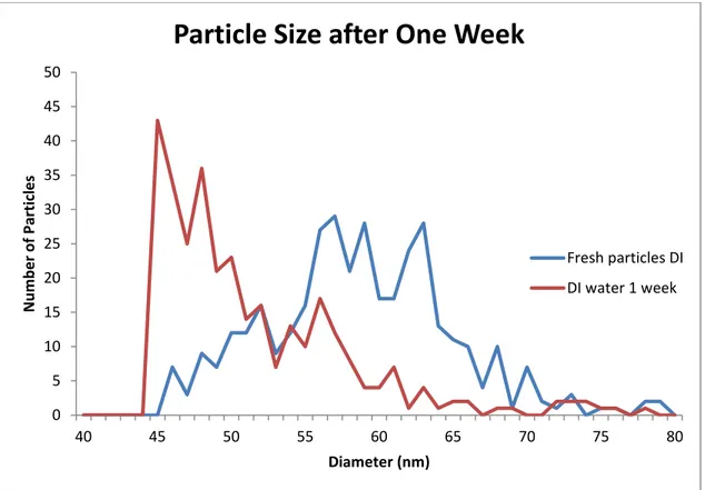
As was previously mentioned the nanoparticles dissolved rather rapidly at low concentration in deionized water. In this experiment the average particle diameter dropped approximately 10 nm in the course of a week (58.8 ± 6.1 for the unaged sample and 49.1 ± 7.5 for the aged samples). This equates to a roughly 32% loss of silver by the particles. The background of the silver was tracked and indicated that the particles were dissolving, not aggregating. This dissolution would release the silver ion into solution which is an environmental issue. The particle size distribution from the experiment can be seen in Figure 2-3.

Figure 2-3: A comparison of fresh and one week old silver nanoparticles. Both started as 60 nm PVP stabilized particles at a 50 ppt concentration.

0 5 10 15 20 25 30 35 40 45 50 40 45 50 55 60 65 70 75 80 N u m b e r o f Par ticl e s Diameter (nm)

Particle Size after One Week

Fresh particles DI DI water 1 week

(30)

18

2.4.2 In natural water

Particle dissolution in natural waters was slower than was observed in the

deionized water. Figure 2-4 shows the distribution of particles from an SP-ICP-MS run. The particles average particle diameter started at 58.8 ± 6.1 nm. Size loss is clearly seen in both though the loss in diameter is far greater in the deionized water sample. The average particle diameter for the filtered lake water sample was 53.1 ± 6.9 nm, the week old DI water sample was 44.6 ± 6.3 nm and the lake water sample had an

average diameter of 49.4 ± 6.5 nm. Particle number loss is also seen though to a lesser extent. Particle loss from the filtered sample was observed to be 2%. Particle number loss form the deionized water was 27% while the unfiltered lake water was 13%. The increase in the background counts indicates that the particles are dissolving not

aggregating. The experiment was initially performed in water from the local Clear Creek but was later performed in water from L239 (the experimental lake in Canada) and filtered water from the lake. The filtered lake water showed the slowest rate of particle dissolution.

2.5 Preservation of particles

The Canadian lake study presented an interesting problem for our lab. The samples needed to be transported from the lake to Canada to the lab in Colorado without the particles being affected in terms of size or number. There were three primary methods that were examined for preserving the particles. The first was a

chemical method of preservation. Nanoparticles are usually coated with a chemical that keeps them in solution. Many different chemical coatings exist but the most widely used

(31)

19

are PVP, citrate, and tannic acid. Simply adding a chemical to the solution to keep the particles in solution would be very advantageous in field work as it is straightforward and easy to accomplish. In order for the samples to be able to be run on the SP-ICP-

Figure 2-4: Particle dissolution in a natural water and DI water.

Data are shown for SP-ICP-MS measurements of 60 nm PVP coated Ag particles made one week after sample preparation. The filtered lake water shows a reduced rate of dissolution compared to the DI and unfiltered lake water which show similar dissolution.

MS we had to ensure that the total dissolved solids did not exceed .01% as the added solids would lead to plasma instability. The second option was a method of freezing. Freezing particles is generally not recommended as it may damage or otherwise change the shape and size of the nanoparticle. Several different types of freezing are available with the two primary methods being flash freezing and standard freezing. Flash freezing is typically done with liquid nitrogen. The freezing process happens so quickly that the water molecules cannot form their typical structure as they solidify. The

0 10 20 30 40 50 60 70 28 33 38 43 48 53 58 63 68 73 N u m b e r o f Par ticl e s Diameter (nm)

Particle Size Change in Natural Water

DI water Lake Water Filtered lake water

(32)

20

main disadvantage of freezing samples is the equipment needed in the field to freeze the samples is quite extensive and can boil off if it is not used in a timely manner. The samples must also be transported frozen which can be problematic for long journeys. Finally oxygen is thought to be the primary reason that nanoparticles dissolve in solution. If the samples have their oxygen removed it is likely that the particles would stay in solution for the trip. This process also has the advantage of easy storage but it would be extremely hard to execute in the field because of the time required and the equipment needed. Ultimately removing the oxygen from the samples was decided to not be an option for preserving the nanoparticles.

2.5.1 Chemical preservation

The chemical preservation experiment looked at three different chemicals, polyvinylpyrrolidone (PVP), mercaptoundecanoic acid (MUA), and citrate. The chemicals would hopefully either prevent oxygen from reaching the surface of the particle and thus prevent particle dissolution, or keep the dissolved silver near the surface greatly slowing the rate of dissolution of the particles. These three chemicals were chosen to avoid overcomplicating the solution. PVP coated particles were to be used in the lake experiment so additional PVP could form an additional protective layer around the nanoparticles. Citrate is another common coating found on particles. It is a smaller molecule and could get bind in areas that PVP could not. Finally MUA was chosen because the sulfide on the end of the molecule will form a strong bond with silver. Additionally the sulfide can be readily oxidized to sulfate using dissolved oxygen.

(33)

21

This process does release hydrogen ions though which may increase the rate of dissolution of the nanoparticles.

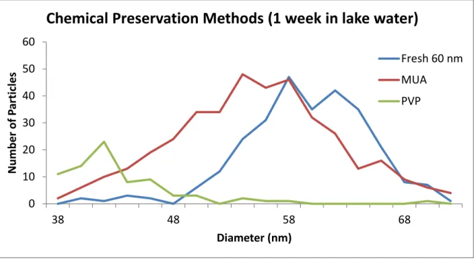
In individual centrifuge tubes particles were diluted to 50 ppt then the chemicals were added. .01% sodium citrate (Sigma S-4641), PVP (Sigma Aldrich PVP40), and mercaptoundecanoic acid (MUA) (Aldrich nanothinks Acid11; 5 mmol in ethanol) were added to their respective tubes. The total amount of Nanothinks added to the MUA samples was .01% of the 5 mmol solution. The tubes were allowed to sit for a week at room temperature in the lab and were then analyzed using the aforementioned method. Figure 2-5 below shows the distribution of the particle diameter after the analysis

compared to a 60 nm PVP particle diluted on the day of the run from the same stock. The particles that were made the day of the run had an average diameter of 58.6 ± 5.1 nm, the samples with the added MUA had an average diameter of 52.3 ± 8.2 nm, and the samples with additional PVP had an average diameter of 45.7. The uncertainty in the mean could not be accurately calculated as the particle distribution was not

completely measurable. The full width at half max for the samples made on the day of the run and the MUA preserved particles are 10 nm and 14 nm respectively.

From figure 2-5 we clearly see the diameter of the particles shrinking with both chemicals added. Citrate was not shown on the graph as the particle diameter and number loss was even greater that that observed in the PVP preserved sample. All of the chemical methods for preserving the nanoparticles did not stop the dissolution process and would not be viable for sending samples back to the lab. The MUA

preserved samples performed the best out of the three possibilities but there was still a loss of approximately 6 nm from the average particle diameter. This equates to a silver

(34)

22

loss of approximately 14%. In order to ensure accurate results the chemical preservation methods will not be useable to ship the samples from the lake to the laboratory for analysis.

Figure 2-5: A comparison of stabilized and fresh nanoparticles.

Preserved particles were analyzed after one week at room temperature using different stabilizers.

2.5.2 Freezing

Freezing particles is not recommended by the manufacturer as it may aggregate or otherwise irreversibly damage the particles [30]. This comes from the manufacturer’s warnings and recommendations that are packed with the particles. The particles that we use come in a concentration of 200 ppm which is rather high. The lake experiment would have a starting concentration of 64 ppb, over three orders of magnitude less than the stock concentration. It was hoped that the concentration would be low enough that

0 10 20 30 40 50 60 38 48 58 68 Nu m b e r of P ar ti cl e s Diameter (nm)

Chemical Preservation Methods (1 week in lake water)

Fresh 60 nm MUA

(35)

23

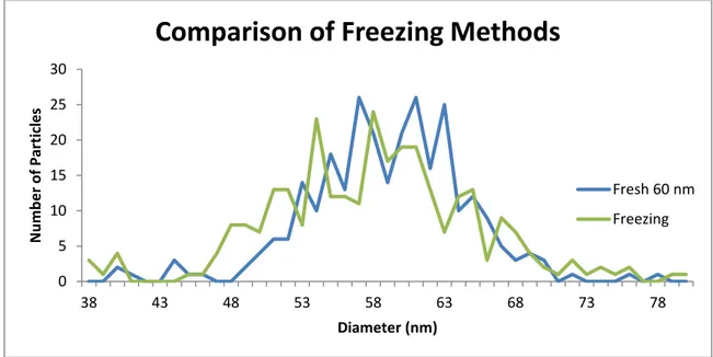
the particles would not aggregate when they were frozen. Freezing would preserve the particles by not allowing oxygen to reach the surface of the particle and would prevent any dissolution of the particle. The freezing would also greatly inhibit any microbial activity that may be present from the samples. The freezer was set to -10 ˚C. The samples were simply placed in the freezer and allowed to freeze. In the field this technique may need some other source of cold in order to freeze the particle as a freezer is impractical in the field. The samples would also have to remain cold for the transportation to Trent University then to CSM. The Figure 2-6 shows the results from the freezing experiment.

The particles lost size when frozen. The loss in diameter was approximately 2 nm. The full width at half max for the sample made the day of analysis was 10 nm while the frozen particles had a full width at half max of 15 nm. No aggregates were

observed in the frozen sample. There were more particles in the 70-80 nm range but no large masses were observed. The lack of aggregates was promising and showed that the freezing method could work with some refinements. The next logical step was to try flash freezing the samples.

2.5.3 Flash Freezing

Flash freezing was the next logical step when freezing the particles was close to preserving the particles. Freezing of any form is not recommended for nanoparticle solutions as listed on the manufacturer’s instructions [30]. The freezing results were promising so flash freezing the samples in liquid nitrogen and storing them in a -80 ˚C freezer until they were ready to be analyzed was tried next. Figure 2-7 shows the results of flash freezing. The particle size distribution stayed the same and the average

(36)

24

also stayed right around the fresh particle diameter. The average particle diameter of the fresh PVP coated particles was 58.3 ± 5.3 nm and the flash frozen particles were-

Figure 2-6: Effect of -10 ˚C freezing on nanoparticle size 60nm PVP capped particles. Particle concentration was 50 ppt.

58.4± 5.2 nm. The full width at half max for both samples was 10 nm. This process was repeated for citrate coated particles where a similar phenomenon was observed. The average diameters were 58.2 ± 6.1 for the sample prepared the day of the run and to 58.0 ± 6.2 nm for frozen particles. The full width at half max was also 10 nm. As liquid nitrogen is hard to handle in the field a dry ice and methanol freezing method was also tried. No difference was observed between the flash freezing and the -80 ˚C freezing was observed. This can be advantageous for collecting samples in the field as it is easier to take dry ice and methanol to the field to work with compared to liquid nitrogen. This was the method that was used to preserve the particles for their trip from the

experimental lake in Canada to the lab at Colorado School of Mines.

0 5 10 15 20 25 30 38 43 48 53 58 63 68 73 78 N u m b e r o f Par ticl e s Diameter (nm)

Comparison of Freezing Methods

Fresh 60 nm Freezing

(37)

25

Figure 2-7: Effect of liquid nitrogen freezing on particle size of 60 nm PVP capped particles. Particles were immediately analyzed (fresh) flash frozen and kept at -80˚C for

(38)

26

CHAPTER 3 :

THE LAKE STUDY

Trent University in Peterborough Canada performed a lake study using the Canadian experimental lakes. Lake 239 was chosen for the experiment. The

experiment would contain two mesocosms into which nanoparticles would be dispersed. The lake would then be monitored for several weeks with data points taken at various intervals. This was a collaborative study involving several universities.

The lake experiment was performed at Lake 239 during the months of July and August 2012. After some discussion it was decided that 50 nm PVP capped particles would be added to the solution so that the particles could still be quantified by the SP-ICP-MS. The mesocosms would be samples for several weeks during the experiment. It was hoped that the fate of silver nanoparticles in the environment could be observed in this experiment.

3.2 Methods

For the lake study experiments 50 nm PVP AgNPs (Nanocomposix, Biopure Formulation silver nanoparticles) were used. The starting concentration was 64 ppm. The particles size was verified using DLS and TEM. The particles were placed into the lake at a 64 ppb concentration. For analysis in the lab, the samples were diluted to a 50 ppt solution by using lake water that had been shipped to us.

(39)

27

. All standards were made the day of the analysis to ensure that the concentration was not effected by other factors.

3.2.1 Collection of Samples

A one-time addition of 50 nm PVP AgNPs (Nanocomposix, Biopure Formulation) was added to two mesocosms to obtain a nominal concentration of 65 ppb based on the theoretical volume of 5340 L. AgNP dosing occurred on July 11th, 2012 with 240 mL of stock solution that was subsequently mixed throughout the water column using a disk. Intensive water sampling occurred the first four days after AgNP dosing to capture the rapid transformations that would initially occur, with subsequent sampling every week. At the center of each mesocosm, the water column was mixed with a disk for a few

(40)

28

minutes before sample collection without disturbing the sediments. Mesocosm water (8 L) was collected from ~10 cm below the surface and pre-filtered through a 35 µm mesh. The collected water was then sub-sampled into 5 mL cryovials, flash frozen, and stored at -80 ˚C until SP-ICP-MS analysis.

3.2.2 Preservation methods

Once the samples were collected they were stored in 5 mL cryovials. The samples were flash frozen in these vials using liquid nitrogen. The samples were shipped in liquid nitrogen to Colorado School of Mines where they were moved to a -80 ˚C freezer where they were stored until the samples were ready to be analyzed. When ready for analysis, the samples were thawed in beaker of warm water. The samples took approximately five minutes to thaw. The samples were then diluted and run on the ICP-MS.

3.3 Results

Samples were analyzed at time points varying from one hour to four weeks. The initial sampling was done at shorter intervals. The concentration of the nanoparticles was too large to be analyzed without dilution on the ICP-MS at CSM. The samples were diluted to 64 ppt for analysis. The unfortunate side effect of this dilution is that it became impossible to track dissolved silver. As dissolved silver ions are the primary reason for silvers toxicity further analysis to obtain this value would be beneficial. A future lake study would be needed to examine any new techniques that may be used to track total silver.

(41)

29

3.3.1 Short term behavior (Less than 1 week)

Short term results were taken from the time points of one week or less. The samples were thawed individually and run immediately after being diluted. The required dilution was 1000 fold. The results showed a Gaussian like distribution with very few coincident readings. The particles started out 49.8 nm which was in good agreement with the data from the manufacturer. By back calculating the dilutions we were able to find he initial silver concentration was 65 ppb which was also in agreement with the target of 64 ppb that the experiment was designed for. Figure 3-1 shows the samples taken from the lake over the course of the first week. The average particle diameter drops from 50 nm one hour after the introduction of the particles to 37 nanometers after a week. This is a very large drop in the particulate silver representing a loss of 63% (from each particle that still exists). The particle diameter may have decreased even more but our lower particle diameter detection limit was 25 nm. The even distribution seen in previous days is truncated at 25 nm in the one week graph. A large decrease in particle number was also observed.

The histograms seen in Figure 3-1 show the number of particles and size distribution. At one week we begin to see the particles run into the background. We also see a longer tail in the data as time progresses. Figure 3-2 shows the decrease in average particle diameter over time. The standard deviation associated with each plug increases over time, a longer tail can be seen in Figure 3-2 as well. This may indicate potential aggregation of some of the particles as they are larger than even the stock particles. Reproducibility between the two plugs was very good and the replicates from each plug also showed very reproducible results.

(42)

30

Figure 3-1: The samples from the first week of the lake experiment showing particle dissolution and loss

(43)

31

As was previously mentioned dissolved silver ions are the primary reason for the toxicity of silver. An attempt to track total silver was made however given the thousand fold dilution needed to analyze the particles in single particle mode it was next to

impossible. Figure 3-3 shows the total silver, particulate silver, and attempt to track dissolved silver. The dissolved silver stays constant indicating that we are simply

seeing noise and we are not able to track the total silver. There are several possibilities for this. First we could have simply diluted the silver background off from the particles. Second is the silver could have bound to some DOC in solution. A different lab involved in the lake experiment used a Field Flow Fractionation (FFF) known as Asymmetric Flow FFF (AF4) and coupled it to ICP-MS. An early eluding silver peak was observed and grew throughout the course of the experiment. The silver could not be dissolved as ionic silver would not make it through the AF4. An ultrafiltration experiment also

showed that dissolved silver did not change over the course of the experiment. This would suggest that we are not diluting the dissolved silver off but the silver is instead bonding with some DOC in solution.

3.3.2 Long term behavior (1-4 weeks)

The longer term lake experiments saw a further degradation of the nanoparticle silver. The particles continued to decrease in size and number. Figure 3-4 shows the average diameter distribution of the particles. The diameter of the particles was small enough that it became impossible to distinguish the particles from the instrumental background. This became impossible at a diameter of 30 nm. For future experiments it may be beneficial to use a shorter dwell time or try SP-ICP-MS fast scan mode in order to distinguish the particles from the background.

(44)

32

Figure 3-3: The mass particulate and dissolved silver over time obtained from integrating the SP-ICP-MS signal.

Figure 3-4: Particle diameter and number over time for long term samples showing dissolution and particle loss.

0 20 40 60 80 100 120 140 160 180 33 39 45 51 57 63 69 75 Par ticl e N u m b e r Diameter (nm)

Long Term Lake Results

1 week lake 2 week lake 3 week lake Initial lake

(45)

33

Figure 3-5 shows the decrease in average particle diameter (blue, left) and particle count (red right) over time. The particle count decreased over nine fold while the average diameter decreased by approximately 15 nm. The average diameter of the silver nanoparticle likely decreased more however the particle diameter distribution began to run into the background and it became impossible to distinguish the two. A more sensitive method on the SP-ICP-MS could be used to analyze the samples and allow for smaller particle sizing and potential of the dissolved silver.

Figure 3-5: The decrease in particle mean diameter and number over time.

0 200 400 600 800 1000 1200 1400 1600 1800 2000 0 10 20 30 40 50 60 0 1 2 3 Par ticl e Co u n t (r e d ) D iam e te r ( n m , b lu e ) Time (weeks)

(46)

34

CHAPTER 4 :

LABORATORY-SIMULATED LAKE CONDITIONS

After the lake experiments took place we attempted to recreate the experiments in the lab using water from the lake. The goal of these experiments was to prepare for a second lake experiment the following summer. The primary goal was to determine what happened to the disappearing particles whether they dissolved, aggregated, or stuck to particles floating in the lake. Ultimately the second lake experiment failed to take place but the research still provided useful insight into the fate of the particles.

The lake experiment was begun in July 2012 and, funding permitting, another would take place in the summer of 2013. In order to collect more useful data the fate of the particles various parameters would have to be examined in the lab so more useful measurements could be taken. It was hoped that dissolved silver could be tracked and a more powerful method for discerning particles from the background could be used.

4.2 Methods

For the laboratory recreation experiments 60 nm PVP capped NanoXact silver nanoparticles from Nanocomposix (San Diego, CA) were used. The starting

(47)

35

particle diameter was found to be 55 ± 5.3 nm. The particles were diluted to the appropriate concentration using the proper corresponding water.

. All standards were made the day of the analysis to ensure that the concentration was not effected by other factors.

4.3 Matrices

The first factor that was examined was the effect of the matrix on particle

diameter and number. The lake water had relatively high amounts of dissolved organic carbon which could go a long way in stabilizing nanoparticles [31]. The effects of DOC on silver ions are not as well understood. If we wish to track total dissolved silver it is important to understand how silver ions are affected by differing matrices. For analysis

(48)

36

the calibration slope for silver is always found in a 2% nitric acid matrix. The first step in this experiment was to determine if the matrix had any major effect on the detection of silver. Differing dissolved silver standards were diluted to 500 ppt in various matrices and analyzed. Figure 4-1 shows the difference between the normal analysis (2% nitric acid), 10% nitric acid, and lake water. These samples were diluted and run the day of analysis. We see that the higher acid concentrations led to more silver counts in the dissolved standards while the lake water had fewer counts. Acid is typically used to prevent silver from falling out of solution or from adhering to the sides of the tubes. This observation was what was expected. In the event that SP-ICP-MS is used to track the dissolved silver in the lake it will likely read less dissolved silver than there is actually in solution. It is possible that silver stuck to the sides of the tubes during analysis but a loss in silver would still need to be accounted for in any future experiments.

Next sample calibration curves were made in DI water, 10% nitric acid, 2% nitric acid, and lake water. The samples were run twice, once just after being freshly

prepared, and again three days later so a change could be observed. Figure 4-2 shows the fresh calibration curve. The 10% acid curve is the steepest as was expected from the previous results, followed by the 2% acid, then the deionized water and finally the lake water. The steepness corresponds directly to the sensitivity of the instrument meaning that the instrument is more sensitive to solutions in 10% nitric acid. The slope could have to do with different nebulization efficiencies which would indicate that

something in the lake water is binding with the dissolved silver and reducing its chance of entering the spray chamber with the rest of the dissolved silver.

(49)

37

Figure 4-1: The % change in 107Ag counts for a 500 ppt dissolved silver diluted in lake water and 10% nitric acid as compared to 2% nitric acid..

Figure 4-2: The calibration slopes for dissolved silver in lake water, DI water, 2% nitric acid and 10% nitric acid immediately after preparation.

-15 -10 -5 0 5 10 15 20 25 % c h an ge r e lativ e to 2% HNO3

Percent Change in Counts Relative to 2% acid

500 ppt 10% 500 ppt lake 0 50 100 150 200 250 300 350 400 450 500 0 100 200 300 400 500 600 Co u n ts Concentration (ppt)

Concentration vs. Counts (fresh)

2% f 10%f DI F LW F Linear (2% f) Linear (10%f) Linear (DI F) Linear (LW F)

(50)

38

After three days the samples were rerun and the slopes of the calibration curves were analyzed again. The order of steepness between the different waters was again observed. The details can be seen in Figure 4-3. A decrease in all the slopes was also observed. Given the history of silver adhering to the sides of tubes this is not surprising. The lack of loss of the dissolved silver from the deionized water sample did come as a surprise as there is no acid to keep the silver in solution or hydrogen to adhere to the plastic tubes to prevent silver adsorption.

Figure 4-3: The calibration slopes for dissolved silver in lake water, DI water, 2% nitric acid and 10% nitric acid prepared three days prior to analysis.

The negative percent change in the silver concentration over time is shown in Figure 4-4. This silver decrease in the lake water over the course of three days was quite drastic, approximately 27%. If samples are to be transported this is very important as a large loss in silver could greatly affect the results. Different natural waters could be

0 50 100 150 200 250 300 350 400 450 500 0 100 200 300 400 500 600 Co u n ts Concentrtaion (ppt)

Concentration vs. Counts (3 day)

2% 10% DI LW Linear (2%) Linear (10%) Linear (DI) Linear (LW)

(51)

39

affected differently as well. In the future, when tracking total dissolved silver, using a scaling factor will be important to track the total dissolved silver.

Figure 4-4: The percent change in counts over three days of dissolved silver standards relative to their respective matricies.

4.4 Tracking total silver

The total silver could not be tracked in the lake samples, possibly because of the large dilution of the background silver. The fate of these nanoparticles in the

environment is very important as dissolved silver ions will behave differently than silver nanoparticles which will behave differently from aggregated silver. Silver aggregating would be the best way for silver to be removed from a natural water system. In an attempt to track total silver an experiment was designed which would allow us to perform this. 60 nm PVP capped nanoparticles were diluted to 50 ppt in deionized

0 5 10 15 20 25 30 35 2% 10% DI LW Ch an ge ( -%)

(52)

40

water and allowed to sit for a week. After a week the samples were run using the above mentioned method. The remaining sample was then disposed of and 10 ml of new DI water was added to the samples. The samples were then sonicated for a minute, and then run again. This was repeated once more. The tubes were then soaked in a 5% nitric acid solution, sonicated, and run again to remove any lingering particles or silver that may adsorbed to the tube. This was repeated three times and the total silver was summed in an attempt to obtain the total silver in solution. In order to obtain the total silver in solution the mass of silver in particle form was divided by the nebulization efficiency, the background from the samples was then added after subtracting the instrumental background. This was done for each particle sample. The acid rinses were added to the total after the instrumental background was subtracted off. The particles had shrunk over the course of a week to an average of just over 50 nm. This would lead to an increase in dissolved silver background. The smallest particle

diameter that could be detected was 29 nm so any particles that were smaller than that would be in the background and could lead to potential errors in the silver tracking. Figure 4-5 shows the average diameter of the particles from the initial run and the first sonication rinse afterward. The first run was the only one that had any appreciable amount of particles in it. Relative to the initial run the first sonication had 17% of the particle number and an additional loss of approximately 3 nm in diameter. There was a much larger tail in the sonicated samples than there was in the initial run though the bulk of the particles were smaller in the sonication run.

The math for tracking the total silver was as follows. The dissolved background was converted to mass using the mass calibration slope from the beginning of each run.

(53)

41

This represented the mass of dissolved silver detected in the solution. The mass of particle silver was found and divided by the nebulization coefficient to give the total mass of silver that was in particle form. Only a small percent of the silver nanoparticles actually make it through the nebulization process and through the cones into the spray chamber thus in order to find the total mass of particulate silver it is necessary to divide by the nebulization coefficient. The mass of the dissolved standard already takes this into account

Figure 4-5: Comparison of initial of 60 nm PVP capped Ag to particles recovered from container by sonication.

The nitric acid rinses removed an appreciable amount of the silver that was still in the centrifuge tubes. Figure 4-6 shows the sequential rinses in terms of raw counts. By comparison a blank will measure between 8000-12000 counts typically. This is still elevated and the last rinse still had several ppt silver present in it. Whether this silver

0 5 10 15 20 25 25 30 35 40 45 50 55 60 65 70 75 80 N u m b e r o f Par ticl e s Diameter (nm)

Silver Recovery

Low B (sonic initial) Sonicated B

(54)

42

adsorbed to the side of the centrifuge tubes, came off from the pump tubing during analysis, or came from elsewhere could not be accurately determined. When the particulate silver was added with the background, and the acid rinses on average only 85% of silver could be accounted for. This is substantially less than the amount that was in the sample. Several possibilities exist for the location of the silver. It could still be adsorbed to the instrument tubing, or it could be adsorbed to the centrifuge tube. Finally it could have aggregated and fallen out of solution and been disposed of with the rest of the waste. It is not possible to determine which one is true from the available data. By using the previously mentioned calculations it is also possible that some of the silver particles were detected in the background and were therefore not divided by the nebulization efficiency and thus silver was lost in the calculations. A future experiment using an acid digestion to completely digest the particles could be used as a base in order to obtain an accurate baseline silver concentration in the solution. A particle size separation method in addition to the SP-ICP-MS could be used to determine the fate of the silver though higher concentrations would be required. Table 4-1 shows the results of the silver tracking experiment for a set of three samples. The total silver that was recovered after a week was typically around 85%, consistently below what is recovered for a sample that was prepared immediately before the run, even with the additional rinses added to the total. The large amount of tubing connecting the autosampler to the ICP-MS may be a location where some of the silver particles or dissolved silver

adsorbed. An acid rinse occurs between every sample and this silver is likely lost for good using this analysis technique. The amount lost to this should be very small though.

(55)

43

Figure 4-6: The measured counts for silver removed by subsequent acid rinses of the container.

Table 4-1: The results from the laboratory silver tracking

4.5 Effect of water composition on short-term stability

As has previously been established DOC and various other types of water parameters can play a large role on the stability of nanoparticles [32]. Silver

nanoparticles seem to degrade far more quickly in DI water than in natural waters. The reason for this is not fully understood. In an attempt to understand why the particles

0 20000 40000 60000 80000 100000 120000 140000 160000 180000 200000

Low Acid Rinse A Low Acid Rinse B Low Acid Rinse C

Co

u

n

ts

Sequential Acid Rinse Silver

Name Particle Mass (initial) Diss. mass (initial) Rinse (particle) Rinse (diss) Acid Rinse 1 Acid Rinse 2 Acid Rinse 3 Total % recovery 50 ppt Diss. 0 9.35E-06 0 0 0 0 0 9.4E-06 100.00 Particle new 8.33E-06 7.57E-07 0 0 0 0 0 9.1E-06 97.19 1 week A 4.49E-06 1.27E-06 6.74E-07 7.50E-07 2.34E-07 1.87E-07 1.59E-07 7.8E-06 83.13 1 week B 4.58E-06 1.31E-06 7.46E-07 8.11E-07 2.22E-07 1.73E-07 1.51E-07 8E-06 85.43 1 week C 4.21E-06 1.32E-06 5.89E-07 7.89E-07 2.41E-07 1.91E-07 1.44E-07 7.5E-06 79.98