Abstract—The use of systems analysis involving tools like Causal loop diagrams and stock and flow diagrams can be shown in practical tests to greatly enhance systems insight and understanding of the dynamic behaviour of complex systems. Whereas many students may have difficulty understanding what a coupled system of differential equations really do, systems analysis creates such insights even to those with differentiofobia. Within the systems analysis course given at LUMES, we have extensive experience in teaching systems analysis and the use of CLD and SFDs to people of different backgrounds, and also seen how technical problems in engineering have a great help in using CLD and SFDs to explain and communicate insight into complex systems to non-technical people
Index Terms—systems thinking, systems analysis, complex systems
I. INTRODUCTION
O be an engineer is to be able to understand dynamic systems sufficiently that one can design e.g. large bridges, biochemical reactors, wireless Internet protocols, etc. However to reach the necessary ‘eagles perspective’ is a daunting task. One of the great risks in engineering education is that the students may fail to reach this perspective and instead focus on mathematical recipes and details of different systems without ever acquiring the ability to put it all together. The engineering analytical process always begins with a conceptual model where thinking is translated from an idea onto a paper. This has traditionally been portrayed through the ‘stock and flow’ diagram (SFD) concept which has its tradition back to the 1920’s (1). Stock and flow diagrams have been used for understanding processes as aiding tools for deriving differential equations. They are used to understand the flow and fluxes of quantities but lack the ability to illustrate the information associated to the flow and fluxes.
Communicating the understanding of SFD and systems of
Manuskript mottaget 18 april 2006.
H. Haraldsson är forskarassistent vid institutionen för Kemiteknik, Lunds Universitet, Box 124, 221 00 Lund (Hordur.Haraldsson@chemeng.lth.se)
H. Sverdrup är professor vid institutionen för Kemiteknik, Lunds Universitet, Box 124, 221 00 Lund (harald.sverdrup@chemeng.lth.se)
S. Belyazid är doktor vid institutionen för Kemiteknik, Lunds Universitet, Box 124, 221 00 Lund (salim.belyazid@chemeng.lth.se)
differential equations can only be done if the students speak the same language using the same terminology and expressions for describing the systems. In engineering it is apparent that communicating the results is as important as generating them. Forrester (2) therefore developed the Causal Loop Diagram (CLD) concept as a part of communicating complex SFD system into simplified feedback structure. The CLD was initially regarded as a posterior tool for describing a ‘ready made’ simulation but it was soon discovered that a CLD could be used as an aid for conceptualizing a hypothesis for a problem (2) .
The Causal Loop Diagram is a tool for systematically identifying, analysing and communicating feed back loop structures (3). It is a systematic thinking and enables communication of complex information into simplified circular loop feedback structure. CLD's is a tool that promotes 'continuous' thinking, i.e. a story of a problem is read through the diagram and its development projected on a 'time scale graph' in order to understand the interaction of the feedback loop structure in the diagram. In the engineering education this has proven to be an excellent supplement towards better understanding the information associated to the 'stock and flow' structures in relation to their related information and feedbacks.
Together, the Stock-and-flow diagram and the Causal Loop diagram fully defines the differential equation system, however, the representation is much easier to communicate and understand in terms of feedback structures and basic dynamic behaviour of the system. This allows for the student a system insight normally denied by observing the equation system alone in its traditional mathematical notation. However, this notation is easily derived from the diagrams. II. EXPLAINING THE CAUSAL-LOOP-DIAGRAM (CLD)
The CLD help us to create a systematic understanding how changes manifest in the problem. Cause and effect variables either change in the same direction (indicated with a “plus”) or change in opposite direction (indicated with a “minus”). Processes that feedback in the same direction are called reinforced processes (indicated with R) since they amplify the condition. Similarly, the processes that feedback to give a
Causal Loop Diagrams–promoting deep
learning of complex systems in engineering
education
Hördur V. Haraldsson, Salim Belyazid, Harald U. Sverdrup
change in opposite direction (indicated with B) balance (dampen) out a condition (figure 1).
P opulation
R B D eaths
B irths
Figure 1: Population increase is reinforced by number of births whereas the number of deaths reduces the population and dampens the effect of the reinforcing loop.
III. EXPLAINING THE STOCK-AND-FLOW DIAGRAM (SFD) Stock and Flow diagrams are used to show flow dependencies and how quantities are distributed within a system. Stocks hold quantities that are either subject to accumulation, through inflows or subject to reduction through outflows (figure 2).
B irths P opulation D eaths
Figure 2: Population is indicated as stock since the number of people constitutes as quantity. The numbers of people being born are flowed as new individuals into the population, whereas as the number of people dying flow individuals out from the population.
IV. FROM CLD AND SFD TO DIFFERENTIAL EQUATIONS
The combination of the CLD and SFD allows us to create differential equations structure that can be checked against the conceptual models. In system dynamic education and research, system dynamic-tools (SD-tools) are used to run the numerical simulations. These SD-tools use System Dynamic Tool Diagrams (SDTD) that is graphical versions of the mental model, adapted for the numerical domain from the CLD and the SFD. The SDTD is a hybrid of SFD and CLD and used in SD-tools to numerically simulate models (4). The process of building a numerical model rests on a mental model, mapped through CLDs and SFDs. Using an SDTD as a continuation to the qualitative stage not only illustrates the feedback processes and causalities but simultaneously the properties of the variables in the model (i.e. a stock or flow).
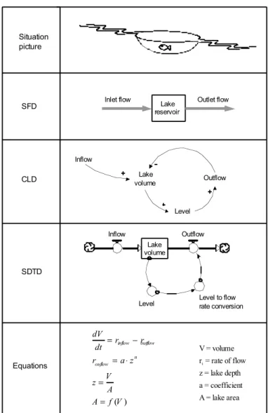
For each problem solving there are five stages in the analysis phase (4, 5); 1) The situation picture illustrating the system state, 2) SFD for identifying pathways and quantities. 3) CLD for identifying the feedback loop structure 4) Merging of the SFD and CLD into SDTD for generating 5) the differential equations (figure, 3).
Inflow Lake volume Level Outflow Lake volume Inflow Outflow
Level Level to flowrate conversion Lake
reservoir
Inlet flow Outlet flow
Situation picture SFD CLD SDTD Equations ( ) inflow outflow n ouflow dV r r dt r a z V z A A f V = ! = " = = i V = volume r = rate of flow z = lake depth a = coefficient A = lake area
Figure 3: The five analysis phases.
Below is a simple demonstration of how the use of a CLD and a SFD is used to derive differential equations and produce a problem solving strategy. The learning goal for the student is to understand how a simple stirred tank reactor works by illustration it through a salt mixing with water. There are several answer possible depending on the detailness of the answer.
A farmer called John has just installed a new water tank that is intended for drinking water. He has constructed a tank with 1000L capacity and attached a tube from the local water spring which has an inflow of 5L/min to the tank. Similarly he has attached an outflow tube in order to maintain a constant volume in the tank. After John had installed the in and out flow tubes and filled up the water to its max capacity he had a small accident. One of his packets of salt that was stored on the shelf above the tank was accidentally knocked over and fell directly into the water. The salt dissolved directly. John decided to estimate how long it would take for the salt to be out of the tank.
create a salt concentration. Furthermore, illustrate how the salt leaves the system.
Questions: 1) How is the salt concentration in the water reduced? 2) How many minutes are needed to reduce the salt concentration by 75%?
In order to answer question 1, the first task is to create the CLD that shows how the salt concentration is dynamically linked in a CLD and SFD for showing flow pathways as well as quantity (figure 4-5).
Water in
Salt in Salt in water
Concentration
Water vol Water out
Salt out + -+ -+ + + +
-Figure 4: The CLD of the salt being mixed into the water.
water in Salt in W ater vol water out Salt in water Salt out
Figure 5: The SFD of the water and salt is created as well as their flow pathways.
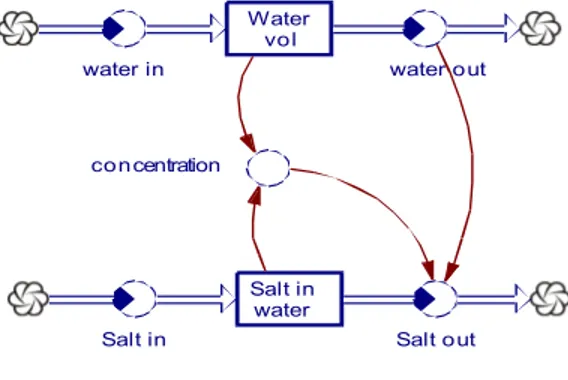
In order to answer question 2, the SFD is created and combined into a SDTD (figure 6).
water in concentration Salt in Water vol water out Salt in water Salt out
Figure 6: The combined CLD and SFD allows for us to realise the differential equation structure.
If a simple conceptual illustration is only required then CLD and SFD may fulfil that answer. If the answer requires a numerical accuracy then the problem can be investigated further with a SDTD and modelled in a SD simulation software.
By looking at the diagrams, we can now see how the differential equations must look for the mass balance for salt in the water tank (figure 7). We know that the salt flow out (Mout) must be the water flow (Qout) times the concentration in
the out stream (C):
*
out out
M
=
C Q
and according to the principle of a stirred tank, then the concentration (C) is equal to:
M
C
V
=
And the amount of salt (Msalt) in the tank is the concentration
(C) times that volume (V):
*
saltM
=
C V
Qin V Qo u t Min M Mo u t C M V =Figure 7. The equation system laid out into the CLD diagram. From this we may construct the equation system in standard notation.
We can then put together the differential equations that exactly corresponds to our CLD and SFD:
in out
dV
Q
Q
in out
dM
M
M
dt
=
!
and for the concentration:
(
in*
in out*
)
/
dc
Q
C
Q
C V
dt
=
!
(
)
(
)
(
)
21
*
in out*
in out*
dC
V
M
M
M
Q
Q
dt
V
!
"
=
$
#
#
#
%
&
'
The diagram shows very clearly how the water dynamics affect the concentration, and how the concentration in turn determines the amount that leaves the tank with the outflow. The student can now first understand the principles, and then create the proper equations by using his graphical representation of the system.
V. GROUP MEDIATED MODELLING AND COMMUNICATION
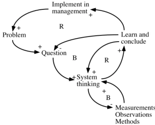
Randers (2), makes a clear distinction between the qualitative ‘conceptual phase’ and the quantitative ‘equation phase’ of the procedure. The ability to ask the right questions depends on the ability to put together a group of people with the sufficient background knowledge in order to get as correct definitions to the problem as possible. The CLD reflects the understanding of the problem, therefore the problem definition and the questions asked concerning the problem are reflected in the CLD. This process is done through group model building, as advocated in Vennix (6, 7). When a group of people are faced with a specific issue, mental models are depicted differently in each person observing the problem. Miscommunication may exist within the group due to differences of the mental models when they are put to the test against each other. Group model building uses a process to bring together different mental models to find the common denominator that can help the group members to discover each others mental models (8). Group model building strives to create a shared mental model for the group. This process starts by framing a question for the problem (figure 8). The question takes the form of a hypothesis for the group to work by, where it is either verified or refuted through several iterations as a continuous learning process called the ‘Learning Loop’ (4, 9).
Problem Question System thinking Measurements Observations Methods Learn and conclude -+ + + -+ B R B Implement in management + + R +
Figure 8. The learning loop is the basic scientific behavior trained with the student for any type of problem-oriented work.
VI. THE PEDAGOGICAL ADVANTAGES OF SYSTEMS ANALYSIS TOOLS
The learning loop is continuously drilled into the students as the basic scientific behavior to be adopted for problem based work. With system thinking we imply the constructions of models as a means to learn how to solve the problem, by investigation, taking apart and reassemble the insights to reconstruct the system through a model that allow for recreation, prediction and subsequently design. And as we know, engineering is all about design and predictability. In Figure 9, we may develop further into the full flowchart for how to work. Start SDTD SBIC CLD SFD SD-predictor Numerical Domain Machine code Fortran, C++, Java, etc
Equation system
Qualitative simulation
Back of the envelope-qualitative simulation Systemic simulation Mathematical modelling Numerical simulation using high performance methods Definition Clarification Confirmation Implementation
Figure 9. The workflow moves through four phases, where it is necessary to be aware of where the student is in the flow (5).
VII. CONCLUSIONS
The methodology outlined here gives the student a logical procedure for how to build his understanding of a system, an
priority over by-heart learning of formula. Then the student can always reconstruct what is needed from his understanding and a consistent process. Our experience is that students using this method goes through a number of revelation experiences with traditional chemical mechanisms and processes when they suddenly realize what really goes on The work approach greatly enhances the communication of the results afterwards, as well as it transforms what many chemical engineering students learn as an acquired handcraft into a conscious science (10). Knowing what you are doing is good, understanding what you do is superior.
VIII. REFERENCES
[1] 1. W. H. Walker, W. K. Lewis, W. H. McAdams, Principles of
Chemical Engineering (McGraw-Hill, 1923), pp. 450.
[2] 2. J. Randers, Elements of the System Dynamic Method (Productivity Press, Cambridge, 1980), pp. 320.
[3] 3. G. P. Richardson, System Dynamics Review 2, 158 (1986). [4] 4. H. V. Haraldsson, PhD, Lund University (2005). [5] 5. H. V. Haraldsson, H. Sverdrup, System Dynamics Review
submitted (2005).
[6] 6. J. A. M. Vennix, System Dynamics Review 15, 379 (1999). [7] 7. J. A. M. Vennix, Group Model Building (Wiley, New York, 1996),
pp. 297.
[8] 8. J. A. M. Vennix, H. A. Akkermans, A. J. A. Rouwette, System
Dynamics Review 12, 39 (1996).
[9] 9. H. V. Haraldsson, H. U. Sverdrup, in Environmental Modelling:
Finding Simplicity in Complexity J. Wainwright, M. Mulligan, Eds.
(Wiley, New York, 2004) pp. 211-223.
[10] 10. P. Wallman, M. Svensson, H. Sverdrup, S. Belyazid, Forest