http://www.diva-portal.org
Postprint
This is the accepted version of a paper published in IET Intelligent Transport Systems. This paper has been peer-reviewed but does not include the final publisher proof-corrections or journal pagination.
Citation for the original published paper (version of record):
Silveira, C S., Cardoso, J S., Lourenco, A L., Ahlström, C. (2019)
Importance of subject-dependent classification and imbalanced distributions in driver sleepiness detection in realistic conditions
IET Intelligent Transport Systems, 13(2): 347-355
https://doi.org/10.1049/iet-its.2018.5284
Access to the published version may require subscription. N.B. When citing this work, cite the original published paper.
Permanent link to this version:
1 The importance of subject-dependent classification and imbalanced distributions in driver sleepiness detection in realistic conditions
Cláudia Sofia Silveira 1, Jaime S. Cardoso 1, 2*, André L. Lourenço 3, Christer Ahlstrom 4
1 Faculty of Engineering of University of Porto, Portugal 2 INESC TEC, Porto, Portugal
3 CardioID Technologies Lda., Porto, Portugal; High Institute of Engineering of Lisbon, Portugal
4 The Swedish National Road and Transport Research Institute (VTI), Linköping, Sweden; Department of
Biomedical Engineering, Linköping University, Linköping, Sweden
*jaime.cardoso@inesctec.pt
Abstract: The first in-depth study on the use of electrocardiogram (ECG) and electrooculogram (EOG) for subject-dependent classification in driver sleepiness/fatigue under realistic driving conditions is presented in this work.
Since acquisitions in simulated environments may be misleading for sleepiness assessment, performing studies on road are required. For that purpose, we present a database resulting from a field driving study performed in the SleepEye project. Based on previous research, supervised machine learning methods are implemented and applied to 16 heart- and 25 eye-based extracted features, mostly related to heart rate variability and blink events, respectively, in order to study the influence of subject dependency in sleepiness classification, using different classifiers and dealing with imbalanced class distributions. Results showed a significantly worse performance in subject-independent classification: a decrease of approximately 40% and 20% in the detection rate of the “sleepy” class for two and three classes, respectively. Since physiological signals are the ones that present the most individual characteristics, a subject-independent classification can be even harder to perform. Transfer learning techniques and methods for imbalanced distributions are promising approaches and need further investigation.
1. Introduction
Every year, approximately 1.25 million people die on road worldwide [1]. Regarding all driving accidents, it has been estimated that sleepy/fatigue driving is the cause of more than 100,000 crashes each year (up to 20% of all accidents), including 76,000 injuries, 1,500 deaths and 12.5 billion dollars loss [2, 3]. Unfortunately, despite existing countermeasures, such as promoting adequate sleep, and although the total number of fatalities has been decreasing gradually, the percentage due to sleepy driving has been consistent [4].
In order to minimize injuries and prevent accidents, intelligent sleepiness monitoring systems have been introduced as a way of providing safety to drivers and some systems are already available in the market. These systems are mostly based on vehicle-based measures, but they are dependent on several external factors, such as road conditions and, therefore, they are not reliable [5]. Physiological signals are the most promising measures for designing a robust model for fatigue detection, since they measure the driver directly. Driver sleepiness detection using physiological signals can combine several sensors to measure different signals, such as electrocardiogram (ECG), electromyogram (EMG), electrooculogram (EOG) and electroencephalogram (EEG), creating a more complete but also more complex system.
From a driving research perspective, performing tests with vehicles in real traffic is the ultimate validation step. In order to carry out experiments, most researchers have used simulated environments for sleepiness manipulation due to the fact that it is not safe to perform tests on real roads [6, 7, 8, 9, 10, 11, 12]. However, simulated data, resulting from the acquisition in driver simulator environments, may be misleading for fatigue assessment. The acquisition of data from simulated environments and on road can result not only in different reactions from the drivers but also in different classifications and perceptions of drowsiness. Recent studies have revealed that simulators can cause higher sleepiness levels than real driving, since drivers become more aware of external and environmental factors that can affect their performance [13, 14]. Additionally, drivers are more careful and control much better the vehicle (lane deviations, for example), in real driving.
2 In this work, we present the first in-depth study on the use of only ECG and EOG for subject-dependent fatigue classification under realistic driving conditions. Over this database, we perform a detailed comparative study of different methodologies for sleepiness detection. Supervised machine learning methods are implemented in order to investigate relatively unexplored aspects regarding driver’s state monitoring on road, focusing on subject dependency and imbalanced class distributions. The remaining of the paper is organized as follows. Section 2 covers the main information about prior art in the area of fatigue detection, with focus on physiological signals and their relation to sleepiness and fatigue, as well as information about existing databases in realistic conditions. Regarding ECG and EOG, we present an overview of the most important features. Section 3 presents the database used in this work, acquired under realistic conditions. Section 4 deals with the preprocessing of ECG and EOG signals and the detection of eye and heart movements. Afterwards, extracted features are introduced, mostly related to features extracted from blinks and from heart rate variability (HRV) signals. Finally, Section 5 presents the results of sleepiness classification based on extracted features, mentioned in the previous section, using machine learning methods.
2. Related Work
Previous studies cannot be fairly compared, since they are different in several aspects, such as sources of information (non-physiological and multiple physiological measures, for example ECG, EEG, EOG and EMG + EEG), experimental environment (simulated or road), number of subjects, obtained labels and metrics for performance evaluation.
Since it is quite difficult and challenging to define and evaluate fatigue levels, just a few databases are reported in the literature for this application, such as RDB (Real Driving Database), a private database used in several studies and provided by Fico Mirrors S.A. company [10], [15], [16], [17]. RDB consists of ten recordings of ten professional drivers (eight male and two female) that were not sleep-deprived. Driving sessions were performed during eight hours in highway and city roads (with breaks of ten minutes every two hours). A 2-lead ECG signal, EEG signals and video recordings were measured and external observer annotations were also made. Since this database is private, most of researchers have focused on their own acquisitions. In the study presented by Rigas et al. [18], experiments were performed on road using physiological signals (ECG, electrodermal activity and respiration) and also video recordings from the driver’s face and environmental information. However, only one subject participated in the experiments, limiting the relevance of the study. These studies have focused on ECG signals, proving that it is possible to associate ECG features with drowsiness, adding improvements to existing car safety systems. In another study presented by Mårtensson et al. [19], a larger real road database containing ECG, EOG, EEG and driving performance measures was used, showing that there is a need for more research on how subject dependency influence driver sleepiness detection.
Regarding the ECG signal, the most commonly extracted features are related to heart rate variability (HRV), since heart rate becomes more irregular as the driver gets sleepy [6], [10], [15], [16], [17], [18], [20], [21], [22], [23], [24], [25], [26]. HRV measures beat-to-beat changes in the heart rate, describing instantaneous variations on RR intervals, also called normal-to-normal (NN) intervals [27]. The HRV signal can be obtained through R peak detection algorithms. In order to extract HRV features, frequency or time methods can be followed. Frequency domain methods are based on power spectral density (PSD) analysis. This analysis provides basic information about power (variance) distribution as a function of frequency [27]. Fast Fourier Transform (FFT) is the simplest, fastest, more accurate and most well-known method for computing PSD. Parameters such as power in the VLF (very low frequency) band (0.003 to 0.04 Hz), in the LF (low-frequency) band (0.04 to 0.15 Hz) and in the HF (high-frequency) band (0.15 to 0.4 Hz) and even the ratio LF/HF can be extracted. Some researchers considered that LF and HF are reliable measures of sympathetic and parasympathetic activity, respectively, and the ratio LF/HF describes the balance between those activities [10], [15], [24], [28], [29]. Since wakefulness states are related to an increase of sympathetic activity and relaxation states are dominated by a parasympathetic activity, a transition from wake to sleep can be noticed as an increase of HF power or a decrease in LF, and consequently as a decrease in LF/HF ratio [6], [15], [17], [29], [30]. In contrast, awake states have been associated with higher LF/HF
3 [10]. Regarding time domain methods, statistical features are commonly used [10], [22], such as SDNN (standard deviation of NN intervals) and SDSD (standard deviation of differences between adjacent NN intervals) [27].
Regarding the EOG signal, it is possible to detect eye blinks from the vertical channel, saccades or fast eye movements from the vertical and horizontal channels and also slower movements, mostly from the horizontal channel. These types of movements are distinguishable using peak detection techniques and velocity analysis, including thresholding and first order derivative methods [31], [32], [33], [34], [35], respectively. Based on blinks and saccades, several features can be extracted and are related to frequency, duration and velocity [31], [36], [37]. In most cases, and as already said, rapid eye movements (shorter blinking durations and shorter pauses) are related to awake states and slower ones (longer blinking durations, higher closing times and longer pauses) are related to sleepiness states [36], [38]. Recently, these ocular movements, in particular eye blink parameters, have been used to study driving events in shift workers for indicating drowsiness levels [39],[40].
3. Material and Methods
A total of 20 participants (10 women) were recruited from the Swedish National Register of vehicle owners. Inclusion criteria were: between 30 and 60 years old, good self-reported health, normal weight, and no shift workers or professional drivers. Approximately two weeks before the experiment the participants received detailed information about the upcoming experiment together with sleep and wake diaries that were to be filled in the three nights and two days prior to the experimental day. They also received background questionnaires. In addition, the scale to use for reporting self-reported sleepiness (Karolinska Sleepiness Scale, KSS) was sent home together with instructions and a training program to learn how to rate KSS. Permission to conduct driving sessions with sleep deprived drivers on public roads was given by the Swedish government (N2007/5326/TR). The study was approved by the regional ethics committee in Linköping (dnr 2010/153–3).
The participants prepared for the experiment by sleeping for at least seven hours the three nights prior to the test. On the experimental day they were instructed to get up no later than 7:00 a.m. The participants were also requested to avoid alcohol for 72 h and to abstain from nicotine and caffeine for 3h before the first driving session until the end of the experimental day. Each driver performed one driving session during daytime (supposedly alert condition) and one session during night-time (sleep deprived condition). Two participants took part in the experiment on the experimental day. The first participant of the day started to drive at 15:30 (alert condition) and at 00:15 (sleep deprived condition), while the second participant of the day started to drive at 17:45 and 02:45, respectively. The driving session lasted for about 90 minutes and was conducted on a motorway on the public road E4 outside the city of Linköping, Sweden. The posted speed limit was 110 km/h and the annual average daily traffic for this road is 9000 - 14000 vehicles. The car used in the experiment was a Volvo XC70 with an automatic gearbox. A test leader accompanied all participants and was seated in the front passenger seat. The car had dual command and the test leader was prepared to take control of the vehicle if the driver became too sleepy.
Different ground truths of driver sleepiness have been used for sleepiness classification, including expert ratings based on video recordings [28], [41], expert ratings based on physiological signals [42], the supposed alertness level that follows from an experimental design with sleep deprived participants [43], the percentage of eye closure [44], and lane departure events. However, video based expert ratings have been found to be unreliable [45], the experimental design approach does not guarantee that the driver is alert in the supposedly alert condition, and lane departure events are rare in themselves and only reflect the rather rare lapses in attention that follows from sleep deprivation (so called wake state instability) [46]. All in all, subjective ratings seem to be the better alternative, especially since KSS is easily applied and unobtrusive. The participants were asked to evaluate their state using the KSS scale (9 levels: 1 (extremely alert); 3 (alert); 5 (neither alert nor sleepy); 7 (Sleepy, but no effort to keep alert; 9 (Very sleepy, great effort to keep alert, fighting sleep) [47]) at 5-minute intervals and physiological data were recorded by a Vitaport 3 (TEMEC Instrument BV, Kerkrade, the Netherlands). More details can be found in [48]. There are cases
4 of really alert and also very sleepy states, covering almost the full range of KSS ratings for each participant (see Fig. 1.).
4. ECG and EOG-feature-based methodology for monitoring driver’s state
In this section, we detail the adopted methodology. We employ a preprocessing specific to each modality, followed by an also modality-specific feature extraction. Instead of limiting any subsequent analysis to an initial choice of a (few) feature(s), and since previous guidelines on simulated environments may not hold on a realistic setting, we decided on extracting a wide range of well-known features - and some new ones introduced in this work - with the purpose of proceeding later to a feature selection analysis.
4.1.
Preprocessing and feature extraction
4.1.1 Electrocardiogram
Preprocessing consisted in a bandpass Butterworth filter with cut-off frequencies of 4 Hz and 50 Hz. The combination of a low-pass and a high-pass filter eliminates high frequency noise, especially related to power line interferences (50 Hz) and electromyogram induced noises, and baseline wander due to respiration or motions, respectively.
For R peak detection, the signal was divided into two-minute windows. On each window, 0.75-second windows were selected with no overlap and for each one, the local mean of the signal was computed. While the signal is above the local mean, the corresponding region is being selected. When the signal drops below the local mean, the highest point in that region is detected as an R peak. For each small window, higher thresholds are tested and the R peaks selected are the ones that, in the two-minute windows, contain normal heart beat values and also the lowest RRSD (RR standard deviation) value.
Eight time domain statistical features that are related to sleepiness can be calculated using HRV time series and eight frequency domain features can be calculated from the power spectral density (PSD) of the HRV signal. The PSD was calculated in 2-minute epochs using the Fast Fourier transform after performing cubic spline interpolation on the HRV time series. The sixteen computed HRV features are the following: HR, SDNN, SDSD, RMSSD, NN50, pNN50, NN20, pNN20, HF, LF, VLF, TP, HFnormalized, LFnormalized, VLFnormalized and LF/HF and are summarized in Table 1 [15, 27, 29].
5 4.1.2 Electrooculogram
A bandpass Butterworth filter with cut-off frequencies of 0.1 Hz and 30 Hz was used in both channels to remove the baseline and higher frequency interferences. Also, the signal was convoluted with a Hamming window in order to smooth the signal. The width of the window was determined empirically.
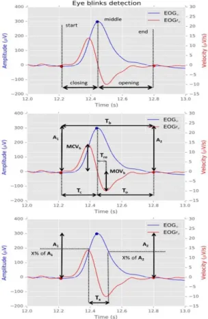
Regarding vertical channels, it is crucial to detect blinks and discard fast vertical movements, called saccades, and other slow movements. The algorithm for blink events detection involves a derivative-based method [33], of which the first step is the computation of the first derivative of the EOGv signal, EOG’v, that can be related to a kind of ‘velocity’ of the signal (amplitude per time unit). Potential blinks are selected through peak detection in the absolute signal of the derivative, and also velocity thresholding, allowing slow movements to be discarded. After that, around those peaks, a change of signal is searched for in the regions before positive peak and after negative peak. These corresponding points in EOGv define the start and the end of a blink. The point where EOG’v reaches zero (middle point) corresponds to the maximum
Table 1 Extracted ECG features
No Feature Description
1 HR Heart rate
2 SDNN Standard deviation of NN intervals (HRVi)
3 SDSD Standard deviation of differences between adjacent NN intervals (HRVi − HRVi−1)
4 RMSSD Square root of the mean of the sum squares of differences between adjacent NN intervals
5 NN50 Number of pairs of successive NNs that differ by more than 50 milliseconds 6 pNN50 NN50 divided by total number of NNs
7 NN20 Number of pairs of successive NNs that differ by more than 20 milliseconds 8 pNN20 NN20 divided by total number of NNs
9 HF Total energy in the high frequency band (0.15 to 0.4 Hz) 10 LF Total energy in the low frequency band (0.04 to 0.15 Hz) 11 VLF Total energy in the very low frequency band (0.003 to 0.04 Hz) 12 TP Total power in all bands (0.003 to 0.4 Hz)
13 HFnu HF normalized (HF divided by the difference between TP and VLF) 14 LFnu LF normalized (LF divided by the difference between TP and VLF) 15 VLFnu VLF normalized (VLF divided by TP)
16 LF/HF Ratio between LF and HF
Table 2 Extracted EOGv features.
No Feature Description
1 Ab Blink amplitude defined as the minimum between A1 and A2
2 E Blink energy defined as
3 MCVb Maximum closing velocity defined as the maximum value of during closing
phase
4 MOVb Maximum opening velocity defined as the maximum value of during opening phase
5 MMCVb Maximum MCVb value in a time interval (two minutes)
6 MMOVb Maximum MOVb value in a time interval (two minutes)
7 Ab/MCVb Ratio between Ab and MCVb
8 Ab/MOVb Ratio between Ab and MOVb
9 ACV Average closing velocity defined as A1/Tc
10 AOV Average opening velocity defined as A2/To
11 Fb Blink frequency defined as the number of detected blinks per time unit (two-minute
intervals)
12 Tb Blink duration defined as the time interval between start and end of a blink
13 Thb Blink half duration defined as the time between half rise and fall amplitudes of a
blink (T50: 50% of A1 and A2)
14 Tc Duration of the closing phase
15 To Duration of the opening phase
16 Tro Time of reopening defined as the difference between the start of the opening phase
and the point of maximum velocity during same phase
6 peak in EOGv. Two phases are present in a blink: a closing phase, between start and middle points (eyes start to close) and an opening phase, between middle and end points (eyes start to open). Since amplitudes measured at the beginning and at the end of a blink remain unchanged, for each i-th potential blink, just the ones that have a value of |EOGv(endi) − EOGv(starti)| below a certain threshold are considered as true blinks. Based on detected events (see Fig. 2.) 17 features are computed for each blink, resulting in 17 averaged features in two-minute windows with no overlap (Table 2).
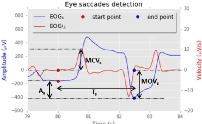
Regarding horizontal channels, EOGh, saccades are detected using a threshold in the velocity signal, EOG’h. Regarding extracted features, two-minute windows were considered. Although these events do not contain a sequence of an eye opening and eye closing (see Fig. 3.), extracted features are similar to the ones related to blinks and are defined in Table 3.
4.2.
Classification
4.2.1 Multimodality
In this work, classification is performed based on three different sets of data: using 16 features from ECG, using 25 features from EOG and using all 41 features from ECG + EOG. These databases were randomly split in a training set (70%) and a test set (30%).
7 4.2.2 Subject-independent classification:
When the division between training set and testing set is done randomly, both datasets have samples corresponding to the same subject and, most likely, samples of all subjects. Thus, when the classifier tries to predict the class of unseen data, it can recognize similar samples seen in the training set. Therefore, this classification is called subject-dependent. Subject-independent classification is performed using as training set the data of n-1 subjects and as testing set the data from the n-th subject. However, data per individual is typically not enough to design a robust model, since each driver is differently affected by sleepiness and, therefore, physiological differences can be really accentuated among drivers.
In this particular case, it would be interesting to create a user-independent system: a warning system that is able to adapt itself to each driver and to learn the user’s behaviour each time the same user drives the vehicle. In practice, the first goal is to design a universal model from data aggregated from many individuals, which is then personalized to each specific individual.
For that purpose, the classifier can learn not only from the data of the n-1 subjects, but also from a small part of the data from the n-th individual, and be tested in the remaining part. This situation is similar to subject-dependent classification, since the user and their features are not completely unknown to the system/classifier. Thus, subject-dependent and subject-independent classifications are performed, using the following scenarios:
• Subject-dependent classification:
- Training and testing sets: split randomly.
- Training set: data from n-1 subjects and 30% of the data from the n-th subject; testing set: 70% data from the n-th subject.
- Training set: data from n-1 subjects and 10% of the data from the n-th subject; testing set: 90% data from the n-th subject.
• Subject-independent classification: Table 3 Extracted EOGh features.
No Feature Description
18 Fs Saccade frequency defined as the number of detected blinks per time unit (two-minute intervals)
19 As Saccade amplitude defined as |EOGh(end) – EOGh (start)|
20 Ts Saccade duration defined as the time interval between start and end of a saccade 21 MCVs Maximum velocity defined as the maximum value of
22 MOVs Maximum velocity defined as the minimum value of 23 MMCVs Maximum MCVs value in a time interval (two minutes) 24 MMOVs Maximum MOVs value in a time interval (two minutes) 25 AV Average velocity defined as the ratio between As and Ts
8 - Training set: data from n-1 subjects and 0% of the data from the n-th subject; testing set: 100% data
from the n-th subject.
KSS ratings collected every fifth minute during the experiments were used as labels. Since several levels of KSS are related to similar states, the KSS ratings can be grouped, either for binary classification (two classes: “awake” - 1 to 6, and “sleepy” - 7 to 9) or for multi-class classification (three classes: “awake” - 1 to 5, “medium” - 6 and 7 and “sleepy” - 8 and 9). This grouping of KSS levels was adopted from previous research [33].
4.2.3 Imbalanced class distributions
The distribution of the classes is illustrated in Fig. 4. Regarding distribution, data can be defined as balanced or imbalanced and the last one is referring to disproportional distributions of one or more classes. For both binary and multi-class classification, “sleepy” is the minority class and “awake” is the majority class. It is plausible to assume that a wrong classification in the “sleepy” class is much more crucial than the inverse case: a driver should always be warned for preventing an accident and there is no danger if the driver is alert and receives a warning.
A classifier “prefers” to correctly classify a higher number of samples of the majority class than a less number of samples of the minority class, leading to a higher misclassification of the “sleepy” class. Several approaches have been proposed for handling these uneven distributions, such as undersampling the majority class and/or creating synthetic data for the minority one [49], or using pairs of observations of opposite classes to build the model, instead of learning from each observation individually [50]. In this work, training is performed with costs, so that the cost of a misclassification in the “sleepy” class is greater than the cost of a misclassification in other classes. A ratio between the number of samples in each class is considered for balancing misclassification costs and therefore, balancing data for each class.
Artificial neural networks (ANN), random forest (RF), support vector machine (SVM) and gradient boosting tree (GBT) were used and, based on accuracy values and 10-fold cross validation, the best combination was selected. This combination includes feature scaling, feature transformation and specific parameters of the classifier.
5. Results and Discussion
5.1.
R-peak detection
Five sessions were randomly selected. For each session, true R peaks were marked and compared with the output of the algorithm, manually. In all five sessions, there were 10 FP (False Positives) and 44 FN (False Negatives) amongst the 34417 R-peaks (sensitivity 99.9%, precision 100.0%).
5.2.
Blink events detection
Three segments of 5 minutes were extracted from the available vertical channels, and blink events were marked manually. The methodology that was used is good enough for getting a good ratio between detected
9 blinks and total of events: in all three sessions, there were 46 FP and 20 FN amongst 427 events (sensitivity 95%, precision 91.3%).
5.3.
Saccade events detection
Three segments of 5 minutes were also extracted from the available horizontal channels and saccade events were marked manually. Similarly to blink detection, this methodology is good enough for getting a good ratio between detected saccades and total of events: there were 1 FP and 5 FN amongst 66 events (sensitivity 92.5%, precision 99.0%).
5.4.
Multimodality
The accuracy from the 2-class and 3-class classifications of sleepiness state for each database (ECG, EOG and ECG + EOG) for SVM, ANN, RF and GBT classifiers are presented in Table 4 as well as the confusion matrices for both settings and GBT classifier.
The results show that the accuracy is improved when a combination of ECG and EOG features are used. That means that, in this case, two sources of information are better than one and there are both ECG and EOG features capable of distinguishing between awake and sleepy states. However, it is possible to conclude that using EOG features alone provides better results than using only the features extracted from ECG signals. GBT and SVM classifiers provided the best results for 2-class and 3-class classifications, respectively, using ECG + EOG information.
For these reasons, these two classifiers are considered in the remaining tests. Feature selection did not improve the results.
5.5.
Subject-independent classification
Tables 5 and 6 present the results obtained with subject-dependent and subject-independent classifications using ECG + EOG database and SVM and GBT classifiers, for 2-class and 3-class problems, respectively. Regarding SVM, for both situations, as expected, results are much better for subject-dependent classification. For subject-independent classification, accuracy values are 56.3% (vs. 87.0%) for two classes and 42.2% (vs. 76.0%) for three classes due to DRawake values, where DR is detection rate. In fact, values of DRsleepy are really low and classification of sleepy states as awake states is significantly higher in subject-independent classification. This means that individual properties of the subjects are really hard to eliminate, being present in the data, and also that sleepiness states does not have the same effect on each subject: the behavior of one sleepy driver is different than the behavior of another. These large individual differences are not new in physiological signals and were already studied regarding ocular metrics [51], [52].
It is important to emphasize that individual differences are not only present in the physiological signals but also in the labels. Labels are based on subjective KSS levels and may vary between drivers: two subjects with similar states can differently evaluate their state by giving different KSS values at a moment. This means, for example, that two labels “medium” and “sleepy” may reflect the same state. By analysing the available samples for each class and for each subject, it was noticed that there was one subject with zero samples in the “sleepy” class, and, for several subjects, the majority class was “sleepy”. Although this situation can be explained because some drivers became sleepy more easily, it may also be explained because there is a discrepancy in the scores given by the drivers. The study presented in [51] that detected large individual differences in ocular metric also used KSS levels as labels.
Regarding GBT, although results are a bit better with this classifier for subject-independent classification (accuracies of 66.3% and 49.9% for GBT classifier vs. 56.3% and 42.2% for the SVM, for two and three classes, respectively), it is possible to infer that the type of the classifier is not an issue in this topic. The
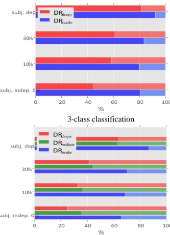
10 classification of the awake class is less problematic (especially in the binary classification), but DRsleepy values decrease severely for both classes and also for DRmedium (values of medium detection rate) values in the 3-class approach. In the training phase, 10% and 30% of the data of the test subject were added. The comparison of all DR values for two and three classes can be seen in the Fig. 5. Basically, with an increase of information of the subject in the training dataset, all DR values are improved. However, regarding “sleepy” class, values near 80% and 60% are achieved in the subject-dependent classification for two and three classes, respectively, which corresponds to a difference of at least 40% and 20% when subject-independent classification is considered. That way, much more data in the training are needed.
5.6.
Imbalanced class distributions
A ratio between the number of samples in each class is considered for balancing misclassification costs and therefore, balancing data for each class. Original results are presented in the upper side of Table 7, and results after the balance can be found in the bottom side, for 2-class and 3-class problems, respectively, using ECG + EOG database.
In fact, based on the results, the SVM classifier is sensitive to imbalanced data. After weight corrections, there were improvements in the classifier regarding the “sleepy” class: from 84.8% to 90.5% for two classes and from 66.3% to 72.2% for three classes. This corresponds to an improvement of almost 6% in DRsleepy for both cases. However, a 5% drop of DRawake, for binary classification,
and a 5% drop of DRmedium and 3% drop of DRawake, for 3-class problem, were also obtained. F1-score is defined as a measure of a test’s accuracy. It is a weighted average of the precision and sensitivity and can be calculated as follows:
𝐹1 = 2Precision + SensitivityPrecision ∙ Sensitivity (1)
Sensitivity measures the proportion of positives that are correctly identified as such and precision the percentage of predictive positives that are truly positive. For the 3-class setting, for each label the metrics (eg. precision, recall, F1) are computed and then these label-wise metrics are aggregated.
For the 2-class problem, the drops mentioned above lead to an increase in F1-score with balanced data for the “sleepy” class but, in general, it decreases (Table 8). For 3-class problem, the F1-score metric decreases for all classes: recall is higher in the “sleepy” class with weight balanced data but precision drops; for the remaining classes, recall is lower and precision drops except for the “awake” class (Table 8).
In this case, of course it is worse to classify “sleepy” as “awake”/“medium” than the opposite but, in fact, for three classes, the percentage regarding awake states classified as sleepy states increased, which is also not acceptable in an alert system.
11 Table 4 Test results (accuracy) of multimodality and confusion matrices for 2-class and 3-class problems using GBT
classifier and ECG, EOG and ECG + EOG features.
Classifier Number of classes ECG EOG ECG + EOG
SVM 2 69.3% 84.5% 87.2% 3 49.3% 69.1% 77.7% ANN 2 68.6% 79.5% 84.0% 3 49.3% 63.3% 59.8% RF 2 69.3% 84.5% 87.4% 3 50.5% 72.7% 74.1% GBT 2 70.3% 86.1% 88.1% 3 52.4% 73.2% 73.9% 2-class 3-class ECG ECG predicted predicted
awake sleepy awake medium sleepy
given awake 84.1% (222) 15.9% (42) given awake 74.1% (143) 21.2% (41) 4.7% (9) sleepy 54.0% (81) 46.0% (69) medium 48.3% (69) 39.2% (56) 12.6% (18) sleepy 39.7% (31) 37.2% (29) 23.1% (18) EOG EOG predicted predicted
awake sleepy awake medium sleepy
given awake 91.3% (264) 8.7% (25) given
awake 88.3% (188) 6.6% (14) 5.2% (11) sleepy 24.3 % (35) 75.7% (109) medium 26.5% (39) 62.6% (92) 10.9% (16)
sleepy 12.3% (9) 37.0% (27) 50.7% (37)
ECG + EOG ECG + EOG
predicted predicted
awake sleepy awake medium sleepy
given awake 59.6% (235) 27.5% (20) given
awake 86.6% (162) 11.8% (22) 1.6% (3) sleepy 54.2% (29) 27.9% (129) medium 24.7% (36) 63.0% (92) 12.3% (18)
12 Table 5 Confusion matrices for 2-class problem using SVM and GBT classifiers and ECG + EOG features.
SVM GBT
Subject-dependent classification Subject-dependent classification
predicted predicted
awake sleepy awake sleepy
given
awake 88.6% (226) 11.4% (29)
given
awake 92.2% (235) 7.8% (20)
sleepy 15.2% (24) 84.8% (134) sleepy 18.4% (29) 81.6% (129)
Subject-independent classification Subject-independent classification
predicted predicted
awake sleepy awake sleepy
given awake 71.7% (34.6) 28.3% (13.6) given awake 80.6% (38.9) 19.4% (9.3)
sleepy 62.4% (17.0) 37.6% (10.3) sleepy 55.3% (16.0) 44.7% (12.9)
Table 6 Confusion matrices for 3-class problem using SVM and GBT classifiers and ECG + EOG features.
SVM GBT
Subject-dependent classification Subject-dependent classification
predicted predicted
awake medium sleepy awake medium sleepy
given awake 90.9% (170) 8.0% (15) 1.1% (2) given awake 86.6% (162) 11.8% (22) 1.6% (3)
medium 21.2% (31) 67.1% (98) 11.6% (17) medium 24.7% (36) 63.0% (92) 12.3% (18)
sleepy 3.8% (3) 30.0% (24) 66.3% (53) sleepy 8.8% (7) 27.5% (22) 63.8% (51)
Subject-independent classification Subject-independent classification
predicted predicted
awake medium sleepy awake medium sleepy
given awake 59.6% (21.8) 27.5% (10.0) 12.9% (4.7) given awake 65.8% (23.7) 26.8% (9.6) 7.5% (2.7) medium 54.2% (13.8) 27.9% (7.1) 17.9% (4.5) medium 47.7% (12.4) 35.9% (9.3) 16.5% (4.3)
13 sleepy awake sleepy medium awake
Fig. 5. Comparing detection rate (DR) values for subject-dependent and subject-independent
classifications.
2-class classification
14 6. Conclusions
Classification of 16 heart and 25 eye-based features from the ECG and EOG signals, respectively, made it possible to monitor driver’s sleepiness state.
Physiological signals are the ones that present the most individual characteristics [53]. For that reason, it is difficult to develop a general and independent classification system. Results showed significantly worse performance in subject-independent classification, especially regarding the “sleepy” class. It is important to emphasize that individual differences are not only present in the physiological signals but also in the labels. The accuracy of the target values, i.e. the reliability of the
Table 7 Confusion matrices for 3-class problem using SVM classifier and ECG + EOG features.
SVM
2-class 3-class
Imbalanced classes Imbalanced classes
predicted predicted
awake sleepy awake medium sleepy
given awake 88.6% (226) 11.4% (29) given awake 90.9% (170) 8.0% (15) 1.1% (2) sleepy 15.2% (24) 84.8% (134) medium 21.2% (31) 67.1% (98) 11.6% (17) sleepy 3.8% (3) 30.0% (24) 66.3% (53)
Balanced classes Balanced classes
predicted predicted
awake sleepy awake medium sleepy
given awake 83.9% (214) 16.1% (41)
given
awake 87.2% (163) 9.6% (18) 3.2% (6) sleepy 9.5% (15) 90.5% (143) medium 19.2% (28) 62.3% (91) 18.5% (27)
sleepy 3.8% (3) 25.3% (20) 72.2% (57)
Table 8 Precision, recall and F1-score metrics for 2-class and 3-class problems using SVM classifier and ECG + EOG features.
2-class 3-class
Imbalanced classes Imbalanced classes
Class Precision Recall F1-score Class Precision Recall F1-score
awake 0.9 0.89 0.9 awake 0.83 0.91 0.87
sleepy 0.82 0.85 0.83 medium 0.72 0.67 0.69 Average 0.87 0.87 0.87 sleepy 0.74 0.66 0.7
Average 0.77 0.78 0.77
Balanced classes Balanced classes
Class Precision Recall F1-score Class Precision Recall F1-score awake 0.93 0.84 0.88 awake 0.84 0.87 0.86 sleepy 0.77 0.91 0.85 medium 0.71 0.62 0.66 Average 0.86 0.87 0.86 sleepy 0.63 0.71 0.67 Average 0.75 0.75 0.75
15 sleepiness ground truth, has an impact on the design and the optimization of the classifiers. Although subjective ratings seem to be the best alternative, especially since KSS is easily applied, unobtrusive, and above all, not much affected by interindividual variations (especially if proper training is provided to the participants) [54], it seems worth to research combinations of different measures (objective measures, for example, lane deviations, biomathematical models of sleepiness, such as the three-process model, and subjective measures, such as KSS, or even a combination of several subjective measures) in real driving conditions. On the other hand, applying methods for imbalanced distributions can be a promising approach.
Further developments in the field should consider more complex machine learning methods better suited to deal with imbalanced data. For example, oversampling of the minority class can be performed to deal with imbalanced class distributions. Also, the length of the 2-minute time window that is used when extracting the features should be investigated further. Different window lengths should be assessed in order to test if this parameter is capable of improving the classification results.
7. Acknowledgments
The work was carried out in collaboration with the ADAS&Me project which is funded by the European Union’s Horizon 2020 research and innovation programme under grant agreement No 688900. The SleepEye dataset was collected within the competence centre ‘Virtual Prototyping and Assessment by Simulation’, which is financed by the Swedish Governmental Agency for Innovation Systems (grant number 2011-03994).
8. References
[1] World Health Organization, ‘Global status report on road safety’ (WHO, 2015).
[2] The Royal Society for the Prevention of Accident, ‘Road Accidents: A Literature Review and Position Paper’ (RoSPA, 2001).
[3] National Highway Traffic Safety Administration, ‘Traffic Safety Facts: A compilation of motor vehicle crash data from the fatality analysis reporting system and the general estimates system’ (National Highway Traffic Safety Administration, 2014).
[4] National Highway Traffic Safety Administration, ‘Traffic Safety Facts: a brief statistical summary. Drowsy driving’ (National Highway Traffic Safety Administration, 2011).
[5] Sahayadhas, A., Sundaraj, K., Murugappan, M.: ’Detecting driver drowsiness based on sensors: a review’, Sensors, 2012, 12, (12), pp. 16937-16953.
[6] Yu, X.: ‘Real-time Nonintrusive Detection of Driver Drowsiness’. University of Minnesota Center for Transportation Studies, 2009.
[7] Brown, I.: ‘Driver fatigue’, Human Factors: The Journal of the Human Factors and Ergonomics Society, 1994, 36, (2), pp. 298–314.
[8] Wang, M., Jeong, N.,Kim, K., et al.: ‘Drowsy behavior detection based on driving information’, International Journal of Automotive Technology, 2016, 17, (1), pp. 165-173.
[9] Wu, Q., Zhao, Y., Bi, X.: ‘Driving fatigue classified analysis based on ecg signal’, Fifth International Symposium on Computational Intelligence and Design, 2012, 2, pp. 544–547.
[10] Vicente, J., Laguna, P., Bartra, A., et al.: ‘Drowsiness detection using heart rate variability’, Medical & biological engineering & computing, 2016, pp. 1–11.
[11] Rodríguez-Ibáñez, N., García-González, M. A., Fernández-Chimeno, M., et al: ‘Drowsiness detection by thoracic effort signal analysis with professional drivers in real environments’, Engineering in Medicine and Biology Society, EMBC, Annual International Conference of the IEEE, August 2011, pp. 1–25.
[12] Yu, X. B.: ‘Non-Contact Driver Drowsiness Detection System’ (Safety IDEA Project 17, 2012).
[13] Lenné, M. G., Jacobs, E. E.: ‘Predicting drowsiness-related driving events: a review of recent research methods and future opportunities’, Theoretical Issues in Ergonomics Science, 2016, 17, (5-6), pp. 533-553.
[14] Hallvig, D., Anund, A., Fors, C., Kecklund, G., et al.: ‘Sleepy driving on the real road and in the simulator—A comparison’, Accident Analysis & Prevention, 2013, 50, pp. 44-50.
[15] Vicente, J., Laguna, P., Bartra, A., et al.: ‘Detection of driver’s drowsiness by means of hrv analysis’, Computing in Cardiology IEEE, 2011, pp. 89–92.
[16] Wang, J. S., Chung, P. C., Wang, W. H., et al: ‘Driving conditions recognition using heart rate variability indexes’, Sixth International Conference on Intelligent Information Hiding and Multimedia Signal Processing IEEE, 2010, pp. 389–392. [17] Gupta N., ‘Ecg and wearable computing for drowsiness detection’. PhD thesis, California State University, Northridge,
2014.
[18] Rigas, G., Goletsis, Y., Bougia, P., et al.: ‘Towards driver’s state recognition on real driving conditions’, International Journal of Vehicular Technology, 2011, 2011, pp. 1-14.
[19] Mårtensson, H., Keelan, O., Ahlström, C.: ‘Driver Sleepiness Classification Based on Physiological Data and Driving Performance From Real Road Driving’, IEEE Transactions on Intelligent Transportation Systems, 2018, pp. 1-10. [20] Healey, J. A., Picard, R. W.: ‘Detecting stress during real-world driving tasks using physiological sensors’, IEEE
Transactions on Intelligent Transportation Systems, 2005, 6, (2), pp. 156–166.
[21] Miyaji, M.: ‘Method of drowsy state detection for driver monitoring function’, International Journal of Information and Electronics Engineering, 2014, 4, (4), pp. 264-268.
[22] Begum, S., Ahmed, M. U., Funk, P., et al: ‘Mental state monitoring system for the professional drivers based on heart rate variability analysis and case-based reasoning’, Computer Science and Information Systems, 2012, pp. 35-42.
16 [23] Jung, S. J., Shin, H. S., Chung, W. Y.: ‘Driver fatigue and drowsiness monitoring system with embedded
electrocardiogram sensor on steering wheel’, IET Intelligent Transport Systems, 2014, 8, (1), pp. 43–50.
[24] Patel, M., Lal, S., Kavanagh, D., et al: ‘Applying neural network analysis on heart rate variability data to assess driver fatigue’, Expert systems with Applications, 2011, 38, (6), pp. 7235–7242.
[25] Murata, A. M., Hiramatsu, Y.: ‘Evaluation of drowsiness by hrv measures - basic study for drowsy driver detection’, Fourth International Workshop on Computational Intelligence & Applications, 2008.
[26] Roy, R., Venkatasubramanian, K.: ‘Ekg/ecg based driver alert system for long haul drive’, Indian journal of science and Technology, 2015, 8, (19).
[27] Camm, A. J., Malik, M., Bigger, J., et al: ‘Heart rate variability: standards of measurement, physiological interpretation and clinical use. Task force of the european society of cardiology and the north american society of pacing and electrophysiology’, Circulation, 1996, 93, (5), pp. 1043–1065.
[28] Khushaba, R. N., Kodagoda, S., Lal, S., et al: ‘Driver drowsiness classification using fuzzy wavelet-packet-based feature-extraction algorithm’, IEEE Transactions on Biomedical Engineering, 2011, 58, (1), pp. 121–131.
[29] Shinar, Z., Akselrod, S., Dagan, Y., et al: ‘Autonomic changes during wake-sleep transition: A heart rate variability based approach’, Autonomic Neuroscience, 2006, 130, (1), pp. 17–27.
[30] Awais, M., Badruddin, N., Drieberg, M.: ‘A non-invasive approach to detect drowsiness in a monotonous driving environment’, TENCON 2014 IEEE Region 10 Conference, 2014, pp. 1-4.
[31] Jammes, B. Sharabty, H., Esteve, D.: ‘Automatic eog analysis: A first step toward automatic drowsiness scoring during wake-sleep transitions’, Somnologie-schlafforschung und Schlafmedizin, 2008, 12, (3), pp. 227–232.
[32] Yue, C.: ‘Eog signals in drowsiness research’. PhD thesis, Linköping University, 2011.
[33] Ebrahim, P.: ‘Driver drowsiness monitoring using eye movement features derived from electrooculography’. PhD thesis, University of Stuttgart, 2016.
[34] Rodríguez-Ibáñez, N., Meca-Calderón, P., García-González, M. A., et al: ‘Drowsiness detection by electrooculogram signal analysis in driving simulator conditions for gold standard signal generation’, Proceedings of the International Conference on Biomedical Electronics and Devices, 2013, 1, pp. 57–63.
[35] Pettersson, K., Jagadeesan, S., Lukander, K., et al: ‘Algorithm for automatic analysis of electro-oculographic data’, Biomedical engineering online, 2013, 12, (1), pp. 110.
[36] Gao, X. Y., Zhang, Y. F., Zheng, W. L., et al: ‘Evaluating driving fatigue detection algorithms using eye tracking glasses’, 7th International IEEE/EMBS Conference on Neural Engineering, 2015, pp. 767–770.
[37] Hu, S., Zheng G.: ‘Driver drowsiness detection with eyelid related parameters by support vector machine’, Expert Systems with Applications, 2009, 36, (4), pp. 7651-7658.
[38] Lal, S., Craig, A.: ‘A critical review of the psychophysiology of driver fatigue’, Biological psychology, 2001, 55, (3), pp. 173–194.
[39] Lee, M. L., Howard, M. E., Horrey, W., et al.: ‘High risk of near-crash driving events following night-shift work’, Proceedings of the National Academy of Sciences, 2016, 113, (1), pp. 176-181.
[40] Ftouni, S., Sletten, T. L., Howard, M., et al.: ‘Objective and subjective measures of sleepiness, and their associations with on-road driving events in shift workers’, Journal of sleep research, 2013, 22, (1), pp. 58-69.
[41] Li, G., Chung, W. Y.: ‘A context-aware EEG headset system for early detection of driver drowsiness’, Sensors, 2015, 15, (8), pp. 20873–20893.
[42] Picot, A., Charbonnier, S., Caplier, A.: ‘On-line detection of drowsiness using brain and visual information’, Transactions on systems, man, and cybernetics-part A: systems and humans, May 2012, 42, (3), pp. 764–775.
[43] Jirina, M., Bouchner, P., Novotny, S.: ‘Identification of driver’s drowsiness using driving information and EEG’, Neural Netw. World, 2010, 20, (6), pp. 773–791.
[44] Li, G., Lee, B. L., Chung, W. Y.: ‘Smartwatch-based wearable EEG system for driver drowsiness detection’, IEEE Sensors Journal, 2015, 15, (12), pp. 7169–7180.
[45] Ahlstrom C., Fors, C., Anund, A. et al.: ‘Video-based observer rated sleepiness versus self-reported subjective sleepiness in real road driving’, European Transport Research Review, 2015, 7, (4), pp. 38.
[46] Doran, S. M., Van Dongen, H. P. A., Dinges, D. F.: ‘Sustained attention performance during sleep deprivation: evidence of state instability’, Archives italiennes de biologie, 2001, 139, (3), pp. 253-267.
[47] Ǻkerstedt, T., Gillberg, M.: ‘Subjective and objective sleepiness in the active individual’, International Journal of Neuroscience, 1990, 52, (1-2), pp. 29–37.
[48] Fors, C., Ahlström, C., Sörner, P., et al.: Camera-based sleepiness detection: final report of the project SleepEYE, The Swedish National Road and Transport Research Institute, 2011.
[49] Chawla, N. V., Bowyer, K. W., Hall, L. O., et al.: ‘SMOTE: synthetic minority over-sampling technique’, Journal of artificial intelligence research, 2002, 16, pp. 321-357.
[50] Cruz, R., Fernandes, K., Cardoso, J. S., et al.: ‘Tackling class imbalance with ranking’, In Neural Networks (IJCNN), 2016 International Joint Conference, July 2016, pp. 2182-2187.
[51] Ingre, M., Åkerstedt, T., Peters, B., et al.: ‘Subjective sleepiness, simulated driving performance and blink duration: examining individual differences’, Journal of sleep research, 2006, 15, (1), pp. 47-53.
[52] Chua, E. C. P., Yeo, S. C., Lee, I. T. G., et al.: ‘Individual differences in physiologic measures are stable across repeated exposures to total sleep deprivation’, Physiological reports, 2014, 2, (9).
[53] Sparrow, A. R., LaJambe, C. M., Van Dongen, H. P. A.: ‘Drowsiness measures for commercial motor vehicle operations’, Accident Analysis & Prevention, 2018.
17 [54] Åkerstedt, T., Anund, A., Axelsson, J. et al.: ‘Subjective sleepiness is a sensitive indicator of insufficient sleep and