Mälardalen University Press Licentiate Theses No. 90
WATER CONTENT MEASUREMENT IN WOODY BIOMASS
USING DIELECTRIC CONSTANT AT RADIO FREQUENCIES
Ana Marta Marques Duarte da Paz 2008
Copyright © Ana Marta Marques Duarte da Paz, 2008 ISSN 1651-9256
ISBN 978-91-86135-01-0
Printed by Arkitektkopia, Västerås, Sweden
Water content measurement in woody
biomass using dielectric constant
at radio frequencies
Ana Marta Marques Duarte da Paz
2008
Summary
The desire to replace of fossil fuels has increased the use of woody biomass as fuel in heating and power plants. An important parame-ter for the use of woody biomass as fuel is its waparame-ter content, as this influences the heating value and thereby the combustion control and fuel pricing. Currently, water content is determined using the gravi-metric method by drying samples in an oven. This method is neither fast nor representative, as the water content can vary largely in differ-ent parts of the container. A need has thus arisen to develop sensors that are able to measure water content of biomass on-line and in a representative way.
This thesis presents results from studies on the measurement of the water content of woody biomass using radio frequencies. Included are studies on the influence of temperature on the measurements; the use of dielectric mixing models to explain the dielectric behavior of woody biomass and the application of the measurement principle to full-scale.
It was found that varying the temperature between 1 and 62did not
influence the prediction of water content in biomass. It was possible to explain the behavior of the dielectric constant of woody biomass with a model with a physical basis using empirically obtained parameters. Applying the principle full-scale had positive results but showed a larger prediction error than laboratory-scale measurements.
Sammanfattning
N¨ar v¨armeverk och kraftv¨armeverk runt om i v¨arlden b¨orjade se sig
omkring efter alternativ till de fossila br¨anslena s˚a ledde detta till
en snabb ¨okning i anv¨andningen av biobr¨anslet. Vatteninneh˚allet
i biobr¨anslet ¨ar en viktig parameter f¨or f¨orbr¨anningsanl¨aggningar
eftersom fukten i materialet p˚averkar v¨armev¨ardet och d¨armed ¨aven
f¨orbr¨anningsprocessen och priset f¨or biobr¨anslet. Idag fastst¨alls bio-br¨anslet fukthalt med en gravimetrisk metod, d.v.s. genom torkning
och v¨agning av br¨anslet. Detta ¨ar en l˚angsam metod som inte ger
en representativ bild av hur fukthalten varierar i en s¨andning,
fuk-thalten kan n¨amligen variera mycket beroende p˚a var och hur provet
tas. Denna os¨akerhet har ¨okat behovet av att utveckla sensorer som
kan avl¨asa vatteninneh˚allet p˚a ett snabbt s¨att och ¨aven ge resultat
representativa f¨or hela volymen.
Den h¨ar rapporten presenterar resultaten fr˚an studier av en typ av
fukthaltsm¨atningar p˚a biobr¨ansle d¨ar vattenhalten best¨ams med hj¨alp
av radiov˚agor. Studien inneh˚aller en unders¨okning av hur
tempera-turen kan p˚averka m¨atningarna, anv¨andandet av dielektriska
mod-eller f¨or att f¨orklara det dielektriska beteendet hos biobr¨asnle samt
att tekniken har till¨ampats p˚a en f¨orbr¨anningsanl¨aggning i ett
full-skaligt f¨ors¨ok.
Studien visar p˚a att varierande temperaturer mellan 1 och 62 inte
har n˚agon p˚averkan p˚a resultaten fr˚an fukthaltsm¨atningarna p˚a bio-br¨ansle. Det var ¨aven m¨ojligt att beskriva dielektriska konstant i biobr¨ansle med en fysikaliskt baserad modell med empiriska
parame-trar. Det fullskaliga f¨ors¨oket visade p˚a goda resultat men med st¨orre
Aknowledgments
There are several people responsible for me starting the work on this thesis. The most decisive of all was undoubtedly my main supervi-sor Professupervi-sor Erik Dahlquist, to whom I would like to thank for the support and confidence during this period.
I would also like to thank my co-supervisor and friend Jenny Nystr¨om for helping me in all possible ways at work and personally, and my co-supervisor Eva Thorin for support and exhaustive work as a co-author in my papers.
My appreciation also goes to Clarke Topp who lead me into the way of physics and who was untiring as a co-author in our paper.
The projects that resulted in this thesis were supported by the Ther-mal Engineering Research Institute, V¨armef¨orsk, and the Swedish Energy Agency, Energimyndigheten, to whom I would like to thank. I would like to thank the support from the staff at the Eskilstuna En-ergy and Environment heating and power plant. I am specially grate-ful to my colleagues, who gave their precious help with the grate-full-scale measurements: Bijan, Weilong, Christer, Fredrik, Iana, Eva, Jenny, and Hamid. Thanks also to Johan for the help with the Swedish text. I would also like to thank Stefan Backa, Magnus Otterskog, and Nikola Petrovic, for the interesting discussions we had and their help in the measurements.
Finally, I thank all my friends in Portugal and elsewhere around the world, since I could only be here and do this work knowing they are there each time I return! I want to thank Tiago, not only for being the most important in my life, but also for all the help and talks around this work!
Papers included in this thesis Paper I
A Paz, J Nystr¨om and, E Thorin. Influence of temperature in radio frequency measurements of moisture content in biofuel. In Proceed-ings of IMTC 06, IEEE Instrumentation and Measurement Technol-ogy Conference, pages 175-179, Sorrento, Italy, 2006.
Paper II
A Paz, E Thorin and, C Topp. Dielectric Mixing models for water content measurement in woody biomass. Submitted to Bioresource Technology Journal on 5 March 2008, revised on August 2008.
Paper III
A Paz, E Thorin, and E Dalquist. A new method for bulk measure-ment of water content in woody biomass. In Proceedings of Ecowood 08, 3rd Conference on Environmental Compatible Forest Products, Porto, Portugal, 2008.
I have been the main author in all papers. Jenny Nystr¨om and Eva Thorin have made the measurement planning in Paper I. Clarke Topp contributed to the initial idea and was the initial driving force behind the study in Paper II.
Symbols and abbreviations
used in the thesis
Symbols
ǫ relative complex permittivity ǫ′
relative dielectric constant ǫ′′
relative dielectric loss factor
ǫ0 permittivity of the free space [F·m
−1
] ǫ′
∞ relative dielectric constant at infinite hight frequencies
ǫ′
m relative dielectric constant of the mixture
ǫ′
i relative dielectric constant of the component i in the mixture
ǫ′
st relative static dielectric constant
θi volumetric content of the component i of the mixture
θw volumetric content of total water phase
µ relative permeability
µ0 permeability of the free space [H·m
−1
]
ρw water density [Kg·m
−3
]
ρt density of the sample [Kg·m
−3
]
σ conductivity [S·m−1
] τ relaxation time [s]
ω angular frequency [rad·s−1
] B magnetic flux density [T]
c electromagnetic wave velocity in free space [m·s−1
]
D electrical flux density [C·m−1
]
Dpi depolarization factor for the component i in a mixture
E electrical field strength [V·m−1
]
J current density [A·m−2
]
H magnetic field strength [A·m−1
j square root of -1
Ms mass of dry phase [Kg]
Mt total mass of the sample [Kg]
Mw mass of total water phase [Kg]
M Cw water content based on mass of the total sample [%]
M Cd water content based on mass of the dry sample [%]
v electromagnetic wave velocity in a material [m·s−1
]
Vt total volume of the sample [m
3
]
Vw volume of the total water phase [m
3
] Abbreviations
GPR ground penetrating radar MG Maxwell-Garnett model
PLS partial least square regression PS Polder van Santen model
RMSE root mean square error RF radio frequency
TDR time domain reflectometry
List of Figures
1.1 Diagram of the structure of this thesis. . . 21
2.1 The ǫ of free water at 0, 20 and 60 as a function of
frequency. . . 28
2.2 The ǫ of the wood cell wall substance at the
tempera-ture 20-25 as a function of frequency. . . 30
2.3 The ǫ′
of free water, oven-dry wood, wood with M Cd=30%
and wood M Cd=100%, for a frequency of 10
8
Hz, and
as a function of temperature . . . 32
2.4 Diagram of the laboratory-scale measurement system. . 37
3.1 The ǫ′
m of woody biomass as a function of temperature. 41
3.2 The ǫ′
m of woody biomass as a function of different
water content definitions. . . 43
Contents
1 Introduction 17 1.1 Problem definition . . . 18 1.2 Objectives . . . 19 1.3 Methodology . . . 19 1.4 Thesis outline . . . 212 Background and related work 23 2.1 Electromagnetic properties . . . 23
2.2 Permittivity . . . 25
2.2.1 Polarization phenomena . . . 26
2.2.2 Permittivity of water . . . 27
2.2.3 Permittivity of wood . . . 29
2.2.4 Permittivity of moist wood . . . 30
2.3 Water content . . . 32
2.3.1 The relationship between water content and di-electric properties . . . 32
2.3.2 Reference water content . . . 34
2.3.3 Water content definitions . . . 34
2.4 Measurement systems . . . 35
2.4.1 Laboratory-scale system for bulk measurements of woody biomass . . . 37
3 Contributions of the thesis 39
3.1 Influence of temperature in the ǫ′
m of
woody biomass . . . 39
3.1.1 Results and discussion . . . 40
3.2 Dielectric Mixing models . . . 41
3.2.1 Results and discussion . . . 43
3.3 Full-scale measurements . . . 44
3.3.1 Results and discussion . . . 46
4 Conclusions 47 5 Future work 49 Bibliography . . . 51
Appended Papers . . . 54
Chapter 1
Introduction
The replacement of fossil fuels by renewables is a current demand all over the world. This is mainly due to the contribution of fossil fuels to the greenhouse effect and the resulting climate changes, as well as a desire to improve security of energy supply. The goal of the European Union is that 12% its energy should come from renewable sources by 2010. The potential biomass quota is estimated at 8% [1].
The use of woody biomass has been found especially successful in heating and combined heat and power plants in countries with large woody feedstock. In Sweden biomass represents 7.8% of the electricity production and 65% of the heating production. It contributes to 18.6% of the total energy supply [2].
The problem of bulk measurement of water content in woody biomass has been raised by the energy sector. The water content of biomass is important for the runnability of the plants as it influences the heating value and thereby the combustion control and fuel pricing. Currently, water content is determined using the standard gravimetric method by drying samples in an oven. The drying time can be up to 24 hours and the samples are taken from the surface of the biomass in the con-tainers. The method is therefore neither fast nor representative, as the water content can vary largely between different parts of the con-tainer. This has given rise to the need to develop sensors that are able to measure water content of biomass on-line and in a representative way [3].
The biomass arrives at the plants in containers transported by trailer trucks. At the entrance the biomass delivery is registered and weighed, the volume is estimated and samples for water content determination are taken. The biomass is then tipped on the ground at the plant or directly on a hopper from where conveyor belts transport it to the boiler. To develop a method that would be able to measure water con-tent directly in containers arriving at the plants and giving immediate results, would facilitate the decision as to where to tip the biomass. Results should also be representative for the volume of biomass in the container.
There are on-line methods for measuring of water content of woody biomass in conveyor belts using different techniques, such as as near infrared spectroscopy (NIR) [4] and nuclear magnetic resonance (NMR) [5]. A review of the methods for determining water content in wood-chips is presented by [3]. There are also several measurement ap-plications for water measurement in different materials at microwave frequencies [6]. However, none of these methods are able to perform a bulk measurement as described above.
Nystr¨om [7] developed a method to perform bulk measurements of water content in woody biomass. This method uses radio frequency (RF) waves which have large wavelength and therefore are able to travel longer in a material as they suffer less attenuation. The method
is able to measure 0.1 m3
of biomass using a circular sample holder with a diameter of about 0.6 m and a fuel depth of about 0.4 m. The measurements are done accessing only one side of the biomass and use reflection data. The setup included an antenna on the top of the material which emits the waves. The waves travel through the mate-rial, suffer total reflection at the bottom of the metallic container, and travel back to the antenna. This method pointed out a measurement principle possible that can be applied in measuring biomass directly in the transport containers upon arrival at the plants.
1.1
Problem definition
The measurement principle developed by Nystr¨om offers different re-search challenges. As the dielectric properties of woody biomass have
not been previously studied several questions about the dielectric measurements were to be answered. These questions were mainly related to the relationship between water content and the dielectric measurements and the influence of other parameters such as tem-perature or density in that relationship. The ultimate challenge was its application to the measurement of water content directly in the containers in which biomass is transported by the truck trailers.
1.2
Objectives
The general aim of this thesis is to provide deeper understanding of the dielectric properties of woody biomass and make use of this knowledge in practical applications for water content measurement. The following questions were specifically investigated:
- how does the sample temperature influence the measurement of water content in woody biomass? (Paper I)
- can the dielectric constant estimated from the measurements of woody biomass be described by a dielectric mixing model? (Paper II)
- can the estimate of the dielectric constant be used for water content prediction? (Paper II)
- how can the measurement principle be applied to full-scale system? (Paper III)
1.3
Methodology
Woody biomass as considered in this study consists of different types of biomass derived from forest products. These are comprised mainly of wood, but also of treetops and bark. The samples can be wood-chips, sawdust from sawmills, residual woodchips from destruction of pallets or other constructions, which usually have very low water con-tent, or mixtures of wood, treetops and bark. These materials have their origin mainly in willow, spruce and pine. These are the most
common materials used as biofuels in heating and power plants in Sweden.
Two different measurement systems were used to perform the mea-surements. The results in Paper I and Paper II were obtained with measurements made with a laboratory-scale measurement setup de-veloped by Nystr¨om [7]. This method is briefly described in section 2.4.1 of this thesis. The results in Paper III were obtained with a full-scale measurement system that is described in more depth in [8]. Both measurement systems aim at using information from the whole depth of material and use a RF antenna situated above the fuel. The antenna emits waves that travel through the material, are reflected at the bottom of the sample holder and back to the antenna. Both methods use reflection data in time-domain to correlate with water content. The use of signal in the time-domain allows identification of the bottom reflection. The difference between the two methods is that the laboratory-scale method used a sweep of frequencies be-tween 310 and 800 MHz emitted by a log antenna, while the full-scale method used a ground penetrating radar system (GPR) composed of emitter and receiver antennas with a center frequency of 250 MHz. The other main difference is that in the laboratory-scale method the sample was inside a construction made of two steel drums that worked as a wave-guide. In the full-scale method the setup is an open-air one, as the GPR antenna is placed on top of the biomass in its transport container. Open-air systems are more complex than systems using guided waves.
There are also different methods used to correlate the dielectric mea-surements of woody biomass with water content. In Paper I a statis-tical model was built using a multivariate data analysis method. Par-tial least square regression (PLS) was used to correlate the reflection time-domain signal with the water content. The thesis also presents the results on the influence of temperature using the dielectric con-stant calculated from the wave velocity. In Paper II and Paper III the dielectric constant of woody biomass is calculated using the wave velocity in the samples. In Paper II physically based models are used to relate the dielectric constant with water content. In Paper III the dielectric constant is related with water content using curve fitting. The PLS models were built using the multivariate data analysis
gram The Unscrambler® (v 9.7, CAMO, Norway). All other models
were built using Matlab® (R2007b, The Mathworks, USA).
The use of the dielectric constant to predict water content is advan-tageous because such a relation can be used in different applications even if different setups or amounts of material are used. If PLS mod-els are used, it might be necessary to carry out new calibration for a different measurement setup.
1.4
Thesis outline
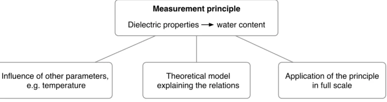
This thesis is based on the contribution of three scientific papers. Figure 1.1 schematizes how the different research papers relate in this thesis. The water content measurement principle using the dielectric properties of woody biomass at radio frequencies is common to all the studies. Paper I studies the influence of temperature on the relation-ship between water content and dielectric measurements. Paper II used the measurements to estimate the dielectric constant of biomass and attempts to explain the relation between the dielectric constant and water content using a physical model. It also verified the use of this model to predict water content in biomass samples. Paper III presents results of the application of the method to full-scale and com-pares the relation between the dielectric constant and water content with the relation obtained in laboratory measurements.
Measurement principle
Dielectric properties water content
Theoretical model explaining the relations Influence of other parameters,
e.g. temperature
Application of the principle in full scale
Figure 1.1: Diagram of the structure of this thesis.
In this introduction the general background to the project is presented as well as the objectives and a general description of the methodology used in the papers.
Chapter 2 presents background theory and related work of importance for the discussion of the results. This includes a short presentation of how electromagnetic waves interact with materials. The dielectric behavior of wood, water and moist wood and its dependence on fre-quency and temperature are also presented, based on bibliographic data. This is followed by a discussion on models relating the dielec-tric properties and water content, the standard measurement of water content and different water content definitions. Finally a brief pre-sentation is given on water content measurement systems that can be related with the project.
Chapter 3 returns to the contributions of the three papers and dis-cusses the results achieved against a background of the knowledge presented in Chapter 2.
The conclusions and future work are presented in Chapters 4 and 5.
Chapter 2
Background and related
work
This chapter is divided in four main sections. In the first a short summary is given of the theory of electromagnetic waves interaction with materials. In the second section the permittivity of water, wood and moist wood and its behavior are discussed as a background to the thesis’ contributions. In the third section methods are presented for the determination of water content from dielectric measurements, along with different water content definitions. In the last section different measurement systems are discussed.
2.1
Electromagnetic properties
Considering their interaction with electromagnetic fields, materials can be classified as high-conductivity and low-conductivity materials. In high conductivity materials, or conductors, such as metals, the penetration depth of the electromagnetic waves is very small, and an incident wave results in a reflected wave radiated by the current induced in the material. In low-conductivity materials, or insulators, the electrons in the outer orbits of the atoms are very stable and are not easily liberated even under the application of an external electric field. Electromagnetic waves propagate inside dielectrics and suffer different phenomena such as delay and attenuation [9], [10].
In this thesis woody biomass is discussed as a mixture of air, water and wood, which are dielectric materials. Citing Von Hippel [11], dielectrics are ”not a narrow class of so-called insulators, but the broad expanse of nonmetals considered from the standpoint of their interaction with electric, magnetic, of electromagnetic fields. Thus we are concerned with gases as well as with liquids and solids, and with the storage of electric and magnetic energy as well as its dissipation.” The interactions between electromagnetic fields and materials are de-scribed by the Maxwell equations from which the following constitu-tive equations can be derived [12]:
D = ǫE (2.1)
B = µH (2.2)
J = σE (2.3)
where E is the electrical field strength, D the electrical flux density, H the magnetic field strength, B the magnetic flux density and J current density. Permittivity ǫ, permeability µ and conductivity σ are the electromagnetic constitutive parameters of materials and describe their electromagnetic properties [9], [12].
Permittivity describes the interaction of a material with the electrical field. It is a measure of how much the electric charge distribution of the material is changed, or polarized, by application of an electri-cal field [13]. Polarization phenomena are described further in sec-tion 2.2.1. Permeability describes the interacsec-tion of a material with the magnetic field. It is a measure of the magnetization, or rinse of magnetic moments in a material with an applied magnetic field [12]. All materials respond to magnetic fields to some degree. However, in most materials, permeability does not vary significantly from that of the free space and is therefore not considered when making electro-magnetic measurements [10]. The conductivity characterizes the ease with which charges can move freely in a material. The conductivity of dielectrics is also small. Thus, permittivity becomes the main pa-rameter used for characterizing dielectrics and will therefore be the electromagnetic property discussed in the next sections.
2.2
Permittivity
Permittivity and permeability of materials is most commonly ex-pressed in relation to the permittivity of free space, and therefore named relative permittivity. In this thesis and in the appended pa-pers, whenever ǫ and µ are named they refer to the relative per-mittivity and permeability. The only exception to this is made in equation 2.1 and 2.2, where the absolute permittivity and absolute permeability are represented.
Electromagnetic fields interact with the material with energy storage and energy dissipation phenomena. Energy dissipation occurs when the material absorbs electromagnetic energy and storage when there is no loss in the energy change between field and material. Therefore permittivity is expressed as a complex number:
ǫ = ǫ′
− jǫ′′ (2.4)
where the real part ǫ′
is the relative dielectric constant describing the
energy storage, and the imaginary part, ǫ′′
is the relative dielectric loss
factor which represents the energy losses. ǫ′
changes the rate between the electric and magnetic field strengths, or impedance, and decreases
the velocity of propagation and the wavelength. ǫ′′
represents the power that is absorbed by the material, or the rate of attenuation in
the material. To a first order approximation, ǫ′′
does not influence the velocity of a propagating wave [10].
The velocity of propagation of electromagnetic waves in free space, c, is:
c = õ1
0ǫ0
(2.5)
where ǫ0 is the permittivity of the free space equal to 1/36π·10
−9
Fm−1
and µ0 is the permeability of the free space equal to 4π · 10
−7
Hm−1
which are universal constants, c then becomes 2.998·108
ms−1
[14]. In a similar way, the velocity of the electromagnetic waves in a mate-rial, v, can be calculated using the permittivity and permeability of the material relative to that of free space:
When ǫ′′
/ǫ′
≪1, the medium is called a low-loss dielectric, allowing for
the approximation ǫ ≈ ǫ′
[12]. Also, for most non magnetic materials the relative permeability is equal to 1. This allows equation 2.6 to be simplified, resulting in equation 2.7:
v = √c
ǫ′ (2.7)
Although the previous approximation can be done for low-loss mate-rials, the effect of the imaginary part of permittivity can be present
in the estimate of ǫ′
. Some authors have named the parameter ǫ′
as calculated with equation 2.7 the apparent dielectric constant [15] or apparent permittivity [16].
2.2.1
Polarization phenomena
Permittivity can be understood as a measure of the polarization that occurs in a medium when it is submitted to an electrical field. Po-larization arises from a variety of physical phenomena. In the next paragraphs the polarization phenomena of interest to this thesis are
described. Ionic polarization, which only influences ǫ′′
, is not further described because woody biomass is considered as a low-loss dielectric (see section 2.2.4).
Electronic and atomic polarization
Electronic and atomic polarization are similar in nature. Electronic polarization arises from the shifts in the electron orbits relative to the nucleolus of the atoms under the influence of an electric field. Atomic polarization arises from the shifts in the positions of ions in molecules [10].
Electrons, atoms and dipoles require a certain time to return to initial position after the application of an electric field. This period of time is called the relaxation time, τ . The frequency with a period equal to τ is called the relaxation frequency and for this frequency the polarization has a maximum [13]. At higher frequencies than the relaxation frequency losses start to occur, ǫ′
decreases and ǫ′′
increases. 26
Since the inertia of electrons and atoms is very small these type of polarization are the first to develop in a material when an electric field is applied and the relaxation frequency is rather high, in the visible light region. If only these two polarization mechanisms are present the material has small losses at RF [10].
Dipole polarization
Dipole or orientation polarization is the alignment of dipoles of mo-lecules with permanent dipole with the electric field. This type of polarization needs longer than electronic and atomic polarization to be able to develop completely. The τ for the molecules is longer and the relaxation frequency is consequently lower [17].
2.2.2
Permittivity of water
The water molecule has a permanent dipole moment due to its posi-tively charged hydrogen atoms and negative oxygen atom. The polar
nature of the water molecule is responsible for its large ǫ′
at fre-quencies under the water molecule relaxation frequency, where dipole polarization occurs.
Variation with frequency
The permittivity of polar substances can be described by the Debye relation: ǫ = ǫ′ ∞ + ǫ′ st − ǫ ′ ∞ 1 + jωτ (2.8) where ǫ′
∞ is the permittivity at infinitely high frequencies for which
dipole polarization has no time to develop, ǫ′
st is the static permittivity
corresponding to the permittivity at low frequencies, where dipole polarization develops fully and ω is the angular frequency.
Figure 2.1 shows the variation of the relative complex permittivity, ǫ, of water with frequency, according to equation 2.8. The black lines
represent the ǫ of water at 20 . Looking at this temperature it can
be noticed that the real part of permittivity, ǫ′
, is constant at fre-quencies higher and lower than the relaxation frequency. While at
108 109 1010 1011 10 20 30 40 50 60 70 80 frequency Hz ε ε’ 0°C ε’’ 0°C ε’ 20°C ε’’ 20°C ε’ 60°C ε’’ 60°C
Figure 2.1: The ǫ of free water at 0, 20 and 60 as a function of
frequency. The complex permittivity was calculated using the Debye equation with parameter values published by [18].
low frequencies ǫ′
is 80 due to the presence of dipole polarization, its
value is much lower above 1011
Hz. At higher frequencies the
orien-tation of the dipoles no longer contributes to ǫ′
, a phase lag between the field and the dipole orientation develops, and the energy is drawn from the electrical source by the material and dissipated as heat [13].
The imaginary part, ǫ′′
is small for both high and low frequencies, peaking in the relaxation frequency area. The frequencies used in the
thesis are between 250 and 800 MHz. In this interval the ǫ′
of water is circa 80 and the ǫ′′
is between 0.3 and 0.8.
Variation with temperature
In the previous section it was discussed how the permittivity of free water varies with the frequency, but permittivity is also dependent on the temperature. In section 2.2.1 the influence of τ in polarization phenomena was referred to. τ is inversely proportional to
ture since molecular movement is faster at higher temperatures. An increase in temperature decreases the relaxation time and the
relax-ation frequency is changed to a higher frequency. In figure 2.1 the ǫ′
of water at 0, 20 and 60 are plotted using the values for τ , ǫ
′
∞ and
ǫ′
st published by [18]. It can be noted that an increase in temperature
moves the fall of ǫ′
and the peak of ǫ′′
to the right. Temperature
influences not also the relaxation time but also static permittivity, ǫ′
st
which decreases with rising temperature. A higher temperature leads to an increase in molecular disorder, which makes dipole polarization more difficult.
2.2.3
Permittivity of wood
Variation with frequency
While the ǫ′
of water at 20 is around 80 for frequencies under
5 GHz, the ǫ′
of dry solids at this temperature is much lower. This is due to the fact that solids mostly develop only atomic and electronic polarization while the polar water molecule also develops dipole po-larization.
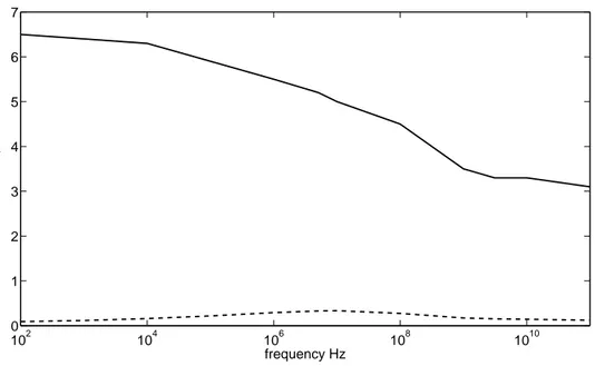
Figure 2.2 gives the ǫ′
and ǫ′′
of the wood cellular material as a func-tion of frequency. The figure was obtained with data from [17]. The parameters were obtained for electric field oriented perpendicularly to the wood tubular cells. It can be seen that the dielectric behavior
of the wood cell wall substance is typical of a polar substance, as ǫ′
decreases with frequency, with a fall at the frequency where ǫ′′
has its peak. This behavior indicates the presence of polar molecules in
wood, but the difference in ǫ′
at lower and high frequencies, due to the dipole polarization, is only of about three units.
Variation with temperature
Temperature influences the relaxation time of the wood molecules, which decreases with rising temperatures [17]. Even so, the effect of temperature on the dielectric properties of wood is rather small when compared to the influence of temperature on the properties of water. This can be seen in Figure 2.3.
102 104 106 108 1010 0 1 2 3 4 5 6 7 frequency Hz ε
Figure 2.2: The ǫ of the wood cell wall substance at the
tempera-ture 20-25 as a function of frequency. Values are for electric field
perpendicular to the wood tubular cells and published by [17].
2.2.4
Permittivity of moist wood
Hydrogen atoms in the water molecule tend to form hydrogen bounds between themselves and with other molecules. When water is added to a solid it forms bounds with the surface molecules of the solid phase. The hydrogen bounds restrict the movement of the water
molecules and decrease its ǫ′
. Wood has a very large internal surface due to its fibrous structure. This high surface area is able to bind large quantities of water. Torgovnikov [17] defines the wood fiber saturation point as the point where all the water in wood cells is bound. Beyond this point all water is kept inside cell cavities by mechanical forces only. For most wood species the mean value generally accepted for the fiber saturation point is equivalent to a mass of water of 30% of the dry mass [17].
The permittivity of bound water varies with the material to which it is bound. The influence of frequency in the permittivity of a mixture with both bound and free water phase is more complex than the influence on the free water molecule described in 2.2.2.
In a material with both free and bound water phases, temperature 30
variations can result either in a decrease or an increase of the total ǫ′
. The increase of ǫ′
with temperature can be explained by the ”re-lease” of the bound water at higher temperatures resulting in a higher amount of free water that becomes able to participate in dipole
po-larization to a larger extent. The decrease of ǫ′
and the release of bound water into free water with raising temperature are two
com-peting phenomena. Jones and Or [19] analyzed measurements of ǫ′
of soil. The authors show that for lower water content, where bound water dominates over free water, an increase in temperature results in an increase in ǫ′
, because more water is free to participate in dipole
polarization. At higher water contents ǫ′
decreases with temperature because the free water phase is dominant. Somewhere in the mid-dle the two phenomena neutralize each other and a variation in the
temperature leaves ǫ′
unchanged.
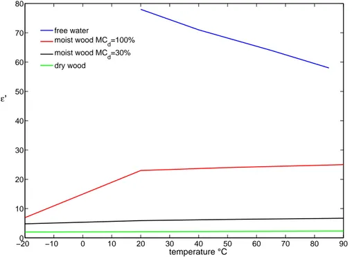
Figure 2.3 shows the ǫ′
of dry wood, moist wood with 30% and 100% of water as a percentage of the dry mass, and of free water
respec-tively, as a function of temperature for a frequency of 108
MHz and a
wood density of 0.6 g·cm−3
. The values used were published by [17]. In Figure 2.3 the complex influence of free and bound water in wood
can be noticed. While the ǫ′
of free water decreases with tempera-ture, the ǫ′
of moist wood increases with temperature. The influence
of temperature on the ǫ′
of dry wood is very small and the influence is larger for higher water contents as the dielectric properties become
determined by those of water. The ǫ′
of water decreases with temper-ature but the ǫ′
of moist wood increases with temperature. This can be explained by the phenomenon described by Jones and Or: that wa-ter is released from the bound state at higher temperatures. In fact, Chudinov and Andreev, cited by Torgovnikov [17], observed that the amount of bound water in wood decreases for higher temperatures. The ǫ′′
of moist wood is higher at lower frequencies were ionic
con-ductivity takes place, but at frequencies above 107
Hz the relaxation
losses are the most important factor. For a frequency of 108
Hz, the ǫ′′
of moist wood increases with water content and temperature. At 108
Hz, 20 and a water content of 100% of the dry mass, the relation
ǫ′′
/ǫ′
of moist wood with 0.6 g· cm−3
−200 −10 0 10 20 30 40 50 60 70 80 90 10 20 30 40 50 60 70 80 temperature °C ε’ free water moist wood MC d=100% moist wood MC d=30% dry wood Figure 2.3: The ǫ′
of free water, oven-dry wood, wood with M Cd=30%
and wood M Cd=100%, for a frequency of 10
8
Hz, and as a function of temperature. Values are for electric field perpendicular to the wood
tubular cells and for a wood density of 0.6 g·cm−3
and published by [17].
2.3
Water content
2.3.1
The relationship between water content and
dielectric properties
In order to relate electromagnetic measurements with the water con-tent, an equation is needed. In this thesis the electromagnetic mea-surements consist of time-domain reflection data. Two methods were used to relate the measurements to water content: use of time-domain
data in a PLS model and calculation of ǫ′
from the wave velocity. As
noted from section 2.2.4 the ǫ′
of moist wood is strongly influenced by the water content and can therefore be used to determine this parameter.
Time-domain reflection data can be related to water content using 32
multivariate data analysis methods such as partial least square regres-sion (PLS). In this case the reflection coefficients at different times are the independent variables. PLS is able to predict one or a set of dependent variables from a large set of independent variables. It com-bines principal components analysis and multiple regression. While principal component analysis finds the orthogonal linear combinations (latent variables) of the dependent variables in order to explain the variance in this set, PLS finds the latent variables that have maxi-mum correlation with the dependent variable set [20]. PLS has been used to relate time-domain RF signal with the water content of woody biomass [7].
The relation between ǫ′
and water content can be established by statis-tical or physical models. An example of a statisstatis-tical equation relating ǫ′
to water content is Topp’s equation derived for prediction of soil water content [15]. This equation has been found to predict water content in soil and other porous materials accurately and is widely used [21, 22, 23]. It is also possible to make use of physically based models, such as mixing models. These models are based on the as-sumption that the dielectric properties of a mixture are a function of the dielectric properties of the individual components of the mixture, their fractional volumes, and on polarization effects dependent on the shape of the components, as expressed in equation (2.9):
ǫ′ m = f ( I X i=1 (ǫ′ i, θi, Dpi)) (2.9) where ǫ′
m is the relative dielectric constant of the mixture, ǫ
′
i is relative
dielectric constant of the component i, θi is the volumetric content of
the component i and Dpi accounts for the particle shape in component
i. Empirical parameters are incorporated into some mixing models in order to improve their performance in practical applications, whereas others have a purely theoretical basis. Theoretical mixing models are valuable for improving our understanding of the dielectric behavior of the mixture [16]. Mixing models have been applied to describe the dielectric behavior of different materials such as soil [24, 25], granular materials [23, 26], snow and ice [27, 28].
2.3.2
Reference water content
The reference method for determining the water content in woody biomass is the standard gravimetric method. This method consists of first weighing a sample of the material, drying the sample in an oven and then weighing the dry material. The weight difference between the wet and dry material is considered to be the mass of water in the sample. This method is fully described in the standard [29].
The application of the reference method requires sampling of the ma-terial whose water content is to be determined. The procedure for sampling woody biomass for water content determination with the standard oven method is described in the standard [30].
2.3.3
Water content definitions
There are different definitions of water content depending on the way in which this parameter is calculated. Water content can be calculated on a volumetric basis. This is called volumetric water content or
volumetric water fraction, θw, and it is calculated according to 2.10:
θw =
Vw
Vt
[m3
· m−3] (2.10)
where Vw is the volume of water and Vt is the total volume. Water
content can also be calculated on a gravimetric basis. In this case it
can be defined as the mass of water, Mw as percentage of the total
mass of the sample, Mt, as shown in equation 2.11 or as a percentage of
the mass of dry matter in the sample, Ms, according to equation 2.12:
M Cw = Mw Mt · 100 [%] (2.11) M Cd = Mw Ms · 100 [%] (2.12)
M Cd is a useful definition when the analysis is related with the
amount of bound water. The amount of bound water in wood de-pends on the amount of dry matter. The generally accepted value for
the maximum amount of bound water in wood M Cd= 30% [17]. To
verify the amount of bound and free water in a sample it is therefore important to express the water content as a percentage of the dry matter.
θw is the most used definition when studying the dielectric behavior
of moist mixtures. ǫ′
m is better explained as a function of the
volu-metric content than as a function of the gravivolu-metric content of the constituents due to bulk density effects. This is shown, for instance, by Hallikainen et al. [31] for ǫ′
m of soil against θw and M Cw.
M Cw is a widely used definition of water content and probably the
one whose value can be perceived most directly. The standard oven method for water content gives results in gravimetric units and in many cases it is not possible to calculate the volumetric content with the same accuracy due to difficulties in volume measurement. It is
possible to calculate θw from M Cw using the relation in 2.13:
θw = M Cw 100 · ρt ρw [%] (2.13)
where ρt is the density of the sample calculated as Mt/Vt and ρw is
the water density.
2.4
Measurement systems
Dielectric properties can be measured accurately using different labo-ratory methods, but not all of them are adequate when measurements outside laboratory conditions are required. Examples of ments outside laboratory conditions are, for instance, the measure-ment of soil or a crop canopy directly in the field and measuremeasure-ments of materials in an industrial line. These applications often require that the materials are measured without touching or destroying them. They also require a set-up that is able to measure in a range of situa-tions that may imply moving the material, measuring a large portion of the material and measurements in different kinds of sample holders. Several microwave and RF systems have been developed to measure water content on-line in materials such as grain, powders, foodstuffs
or mineral ore. A review of these can be found in [6, 32]. However, these methods cannot measure large volumes of material. A material whose measurement demands can be compared with the bulk mea-surement of woody biomass in containers is soil. The meamea-surement of water content in soil in-field is of great importance in fields like agri-culture, hydrology or civil engineering. Therefore several studies have been done within this area. A successfully developed technique has been time domain reflectromety, TDR. TDR makes use of the wave velocity in a transmission line inserted in the soil to determine soil water content and uses the attenuation to determine soil conductiv-ity [33]. TDR probes are limited to measurements of volumes up to 1 dm3
[34]. Ground penetrating radar, GPR, has been used to measure water content in larger areas of soil [35]. Several methods are used in soil water content measurements with GPR. When the depth to a reflector, such as a water table, is known, the travel time to that
reflector can be used to calculate the velocity of the waves in soil. ǫ′
can be calculated and correlated with the average water content in the zone before the reflector. Stoffregen et al. [36] used this method to determine average water content at a soil depth of 1.5 m.
The calibration models and the prediction results can be evaluated and compared by calculating the root mean square error, RMSE, according to equation (2.14): RM SE = v u u t N X n=1 (ymeas − ymod)2 N (2.14)
where N is total the number of samples, ymeas is the measured
pa-rameter and ymod is the parameter calculated with the model. The
RMSE is commonly named root mean square error of the calibration when calculated with samples used to build a model, and root mean square error of prediction when it is calculated with an independent set of samples.
2.4.1
Laboratory-scale system for bulk
measure-ments of woody biomass
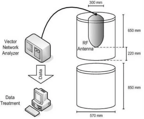
A system for bulk measurements of woody biomass was developed by Nystr¨om [7]. A diagram of this measurement system can be seen in figure 2.4.The system is composed of two linked steel drums, one acting as a sample holder and the other protecting the antenna from the environment. The two drums act as a wave guide with a short circuit at the far end. A network analyzer and a log periodic antenna were used to emit a sweep of frequencies between 310-800 MHz. The RF waves are sent by the antenna, travel through the material and are reflected at the bottom of the sample holder and back to the antenna.
Figure 2.4: Scheme of the laboratory-scale measurement system. The upper drum shield the RF antenna, which is connected to a vector network analyzer. The other drum contains the sample and the two are connected during the measurements.
The reflection coefficient is calibrated with a short-open-offset cali-bration and transformed into the time domain. It is then possible to identify reflection from the surface of the biomass and from the
bottom of the container. The travel time through the sample can be obtained by the difference between the times of the reflections at the bottom and at the biomass surface. The velocity of the RF waves in biomass can be calculated using the travel time and the height of the sample using equation (2.7). A detailed description of the system can be found in [37].
Water content in woody biomass with this system has been predicted using a statistical model built with PLS, obtaining a RMSE of
pre-diction of about M Cw=2.7% [7].
Chapter 3
Contributions of the thesis
In this chapter the contributions of each paper included in this thesis are presented. A r´esum´e of the aim, methods, results and conclusions are also presented. The aim is to give a comprehensive view of the work done within each of the three papers.The following main contributions of the thesis can be listed:
- Evaluation of the influence of temperature on the ǫ′
m and water
content measurements of woody biomass within the 1-62 range
(Paper I ).
- Analysis of the behavior of the ǫ′
m of woody biomass and
develop-ment of a semi-physical model that is able to describe this behavior (Paper II ).
- Test the use of ǫ′
m to predict water content in woody biomass (Paper
II ).
- Full-scale measurement of ǫ′
m of woody biomass (Paper III ).
3.1
Influence of temperature in the
ǫ
′m
of
woody biomass
The variation of ǫ′with temperature in water, wood and moist wood was discussed in Chapter 2. The influence of temperature in a mixture with both bound and free water phases is complex and difficult to
predict because it depends on the water content and on the degree
of binding. Therefore studying the influence of temperature in ǫ′
m of
woody biomass was of interest.
In Paper I the study of the influence of temperature in dielectric measurements of water content in woody biomass is presented. The influence of temperature was investigated by performing a total of sixty measurements of six different biomass samples at different
tem-peratures. The M Cw of the samples varied between 31% and 63%,
which correspondent to a M Cd between 46 and 167%. Measurements
were made with temperatures varying from 1 to 62 . The following
procedures were used in the analysis of the results:
- Study of the travel time and attenuation for different sample tem-peratures;
- Principal component analysis of the data;
- Evaluation of the prediction ability for an independent validation set with varying temperatures using a model built with samples measured at room-temperature only.
3.1.1
Results and discussion
The results presented in Paper I show that variations in attenuation and travel time of the signal can occur for the same sample, but it was not possible to correlate these variations with the temperature. In the multivariate data analysis it was noticed that it is not possible to identify temperature in the score plot with the principal compo-nents that describe the data set.
The validation with independent test sets show that using samples with different temperatures does not seem to affect the prediction ability of a model calibrated with samples at room-temperature.
In Figure 3.1, ǫ′
m calculated from the travel time of the samples is
presented as a function of temperature for the six samples used in the
study. It can be noticed that for samples with same water content, ǫ′
m
can vary for different sample temperatures. However this variation is rather small and it is not possible to detect a trend in these variation related with the sample temperature. In Figure 2.3 it is possible to
see that larger variations of ǫ′
with temperature occur for wood with
larger water content, but that even for wood with M Cd= 100% this
variation is minimal after 20 . Between 0 and 20 the ǫ
′
m of moist
wood increases significantly. The variation in ǫm of woody biomass
presented in Figure 3.1 cannot be related with the behavior of ǫ′
m of
moist wood at different temperature. These variations are introduced by other parameters, such as measurement system or measurement procedure. 0 10 20 30 40 50 60 70 3 3.5 4 4.5 5 5.5 6 6.5 7 temperature ° C ε’ m MC d= 46% MC d= 76% MC d= 84% MC d= 107% MC d= 128% MC d= 167% Figure 3.1: The ǫ′
m of woody biomass as a function of temperature
for samples with six different water contents.
3.2
Dielectric Mixing models
In Paper II the behavior of ǫ′
m of woody biomass is studied. The
aim was to study if the ǫ′
m, calculated from the wave velocity in the
basis and verify that such a model can be used to predict water content in the mixture.
Understand the relation between dielectric measurements and water content is important to the development of measurement systems.
A calibration model based on ǫ′
m could be applied in systems with
different equipment, set-up or different sample sizes.
The dielectric behavior of biomass was studied using dielectric mixing
models. These models make use of the volumetric fractions, ǫ′
, and
the geometry of each constituent of the mixture to determine the ǫ′
m.
ǫ′
m is better explained as a function of the volumetric content than
as function of the gravimetric content of the constituents due to bulk density effects. This can be seen in Figure 3.2, which shows the
experimental ǫ′
m data for woody biomass plotted as a function of the
three water content definitions presented in section (2.3.3): θw, M Cw
and M Cd. It can be noticed that the variation of ǫ
′
m for the same water
content is smaller when θw is used. This is because samples with the
same M Cw and different bulk densities can have significantly different
ǫ′
m while samples with same θw and different bulk densities result in
approximately the same value of ǫ′
m.
The relation between ǫ′
m and θw for woody biomass obtained with
experimental data shows a unique sort of behavior: within a range of
θw between 0.07 and 0.27 ǫ′m of woody biomass varies between 2.5 and
7.5, within the same range the ǫ′
m of soil can vary between 2.5 and
20 [38], while in corn, for a θw range between 0 and 0.13, ǫ
′
m varies
between 2 and 7 [23].
Woody biomass can be considered a mixture of air, water and wood. Wood has a very large surface area, which can bind large amounts of water. This introduces a unique and varied dielectric constant-water content behavior [18]. This was the object of study in Paper II, where a semi-physical model, the power law model and two physical models, the Maxwell Garnett (MG) and the Polder van Santen (PS) models, were used. In these models woody biomass was considered to be a four-phase mixture of air, wood cellular material, bound and free water. Air was considered to be the host. Different geometries were studied in order to obtain the best fit of the data. Finally the model which most successfully described the experimental data was
used for determining θw with an independent validation set.
0 0.2 0.4 2 3 4 5 6 7 8 θ w [m 3.m−3] ε’ m 20 40 60 80 2 3 4 5 6 7 8 MC w [%] ε’ m 0 100 200 2 3 4 5 6 7 8 MC d [%] ε’ m Figure 3.2: The ǫ′
m of woody biomass as a function of different water
content definitions: θw, M Cw and M Cd. It can be noticed that the
dispersion is smaller when θw is used.
3.2.1
Results and discussion
It was found that the MG model was able to describe the behavior of ǫ′
m of woody biomass. This model was obtained using disc-like
geom-etry for the bound water inclusions and oblate ellipsoidal geomgeom-etry for the free water inclusions. These geometries resulted in the best fit of the experimental data. It was found that the influence of the geometry of wood cellular material inclusions can be neglected, as the θ and ǫ′
of this phase are rather small. Although the MG model was able to explain satisfactorily the trend in the experimental data, it is difficult to base the results of the best fitting geometries on the structure of the biomass constituents. In this manner the resultant model is a semi-physical model, as some parameters were obtained by fitting and lack justification in physical characteristics.
predic-tion of volumetric water content results in a RMSE of 0.029 m3
·m−3. This result is on the same order as prediction error results found in soil water content measurements [34]. However, when using the mean density of the biomass samples to convert the error to gravi-metric units, according to equation (2.13), a RMSE of prediction of
M Cw=8.9% is obtained. This is a larger error than using multivariate
data analysis to predict water content, as was done in Paper I, where
the highest RMSE of prediction obtained was M Cw=2.6%.
3.3
Full-scale measurements
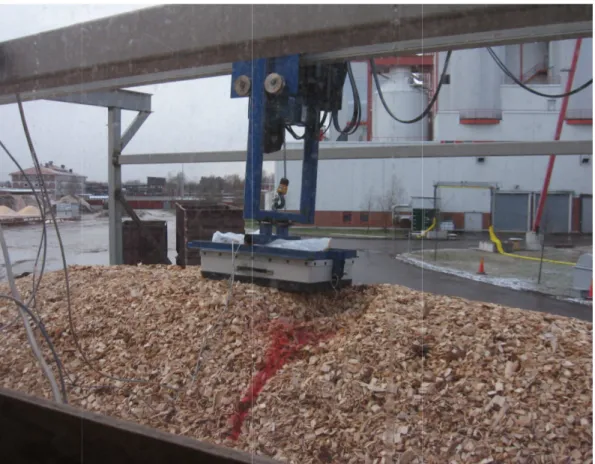
Paper III describes results from full-scale RF measurements of woody biomass, which entails that measurements were made directly in the containers where the biomass is transported. Figure 3.3 shows a pic-ture of the GPR antenna placed on the surface of the biomass. The set-up that holds the antenna and moves it along the biomass surface is also visible. A detailed description of the set-up can be found in [8].
The biomass deliveries measured had a volume of about 100 m3
while in the laboratory-scale method the samples had a volume of about 0.1 m3
. The full-scale system measures the entire depth of material in a container and the reference value obtained from the standard gravi-metric oven method is not representative of volume measured with RF. For this reason it was important to use the laboratory-scale
mea-surements as a comparison. In Paper II ǫ′
m for the laboratory-scale
measurements was calculated from the velocity of the waves in the sample and its behavior was explained based on a theoretical model. In Paper III, ǫ′
m is calculated in the same manner and compared with
results from laboratory-scale measurements.
It was shown in section (3.2) that ǫ′
m was better correlated with θw
than with gravimetric water content. Nevertheless, when studying
full-scale results the correlation between ǫ′
m and θw was worse than
the one between ǫ′
m and M Cw. This is probably due to the estimation
of the total volume of the material, which is used to calculate θw
from the gravimetric reference value, as seen in equation 2.13. This estimation is not very accurate and might introduce random errors in
Figure 3.3: Picture of the full-scale measurements. The GPR antenna is placed on the surface of woodchips inside a transport container at a combined heat and power plant.
the conversion of the reference value from gravimetric to volumetric
water content. For this reason the water content definition M Cw was
used in this study. In Paper III, ǫ′
m of the laboratory-scale measurements was plotted as
a function of M Cw and a fitting curve was obtained. Analyzing the
results was done according to the following:
- The relation between ǫ′
m and M Cw for the laboratory-scale
mea-surements was studied;
- The relation between ǫ′
m and M Cw for the full-scale was studied
and compared with the same relation for the laboratory-scale mea-surements;
- Calibration equations for relation ǫ′
m-M Cw for both laboratory and
full-scale measurements were obtained and evaluated;
by taking samples from different parts of the biomass tipped on the ground.
3.3.1
Results and discussion
The relation between ǫ′
m and M Cw in the full-scale measurements
shows agreement with the same relation in laboratory-scale measure-ments. Both fitting curves follow the same trend but the dispersion is larger for full-scale measurements. This result indicates that a calibration model obtained with accurate reference values with the laboratory-scale measurements could be used to predict the water content in the full-scale measurements.
Multiple measurements in a delivery of biomass tipped on the ground
gave a maximum variation of 11% in M Cw and a maximum standard
deviation of 5.6.
The RMSE for the calibration curves was 4.5% for the laboratory-scale calibration curve and 7.3% for the full-laboratory-scale. The larger error in the full-scale situation might be due to the large depth of material and the open-air setup. This could also be due to inaccuracy in the full-scale reference value which would mean a smaller actual error.
The RMSE value obtained with the fitting curve between ǫ′
m and
M Cw for full-scale measurements is rather large. Different methods,
such as PLS, should be tested to investigate if it is possible to obtain better results with the woody biomass bulk measurement system.
Chapter 4
Conclusions
The conclusions are stated according to the four questions defined in the beginning of the thesis:
Concerning the influence of temperature on ǫ′
m of woody biomass,
it was found that it is not possible to associate variations in ǫ′
m with
temperature variations. It was also shown that temperature variations
within 1 and 62did not influence the water content prediction error
when using a PLS model calibrated only with samples measured at
about 20 .
Concerning the behavior of ǫ′
m of woody biomass, this could be
ex-plained using the MG model, by assuming that woody biomass is an isotropic mixture of air, wood cellular material, free and bound water. However, the depolarization factors, used in the model to account for the geometry of the inclusions, were obtained by statistical fitting and results were found to be difficult to base on physical biomass characteristics.
The prediction of water content with the MG model which was able to
describe the experimental data, obtained a RMSE of 0.029 m3
·m−3. This error is larger than the prediction error obtained when PLS is used as a calibration model.
In the full-scale measurements an empirical model relating ǫ′
m with
the M Cw obtained resulted in a RMSE of calibration of 7.3%. This
value is obtained when using values from the oven reference method,
which might not be accurate. The relation between ǫ′
m of biomass
and M Cw followed the same trend in full-scale measurements as in
Chapter 5
Future work
This thesis concentrated on the study of the dielectric constant of woody biomass and its use in water content prediction. Although this study is important to understanding the dielectric behavior of woody biomass, the use of the dielectric constant to predict water content resulted in larger prediction errors than when using PLS mod-els. Further analysis of the full-scale measurements has to be carried out, namely using PLS methods, to verify if it is possible to obtained smaller prediction errors.
PLS models account for the attenuation in the material since the reflection coefficient data in time-domain is used. It is possible that PLS models give better water content prediction due to this fact,
which raises the interest in studying the ǫ′′
of woody biomass.
Another challenge is the possibility of measuring other biomass char-acteristics using the dielectric properties at radio frequencies. An ex-ample of an interesting parameter when woody biomass is used as a fuel, is the ash content, in other words the nonvolatile inorganic mat-ter which remains afmat-ter the combustion. Demat-termining the inorganic content in biomass can be related with the electrical conductivity. The measurement of electrical conductivity with RF has also been a successfully achieved using TDR in soils.
Bibliography
[1] Biomass action plan. European Commission, 2005.
[2] Energy in sweden, figures and facts. Swedish Energy Agency, 2007.
[3] J Nystr¨om and E Dahlquist. Methods for determination of mois-ture content in woodchips for power plants - a review. Fuel, 83(7-8):773 – 779, 2004.
[4] L Axrup, K Markides, and T Nilsson. Using miniature diode ar-ray NIR spectrometers for analyzing woodchips and bark samples in motion. Journal of Chemometrics, 14:561–572, 2000.
[5] Barale P, Fong C, Green M, Luft P, Mcinturff A, Reimer J, and Yahnke M. The use of a permanent magnet for water content measurements of wood chips. IEEE transactions on applied su-perconductivity, 12(1):975–978, 2002.
[6] S Okamura. Microwave technology for moisture measurement. Subsurface Sensing Technologies and Applications, 1(2):205–227, 2000.
[7] J Nystr¨om. Rapid measurements of the moisture content in bio-fuel. PhD thesis, M¨alardalen Univeristy, 2006.
[8] A Paz, J Nystr¨om, and E Dahlquist. Water content measurement of biofuel with RF directly in trailers truck containers. Technical report, V¨armeforsk, in manuscript.
[9] L Chen, C Ong, C Neo, V V Varadan, and V K Varadan. Microwave electronics, measurement and materials characteri-zation. Wiley, 2004.
[10] E Nyfors and P Vainikainen. Industrial Microwave Sensors. Artech House, 1994.
[11] A Hippel. Dielectric materials and applications: papers by
twenty-two contributors. Technology Press of M.I.T and Wiley, New York, 1954.
[12] F Ulaby. Fundamentals of applied electromagnetics. Pearson Prentice Hall, 5 edition, 2007.
[13] J Hasted. Aquous Dielectrics. Chapman and Hall, 1973.
[14] D Cheng. Field and wave electromagnetics. Addison Wesley, 1989.
[15] G Topp, J Davis, and A Annan. Electromagnetic determination of soil water content: measurements in coaxial transmission lines. Water Resources Research, 16(3):574 – 582, 1980.
[16] D Robinson, S Jones, J Wraith, D Or, and S Friedman. A review of advances in dielectric and electrical conductivity measurement in soils using time domain reflectometry. Vadose Zone Journal, 2(4):444–475, 2003.
[17] G Torgovnikov. Dielectric properties of wood and wood based materials. Springer-Verlag, 1992.
[18] U Kaatze. Electromagnetic wave interaction with water and
aqueous solutions. In Electromagnetic Aquametry. Springer,
2005.
[19] S Jones and D Or. Modeled effects on permittivity measurements of water content in high surface area porous media. Physica B: Condensed Matter, 338(1-4):284–290, 2003.
[20] H Abdi. Partial least squares (PLS) regression. In Encyclopedia of Social Sciences Research Methods. Sage, 2003.
[21] C Dirksen and S Dasberg. Improved calibration of time domain reflectometry soil water content measurements. Soil Science So-ciety of America Journal, 57(3):660 – 667, 1993.
[22] A Turesson. Water content and porosity estimated from ground-penetrating radar and resistivity. Journal of Applied Geophysics, 58(2):99–111, 2006.
[23] M Vallone, A Cataldo, and L Tarricone. Water content estima-tion in granular materials by time domain reflectometry: A key-note on agro-food applications. In IEEE Instrumentation and Measurement Technology Conference, pages 1091–5281, Warsaw, Poland, 2007.
[24] H Gong, Y Shao, J Liu, Q Hu, and W Tian. Improved model for dielectric behavior of moist saline soil. In Proceedings of the Inter-national Society for Optical Engineering, volume 6787, Wuhan, China, 2007.
[25] M Dobson, F Ulaby, M Hallikainen, and M El-Rayes. Microwave dielectric behaviour of wet soil. II dielectric mixing models. IEEE Trans. Geosci. Remote Sens. (USA), GE-23(1):35 – 46, 1985. [26] M Hilhorst, C Dirksen, F Kampers, and R Feddes. New dielectric
mixture equation for porous materials based on depolarization factors. Soil Science Society of America Journal, 64(5):1581 – 1587, 2000.
[27] M Hallikainen, F Ulaby, and M Aderlrazik. The dielectric be-haviour of snow in the 3 to 37 GHz range. In IGARSS ’84. Re-mote Sensing - From Research Towards Operational Use, pages 169 – 174, Strasbourg, France, 1984.
[28] A Sihvola. Electromagnetic mixing formulas and applications. The Intitution of Electrical Engineers, 1999.
[29] SS187170. Biofuels and peat- determination of total moisture. Swedish Standard Institution, 1998.
[30] SS187113. Biofuels and peat - sampling. Swedish Standard In-stitution, 1999.
[31] M Hallikainen, F Ulaby, M Dobson, M El-Rayes, and L Wu. Microwave dielectric behavior of wet soil. I empirical models and
experimental observations. IEEE Transactions on Geoscience and Remote Sensing, GE-23(1):25 – 34, 1985.
[32] K Lawrence and S Nelson. Radiofrequency sensing of mois-ture content in cereal grains. In Sensors Update, pages 377–391. Wiley-VCH, 2000.
[33] P Ferre and G Topp. Time-domain reflectometry techniques for soil water content and electrical conductivity measurements. In Sensors Update, pages 277–300. Wiley-VCH, 2000.
[34] J Huisman, C Sperl, W Bouten, and J Verstraten. Soil water content measurements at different scales: accuracy of time do-main reflectometry and ground-penetrating radar. Journal of Hydrology, 245(1-4):48–58, 2001.
[35] J Huisman, S Hubbard, J Redman, and A Annan. Measuring Soil Water Content with Ground Penetrating Radar: A Review. Vadose Zone J, 2(4):476–491, 2003.
[36] H Stoffregen, T Zenker, and G Wessolek. Accuracy of soil water content measurements using ground penetrating radar: compar-ison of ground penetrating radar and lysimeter data. Journal of Hydrology, 267(3-4):201–206, 2002.
[37] J Nystr¨om and B Franzon. Radio frequency system for mea-suring characteristics of biofuels. In Proceedings of the IEEE Instrumentation and Measurement Technology Conference, Ot-tawa, Ontario, Canada, 2005.
[38] N Peplinski, F Ulaby, and M Dobson. Dielectric properties of soils in the 0.3-1.3GHz range. IEEE Transactions on Geoscience and Remote Sensing, 33(3):803–807, 1995.
![Figure 2.1: The ǫ of free water at 0, 20 and 60 as a function of frequency. The complex permittivity was calculated using the Debye equation with parameter values published by [18].](https://thumb-eu.123doks.com/thumbv2/5dokorg/4823534.129953/30.892.206.693.142.517/figure-function-frequency-permittivity-calculated-equation-parameter-published.webp)