V¨
aster˚
as, Sweden
Thesis for the degree of Master of Science in Engineering - Robotics,
30.0 credits
FPGA acceleration of superpixel
segmentation
Student:
Magnus ¨
Ostgren
M¨
alardalen University, V¨
aster˚
as, Sweden
Student ID: mon15008
Supervisor:
Carl Ahlberg
M¨
alardalen University, V¨
aster˚
as, Sweden
Examiner:
Mikael Ekstr¨
om
M¨
alardalen University, V¨
aster˚
as, Sweden
is split into segments referred to as superpixels. Then running the main algorithm on these su-perpixels reduces the number of data points processed in comparison to running the algorithm on pixels directly, while still keeping much of the same information. In this thesis, the possibility to run superpixel segmentation on an FPGA is researched. This has resulted in the development of a modified version of the algorithm SLIC, Simple Linear Iterative Clustering. An FPGA imple-mentation of this algorithm has then been built in VHDL, it is designed as a pipeline, unrolling the iterations of SLIC. The designed algorithm shows a lot of potential and runs on real hardware, but more work is required to make the implementation more robust, and remove some visual artefacts.
AXI Advanced eXtensible Interface BSDS Berkeley Segmentation Data Set CPA Centre Perspective Architecture CPU Central Processing Unit
CRS Contour Relaxed Superpixels
DRAM Dynamic Random Access Memory DSP Digital Signal Processor
EOL End Of Line
ERGC Eikonal Region Growing Clustering ERS Entropy Rate Superpixels
ETPS Extended Topology Preserving Segmentation FA Full Adder
FF Flip-Flop
FPGA Field Programmable Gate Array FPS Frames Per Second
FP-SLIC Fully Pipelined - Simple Linear Iterative Clustering GPU Graphics Processing Unit
HDL Hardware Description Language HLS High-level Synthesis
IoT Internet of Things IP Intellectual Property LUT Lookup Table
MDH M¨alardalens H¨ogskola M¨alardalen University MUX Multiplexer
PPA Pixel Perspective Architecture RAM Random Access Memory
SEEDS uperpixels Extracted via Energy-Driven Sampling SLIC Simple Linear Iterative Clustering
S-SLIC Subsampled - Simple Linear Iterative Clustering SNIC Simple Non-Iterative Clustering
SoC System on Chip SOF Start Of Frame SP superpixel
1.1 Problem formulation . . . 1
1.1.1 Research questions . . . 1
1.1.2 Limitations . . . 1
2 Background 2 2.1 Superpixels . . . 2
2.2 Evaluation of superpixel segmentation . . . 3
2.3 FPGA . . . 3
2.4 Video over AXI4-Stream . . . 4
2.5 PYNQ . . . 5
3 Related works 5 3.1 S-SLIC ASIC . . . 5
3.2 SEEDS on FPGA . . . 6
3.3 Evaluation and comparison of state-of-the-art superpixel algorithms . . . 6
4 Method 6 4.1 Methodology . . . 7
5 Implementation 7 5.1 High-level proof of concept . . . 7
5.2 Low-level design and simulation . . . 8
5.2.1 Delays . . . 9
5.2.2 Superpixel stores . . . 9
5.2.3 Superpixel update units . . . 10
5.2.4 Initialisation and labelling . . . 11
5.2.5 Simulation . . . 11
5.3 FPGA implementation and testing . . . 12
6 Results 12 6.1 High-level implementation . . . 12
6.2 Simulation of low-level implementation . . . 13
6.3 FPGA implementation . . . 15
7 Discussion 15 7.1 High-level implementation results . . . 16
7.2 Low-level implementation results . . . 16
7.3 Research questions . . . 18
8 Conclusion 18
References 21
1
Introduction
Embedded systems for real-time computer vision applications is a growing research area with use cases in everything from small IoT devices to self driving cars. One thing that is true for most of these applications is the need to process the incoming images fast enough to utilise their information while it is relevant. How fast that is, of course, depends on the application in question, but for robots and other autonomous systems faster is often better.
The combination of sophisticated computer vision algorithms, high resolution images and sig-nificant speed requirements is not compatible with the computing power of a microcontroller or other embedded CPUs. One solution to this is the use of a heterogeneous computing platform, supplementing the CPU with a highly parallel co-processor, like a graphic processing unit(GPU) or a specialised accelerator on a field programmable gate array(FPGA). Another approach is to first process the images in some way to reduce the amount of data that the application algorithm has to process. This thesis will look at a combination of these two approaches; FPGA acceleration of a general purpose preprocessing algorithm to reduce the computational load of computer vision algorithms. This preprocessing will be based on superpixel segmentation, introduced by Ren and Malik in the paper Learning a classification model for segmentation [1].
The main idea of superpixel segmentation is that the image is split into segments of uniform size and shape, that are internally consistent in colour. Application algorithms can then work on these superpixels instead of normal pixels, significantly reducing the number of data points processed.
1.1
Problem formulation
This thesis aims to create a superpixel segmentation accelerator on an FPGA. For superpixel segmentation to be a viable preprocessing step in an embedded system, computing the superpixels and then running the application algorithm, must be faster than running the application algorithm on the raw image. To reduce latency and keep up with real-time requirements, this implementation is limited to resources on the FPGA, i.e. it should not require external components like DRAM. During this thesis, no hard constraints are set on the size of the FPGA implementation, but the resource usage should be kept in mind.
The target device that the implementation should run on is the Zynq-7020 from Xilinx.
1.1.1 Research questions
To accomplish the goal set in the Problem formulation, the following research questions have been stated to lead the way to a successful and state-of-the-art FPGA implementation of superpixel segmentation.
Q1. What algorithm, or algorithms, do other research point to as state-of-the-art in superpixel segmentation?
Q2. Can the superpixel segmentation algorithms from Q1 be implemented on an FPGA? Q3. What are the advantages of implementing superpixel segmentation on an FPGA? Q4. What are the limitations of superpixel segmentation implemented on an FPGA?
1.1.2 Limitations
The time limitation of 20 weeks makes it highly improbable that multiple algorithms will be implemented on an FPGA, to be compared. This means that even if multiple algorithms are found to be suitable for FPGA implementation during the research phase, only one of them will be developed to an FPGA implementation. This can impact the answer to the research questions Q3 and Q4, as different algorithms will have different properties and it is not entirely certain that the optimal solution will be developed.
Another limitation is that this thesis will be able to give a positive answer to the research question Q2, but not a true negative one, only that this work might have been unable to create an FPGA implementation, and in that case, why not.
2
Background
In this section the concepts utilised in this thesis is introduced and briefly explained. These are superpixel segmentation and relevant algorithms for it, as well as a short introduction to FPGAs and development of digital systems for signal processing.
2.1
Superpixels
As stated by Ren and Malik [1], the pixels of an image are not natural entities and the high resolution of modern cameras means that many pixels will carry the same or very similar informa-tion as their neighbours, making them redundant. This is even more true now than it was 2003, when their paper was published, thus making image processing algorithms that compare pixels, like image segmentation, unnecessarily computationally expensive. Their solution to this was to split the segmentation into two steps, first over-dividing the image into small segments that better correspond to natural entities of objects in the image, refered to as superpixels, then building seg-ments from these superpixels. Others have shown that superpixel segmentation can be a powerful preprocessing step for more than image segmentation, for example Miyama uses it to increase the speed of stereo matching [2], and Gu et al. have shown that it can reduce the execution time of some classification problems [3].
One well used algorithm that in a fast and efficient way generates superpixels of good quality is Simple Linear Iterative Clustering, SLIC, developed by Achanta et al. [4]. It is based on K-means clustering and iteratively redefines pixel clusters to minimise the pixel to cluster centre distance. Where cluster centres are originally placed on a uniform grid and distances are measured as a weighted sum of the spatial and colour distance, i.e. the euclidean distances in the XY plane and the CIELAB colour space [5]. This distance, D, is calculated as D = Dc+mS · Ds, where Dc is
the colour distance, Ds is the spatial distance, m is the so called compactness factor, and S is the
grid spacing. m is a coefficient provided by the user and S is calcualted as S =
q
Np
K, where Npis the number of pixels in the image and K is the expected number of superpixels. For every centre, the pixels in an area two times the size of the grid spacing around that centre are checked to see if they are closer to that centre than to their current cluster centre. SLIC can either iterate for a specified amount of iterations or until some criterion like a minimum number of pixels moved between clusters are reached.
Another algorithm that can be considered state-of-the-art, is Simple Non-Iterative Clustering, SNIC [6]; it is an improved algorithm from the research group that developed SLIC. In SNIC, pixels are added to clusters, and in the same way as SLIC it starts with cluster centres on a uniform grid. After a pixel is added to a cluster that cluster centre is updated to the weighted mean of its current position and the new pixel, equaling the mean of all pixels added to the cluster. Then all of the new pixel’s neighbours, that do not already belong to a cluster are pushed on a priority queue with priority based on the distance to the current cluster centre. Distance is calculated in the same way as in SLIC, and smaller distance implies a higher priority. Then the highest priority pixel is popped from the queue, and if it does not already belong to a cluster, it is added to the cluster that put it on the queue. This cycle of reading a pixel and a cluster ID from the priority queue, assigning the pixel to the cluster, and then adding the pixels neighbours and the read cluster ID to the queue, continues until all the pixels in the image are added to clusters. Compared to SLIC, SNIC calculates fewer distances, uses less memory, and does not execute iteratively to find a solution, but pixels are visited in a random pattern, and the complex data structure of a priority queue is required.
SEEDS, Superpixels Extracted via Energy-Driven Sampling developed by Van den Bergh et al. [7] is another algorithm for superpixel segmentation. It initially divides all pixels into superpixel clusters by forming a grid of perfect squares. Pixels are then exchanged between clusters at the borders to maximise an energy function using a hill climbing optimisation scheme. An energy function is a function that expresses the total energy of a system, in SEEDS the energy of a cluster is normally expressed as some function of the similarity of the pixels in the cluster. In a similar way as SLIC, this algorithm iterates until a stop condition is met. That can either be a variable or a fixed number of iterations. The algorithm can be stopped at any iteration and still give a
valid output. Segmentation quality improves with the number of iterations, but compared to an algorithm like SNIC, that needs to run from start to end to output a superpixel segmentation, SEEDS can be aborted to meet a timing deadline and still output superpixels.
Watershed segmentation is a class of segmentation algorithms that, unlike the previous three algorithms, is not defined as clustering of pixels. These algorithms instead locate the borders between segments. The image is transformed to greyscale and then treated as a topographic map. The ridges in that map are then the borders between segments. A fast algorithm to find segments and borders is seeded watershed, proposed by Meyer [8]. It works by growing clusters out from seed points and labelling pixels that neighbour pixels from more than one cluster as border pixels. Clusters are grown in a way similar to SNIC using a priority queue. This is a fast way of segmenting an image, but it does not yield segments of similar size and shape, which is a crucial aspect to using them as superpixels. To solve this, Neubert and Protzel propose the Compact Watershed algorithm [9]. The distance metric used when growing the clusters now also takes the spatial distance to the seed point into account, making the segments much more uniform in both size and shape. In this form proposed by Neubert and Protzel, Compact Watershed seems almost indistinguishable from SNIC.
2.2
Evaluation of superpixel segmentation
In the papers that introduces the superpixel segmentation algorithms presented above, the two most used metrics for comparing and evaluating the quality of superpixel segmentation is boundary recall and under-segmentation error. These metrics are are also the ones used in the standardised evaluation scheme for superpixel segmentation intriduced by Neubert und Protzel [10]. Boundary recall is a measure of how well the edges between the segments coincide with borders in a ground truth, it is calculated as the fraction of how many border pixels in the ground truth that match up to a border pixel in the segementation and the total number of border pixels in the ground truth. Under-segmentation error is a measure of how much a segment leaks outside of the corresponding area in the ground truth. This can be calculated in a couple of different ways, but the method proposed by Neubert and Protzel is to calculate the size of the difference set and and the overlap for every ground truth segement and superpixel pair, add up the smallest of these values from every pair, and then divide with the total number of pairs to get the average. To run these kinds of ground truth-based tests, a dataset of segmented images is required. The datasets that keeps coming up in the papers on superpixels are versions of the Berkeley Segmentation Data Set, BSDS300 [11] and BSDS500 [12]. The original BSDS300 contain 300 images, and the continuation, BSDS500, is extended with 200 images. All of the images in the data sets have multiple ground truths from manual segmentation by humans, on average five different segmentations are available per image.
2.3
FPGA
According to A Practical Introduction to Hardware/Software Codesign [13]
”A Field Programmable gate Array (FPGA) is a hardware circuit that can be reconfigured to a user-specified netlist of digital gates. The program for an FPGA is a ‘bitstream’, and it is used to configure the netlist topology. Writing ‘software’ for an FPGA really looks like hardware develop-ment – even though it is software.” This dualism of FPGAs, being a fixed piece of hardware, but emulating other digital circuits on a gate and register level, using a software configuration, makes them very flexible as computation devices. FPGAs can be configured to behave like specialised hardware implementing a specific algorithm without the hard constraints of fixed devices like a processor, where data path, memory width, pipeline depth and other aspects are set in stone. To achieve this behaviour FPGAs are constructed from what is called configurable logic blocks1. These
logic blocks contain small circuits called logic cells that use programmable lookup tables, LUTs, to implement any logic gate and which output can be either asynchronous or clock synchronised using a D flip-flop. The logic blocks are then connected using a programmable interconnect fabric. A high level overview of both this kind of logic cell and programmable interconnect can be seen in Figure 1. To supplement the abilities of the logic blocks, modern FPGAs also contain blocks
with fixed functions. These are normally circuits like memory, block RAM, or blocks implement-ing often used mathematical operations like addition or multiplication, DSP blocks. A real world example of this type of FPGA architecture can be seen in chapter three of the iCE40 UltraPlus data sheet [14] from Lattice Semiconductor.
LUT LUT FA DFF A B C D CLK OUT
(a) A simplified example of a logic cell. Containing two lookup tables, a full adder, a flip-flop and a few multiplexers.
Interconnect fabric IO blocks
Logic blocks
(b) A simplified example of the in-ternal structures of an FPGA. Logic blocks are connected together and to IO blocks using switch matrices in the interconnect fabric.
Figure 1: The main building blocks of an FPGA are configurable logic blocks, they are made up of small logic cells, figure a show an example of such a logic cell. Their functions are set by configuring the lookup tables and multiplexers, they are then combined into more complex circuits using the programmable interconnect fabric that can be seen in figure b.
To utilise an FPGA in an embedded system, they can be paired with a CPU to handle sequential, more high level tasks, leaving the FPGA with tasks it is better suited for, parallel IO or specialised computations. This trend has led to the development of SoCs(System on a Chip) that combines an FPGA with one or more CPUs on the same semiconductor die. Ahlberg et al. [15] describe a custom embedded system for stereo vision based on such a SoC, the Zynq from Xilinx. They use the FPGA to interface with two cameras and implement multiple image processing algorithms, for example, stereo matching and Harris feature extraction. This is a good example of how an FPGA can be utilised to implement a pipeline of both data acquisition and computation.
2.4
Video over AXI4-Stream
Advanced eXtensible Interface(AXI) stream is an interface and protocol defined in the fourth Advance Microcontroller Bus Architecture(AMBA) specification from ARM for streaming data transfers [16]. In its simplest form, a bit parallel payload is transferred from a master to a slave on a rising clock edge, with a valid/ready handshake for synchronisation. The slave indicates that it is ready to receive data by pulling the flag tready high and the master indicates that it is sending data by pulling the tvalid high. Both of these flags needs to be high for a transfer to take place. The specification also defines a few more signals for more advanced use cases, like defining the end of multi payload packets with tlast, specifying stream ID using tid if multiple streams are combined over the same interface, or something application specific using the tuser lines.
For digital signal processing on FPGAs, this is a fitting protocol for moving data between different parts of the processing pipeline. For image processing, Xilinx defines a subset of the AXI4-Stream protocol for streaming video [17]. The size of the payload, tdata, is sized to hold one pixel,tuser is one bit wide and indicates the first pixel of a frame, and tlast is used to indicate the last pixel of a row. In this use tuser and tlast are also called start of frame, SOF, and end of line, EOL. An example of an AXI stream transfer following this version of the protocol can be seen in Figure 2.
clk 0 1 2 3 4 5 6 7 8 9 10 11 12 tdata A1 A2 A3 A4 A5 A6 B1 B2 B3 tvalid tready tuser tlast
Figure 2: Example of 3x2 pixel video frames, A and B, transferred over an AXI4-Stream. Note that only half of B is transferred.
2.5
PYNQ
PYNQ [18], Python Productivity for Zynq, is an open-source project from Xilinx. As the name suggests, it is a Python framework for Xilinx line of processor and FPGA SoCs, Zynq.
The main idea is that it should be a tool for more straightforward interaction with FPGA designs, expressing the circuits implemented on the FPGA as objects in Python. Compared to the traditional way of working with Zynq devices, where software is written in C, either as a bare metal application, a project specific Linux driver, or a Linux user-space application using more general drivers from Xilinx; Python can lead to faster development.
Under the hood, it is still C code running on Linux. However, PYNQ can use system information exported from Xilinx Vivado to load appropriate drivers; and memory mapped IO, and other
hardware registers are exposed to the Python environment as high-level objects, like Numpy2
arrays. This makes PYNQ well suited for rapid prototyping, as the higher abstraction level of Python is less error prone and leads to a quicker development cycle than what probably would be possible in developing the equivalent software interface in C.
3
Related works
In this section, relevant research in the area of implementing superpixel segmentation on an FPGA, is presented.
3.1
S-SLIC ASIC
Hong et al. [19] have designed an ASIC implementation for a version of SLIC that they call S-SLIC, Subsampled-SLIC. This version of SLIC iterates over the pixels in the image instead of the clusters, and for every accessed pixel, it compares the distance of the pixel to the nine spatially closest cluster centres to determine which cluster the pixel belongs to. To differentiate, the authors call this style of algorithm a pixel perspective architecture, PPA, and the original SLIC a centre perspective architecture, CPA. When comparing the memory usage and amount of calculations per update step between their PPA using 9 centres per pixel and the generic CPA SLIC that uses 2S × 2S pixels per centre, they find that the PPA uses about 2.25 times the amount of calculations but only a third as many reads from memory. This is because with the PPA each pixel is only read once per iteration, but used in nine distance calculations, and with CPA each pixel is on average used in four distance calculations per iteration, but read from memory for each of those times.
The subsampling part of the name indicates that S-SLIC uses only a selection of pixels from the image in each iteration and not all of them, which selection is used follows a round robin strategy, and changes between every iteration of the image.
An image is split into tiles of pixels that share their nine closest superpixel centres, in the proposed ASIC architecture, pixels from one of these tiles are read from external memory, the
corresponding superpixel centres are updated and then written back to memory for use in the next iteration. The nine closest superpixel centres are determined by the heuristic of assuming that the centres do not move that far from their original grid positions, so the tiling follows this grid.
The paper shows, that the S-SLIC algorithm generates superpixels of similar quality, measured in undersegmentation error and boundary recall, when compared to SLIC. When undersegmenta-tion error and boundary recall is evaluated against runtime, then S-SLIC outperforms SLIC. The report postulates the reduced memory bandwidth usage from both the pixel perspective archi-tecture and subsampling as the reason for this reduction of runtime while keeping the superpixel quality high.
The implementation is designed in Catapult HLS(High Level Synthesis) from Mentor, and their simulations show that it could achieve a real time performance of 30FPS for 1920x1080 pixel images with 5000 superpixels per image. This would be with an implementation on a 16nm FinFET
technology, taking up 0.066mm2and using 1.6mJ/image.
3.2
SEEDS on FPGA
Miyama has implemented a version of the SEEDS algorithm on an FPGA [20]. In a similar way to the hardware accelerator explained above, this design also implements one iteration stage, pixel values and cluster information are loaded from external memory, processed, and then written back, to be used in the next iteration. On average 0.43 pixels are processed every clock cycle.
The implementation achieves a throughput of 42.2 FPS, on 640 × 480 pixel images, running at 30MHz on the Virtex-4 FPGA XC4VLX160 from Xilinx.
It can be noted that this implementation has then been used to accelerate stereo matching [21].
3.3
Evaluation and comparison of state-of-the-art superpixel algorithms
Stutz et al. has implemented a framework3 for evaluation of superpixel segmentation algorithms
and used it to compare 28 different algorithms [22]. Based on this comparison they recommend six algorithms; ETPS, SEEDS, ERS, CRS, ERGC and SLIC for use in practice, as these show good performance in the over segmentation, boundary recall and explained variation metrics. These algorithms are also highly configurable in areas such as the number of superpixels and compactness.
4
Method
The work in this thesis is structured after an iterative engineering method, defined by the steps below.
1. Problem specification/identification - specify/identify what the problem/challenge is. Also, define what counts as a solution to the specified problem.
2. Solution specification/identification - specify/identify what is needed to solve the stated problem. Determine what research, technology or methodology exists that addresses the problem.
3. Solution design - investigate concepts, and develop technology and methodology that does not yet exist and is needed for the specified solution. Combine these and existing components to form a complete plan of attack.
4. Prototype implementation - implement a proof of concept using the designed solution. 5. Qualitative evaluation - evaluate the implementation against the specified problem and
de-signed solution. Conclude if the prototype implements the solution and solves the problem or if revisions are needed to either the implementation or the solution design.
6. Quantitative evaluation - compare the implementation to excising solutions or benchmarks using quantifiable measurements.
4.1
Methodology
The abstract steps described above are realised for this specific work in the following way. 1. The problem is specified in the introduction of this thesis, section 1. It is to design and
implement an algorithm for superpixel segmentation on an FPGA.
2. Different algorithms for generating superpixels are researched, to find or design a suitable algorithm for FPGA implementation, see the Background and Related works sections, 2 and 3.
3. The chosen algorithm is implemented in a high-level programming language while keeping the capabilities and limitations of an FPGA platform in mind.
4. This high-level implementation is quantitatively evaluated against a segmentation dataset, i.e. the metrics boundary recall and under-segmentation error are calculated against the Berkeley segmentation data set [12]. These results are then compared against the same metrics for state-of-the-art superpixel segmentation algorithms. If this comparison shows that the evaluated algorithm achieves segmentation of similar quality as the state-of-the-art algorithms and if it seems feasible to implement in hardware with the specified constraints, then this algorithm will be chosen for low-level implementation. If the algorithm instead does not meet these criteria, then it should be modified and the high-level implementation step iterated.
5. The chosen algorithm is implemented in VHDL using the Xilinx Vivado design suite. This implementation is to be built using a modular design flow, were parts of the design can be simulated and validated individually, to then be combined and simulated and validated as a complete system. The goal should be to first show that the design can correctly segment
an image into superpixels in simulation. If needed, it should then be modified to meet
requirements needed for deployment on an FPGA platform.
6. The FPGA implementation is qualitatively evaluated to see if it 1) works and outputs super-pixels, and 2) fits the other constraints set in the problem formulation. It should otherwise be iterated over until this works.
7. The implementation is quantitatively evaluated against the same segmentation dataset as were used earlier to validate the algorithm, for consistent evaluation and comparison.
5
Implementation
Following the method, the most promising of the researched algorithms is implemented on an FPGA through two iterations of development. First, a high-level implementation on a desktop computer is developed, both to evaluate the algorithm and to get familiarised with it to be able to plan a low-level implementation. Then a low-level FPGA implementation is developed using the experience from the first iteration.
5.1
High-level proof of concept
The pixel perspective architecture of S-SLIC, introduced in the related works section, fits the constraints given in the problem formulation the best out of the studied algorithms. Assessing one pixel at a time would reduce the need to buffer and store the incoming pixel stream, reducing the required amount of memory, thus making the algorithm easier to design with only on-chip memory structures. That is compared to SLIC, where each pixel is visited multiple times per iteration, or SNIC, where local random access of pixels is required. The other part of S-SLIC, i.e. subsampling, is less relevant as the FPGA implementation is required to work on a stream of incoming pixels, and in S-SLIC, subsampling is mainly introduced to reduce the number of pixels read from external memory. Subsampling is therefore disregarded in this work, but it could be a future improvement to the implementation. This algorithm, ie S-SLIC without the subsampling, is in the rest of the thesis referred to as PPA-SLIC.
PPA-SLIC is implemented in C++ following the description of S-SLIC from Hong et al. [19] as well as directions from the original SLIC implementation [4].
Three alterations are identified that could simplify and optimise an FPGA implementation of SLIC-like algorithms. First, the colour space, the SLIC family of algorithms typically work in the CIELAB colour space. Converting the pixels coming into the accelerator from the RGB colour space into CIELAB would be an expensive operation, consisting of multiple divisions, multiplications and exponentiations. Avoiding that transformation and working directly on RGB pixels removes a lot of calculations. Secondly, the distance metric used to compare pixels to superpixel centres can be simplified. For the SLIC family of algorithms distance is computed as a weighted sum of the Euclidean distances in colour space and position space, i.e. similarity and proximity. The square root computations needed to calculate Euclidean distances are expensive to implement on an FPGA, so to avoid these, the Euclidean distance computations could be swapped for simpler ones. One very simple and computationally cheap distance metric to use instead of the Euclidean would be the Manhattan distance, i.e. the sum of the difference for each coordinate axes. Lastly, SLIC does a preprocessing step before the K-means iterations to avoid placing the initial cluster centres on edges between natural segments. Instead of using points on a regular grid, the 8-neighbourhood of these grid points are searched for the lowest gradient pixel. To simplify the FPGA implementation this whole step could be skipped, and the superpixel centres itialised to evenly distributed grid points.
To evaluate the high-level implementation of PPA-SLIC, and the impact of the above alterations to the quality of superpixel segmentation, the framework developed by Stutz et al. [22] is used. All eight permutations of the algorithms, which are obtained from all combinations of using or not using the three proposed alterations, were evaluated on boundary recall and undersegementation error against the BSDS500 [12] data set. For each permutation, 20 different number of superpixels and one up to 16 iterations was evaluated. To have a baseline to compare against the same runs were made for normal SLIC and SNIC, excluding the iterations part for SNIC, as it is a non-iterative algorithm.
5.2
Low-level design and simulation
Using the results from the high-level implementation, see Figure 6 in the Results section, it was concluded that using the RGB colour space, manhattan distance metric and skipping the gradient minimisation step did not have any major negative impact on the superpixel quality. On the contrary, it seems to increase the boundary recall, while only giving a slight unwanted increase in undersegmentation error, at least for the images in BSDS500. Figure 7 shows that this simplified version of PPA-SLIC is competitive against the well used algorithms SLIC and SNIC, again falling behind with a slightly higher undersegmentation error, but outperforming on boundary recall. Figure 8 shows that PPA-SLIC reaches a high quality superpixel segmentation after only a few iterations One or two iterations could be enough for acceptable results, and no more than six or seven should ever be needed. These results are analysed in more depth in the Discussion, section 7.1.
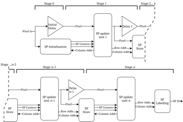
Based on this analysis, all three proposed simplifications to PPA-SLIC is used in the implemen-tation. The implementation is fully pipelined, with dedicated hardware for each iteration. With all the calculations of the iterations, in this context also called stages, implemented as separate hardware, there is no need for stage 2 to wait for stage 1 to process the whole image before start-ing the second iteration. The stages can be tightly connected, with the only constraint bestart-ing that when a pixel arrives in a stage, the stage before needs to already have decided the values for the nine spatially closest superpixel centres for that pixel. This spacing of stages, is implemented as a FIFO based delay, that is inserted on the pixel line between each iteration.
This design is able to accept a pixel every clock cycle, so in the same way as a processor that fetches a new instruction every clock cycle is said to be fully pipelined, this accelerator could be called fully pipelined. It is therefore given the name fully pipelined SLIC, or FP-SLIC.
Column Addr Pixel Initial Delay SP Initialisation Pixel In Column Addr SP update unit 1 SP Centers Delay 1 Pixel SP Store Row Addr Pixel
Stage 0 Stage 1 Stage 2...
SP Store Column Addr Pixel Column Addr SP update unit n-1 SP Centers Delay n-1 Pixel SP Store Row Addr Column Addr Pixel Column Addr SP update unit n SP Centers SP ID SP Labelling Row Addr Stage n-1 Stage n Stage ...n-2
Figure 3: Block diagram overview of FP-SLIC. Stages 2 to n − 2 are the same as stage 1 and stage n − 1. Here a minimum of three stages is shown, but there is no reason for why the pipeline can not be constructed from fewer stages. All the way down to where the initialisation stage would be followed by the labelling stage and only one SP update unit used.
As shown in Figure 3, the main stages of the accelerator consist of three parts, the before mentioned delay, the superpixel update unit, and the superpixel store.
5.2.1 Delays
The delays are implemented as FIFO ring-buffers in block RAM, they and all other parts of the pixel line driven by AXI stream valid/ready handshakes, starting on the input side as an AXI stream slave taking RGB pixels and ending on the output side as an AXI stream master pushing the superpixel ID of pixels. The length of the delays depend on the size of the image, and the grid spacing of the initial superpixel centre positions as this is used as a heuristic to approximate the nine spatially closest superpixels of pixels. This spacing is the same one introduced in the background on SLIC in section 2.1, S. Thinking of the image as a grid of S × S pixel squares, with one superpixel centre originally placed in the middle of each square, a pixel could belong to any superpixel in the 3 × 3 region of squares around it. The spacing between the first pixel that could belong to a specific superpixel, to the last pixel that could possibly belong to that superpixel, will be three rows of squares, 3 · S · w pixels, where w is the width of the image. For reasons that will be explained in section 5.2.3, stemming from how the superpixel centre values are loaded into the superpixel update units, the delay length is instead set to (3 · w + 1) · S + 1 cycles.
5.2.2 Superpixel stores
The superpixel stores hold the superpixel centre values for use in the next stage. They are con-structed from six banks of block RAM, each holding one row, i.e. w/S, of superpixels. At every instance, three of the banks are designated for the current stage to write to, and three for the next stage to read from, which three currently used for what, is decided by a counter that moves one step forward for every S rows of pixels processed in the local stage. The data that is stored for every superpixel is the sum of the pixels assigned to that superpixel, where summation of pixels
in this usage implies vector addition of pixels with the components red, green, blue, column and row. Resetting the memory space when it is to be reused for a new superpixel, is handled by the writing update unit, setting a signal called overwrite.
When assigning a new pixel to a superpixel, a read is first required, to fetch the current value from the write destination. With the block RAM in the 7-series FPGAs from Xilinx, two clock cycles are needed for this operation of reading from a cell and then writing back to it. This is not a problem for the reading side, as there will always be more than two clock cycles after a write until the update unit in the next stage will read that particular superpixel, but it might lead to a data hazard if two consecutive pixels are assigned to the same superpixel. The read of the second assignment will happen in the same clock cycle as the write of the first assignment, and the old value will therefore be added to the second pixel and written over what was just written, completely negating that first pixel. To avoid this, the incoming pixel is added to the last sum instead of the value read from its destination address in the cases where that it is the same as the address before.
On the reading side, the update unit provides a column address and is the next clock cycle given the superpixel centre value for that column from all three rows designated for reading. The values read from the block RAMs are divided by the number of pixels assigned to that superpixel, to get the mean value for the superpixel. To avoid problems with division by zero, the superpixel centre values from the superpixel store, all have an associated valid flag, which is false if the number of pixels assigned to the superpixel is zero.
5.2.3 Superpixel update units
The superpixel update unit is the component that drives the whole algorithm, assigning all incom-ing pixels to their closest superpixel and in that refinincom-ing the superpixels through the averagincom-ing in the superpixel store. The nine closest superpixels is kept track of, through a 3 sliding window, feed by the preceding superpixel store. The distance from the current pixel to these nine superpixel centres are calculated in parallel, through a minimum function tree, the sliding window index of the smallest distance is extracted. This index is converted to a row and column address for which superpixel to assign the current pixel.
The sliding window shifts the columns of superpixels it every S clock cycles. The counter that handles this is synchronised using the SOF and EOL signals that are available in the pixel AXI stream. The first shift of a frame occurs at the same time as the first pixel of a frame arrives in the superpixel update unit, so the sliding window should after that shift have the top leftmost superpixel in the middle, as this heuristically will be the spatially closest superpixel to the first S pixels. The rightmost column is directly connected to the superpixel stores outputs, and needs to contain the leftmost superpixels before the first pixel arrives, for them to be in the right place after the first shift, as shown in Figure 4.
SP 0,0 SP 1,0 SP 0,0 SP 0,1 SP 1,0 SP 1,1 SP 0,0 SP 0,1 SP 1,0 SP 1,1 SP 0,2 SP 1,2 Before first pixel. First S pixels in row 1. Second S pixels in row 1.
S S
Figure 4: Diagram of how the sliding window changes for the first few pixels of a new frame. This, and the similar need of having to load the first column again before the pixels of the next row arrives, as shown in Figure 5, is why the pixel delay between stages is S longer than it would initially seem to need to be. The extra +1 is to offset the clock cycle that the reads from the superpixel stores take.
SP 0,n
Second to last S pixels in row S. Last S pixels in row S. First S pixels in row S+1.
SP 0,n-1 SP 0,n-2 SP 1,n SP 1,n-1 SP 1,n-2 SP 1,0 SP 0,n SP 0,n-1 SP 2,0 SP 1,n SP 1,n-1 SP 0,0 SP 1,0 SP 0,n SP 2,0 SP 1,n SP 0,0 SP 1,1 SP 2,1 SP 0,1
Figure 5: Diagram of how the sliding window changes at the end of row S. This is similar for other end of rows, except for the change of superpixel row.
In all the cases shown in Figures 4 and 5, there are cells in the sliding window that contain either garbage data or irrelevant centres, rather than one of the nine spatially closest to the currently processed pixel. For all pixels closer than S pixels from the edge, and for superpixels loaded from the store with a false valid flag, the calculated distance values are replaced with the maximum distance, so that those cells are not chosen by mistake.
5.2.4 Initialisation and labelling
The first, or initialisation, stage and the last stage, i.e. stages 0 and n in Figure 3, are a bit different. The initialisation stage consists of a simplified version of the superpixel store, with no summation and no averaging. This store is updated with the pixel values from the middle of the S × S squares, as this is what the superpixels are initialised to. For the first two rows of superpixels to be set up when the first pixel reaches the first superpixel update unit, a delay is needed here as well. In this case, it only needs to be (2 · w + 1) · S + 1 long, as only the middle pixel of the square corresponding to a superpixel needs to be reached for that superpixel to be defined.
In the last stage, the row and column addresses from the update unit, that in other stages are used to write the pixel values to their assigned superpixel in upcoming superpixel stores, are instead combined to label the pixel with a superpixel ID. It is calculated as, ID = wSP· Arow+ Acol,
where wSPis the number of superpixels per row, or superpixel width, Arowis the row address and
Acolis the column address. The superpixel IDs are then written out as an AXI stream, combined
with the SOF and EOL signals from the corresponding pixels.
The output can instead be given per superpixel. Then the labelling is replaced with one last superpixel store to calculate the final values for the superpixel centres. The superpixels are then reported, as the average position and colour, as well as size in number pixels.
5.2.5 Simulation
The components are evaluated using VHDL test benches in behavioural simulations. The simulator used is the open-source VHDL simulator GHDL. This was chosen due to its better support of the VHDL-2008 standard compared to the simulator shipped with Xilinx Vivado.
First, components are simulated separately to verify that they behave as specified. Most of the test benches use pseudo random generated values to test a wide range of possible inputs. To automate this verification process, assert statements are used to check the outputs when pos-sible without too complex calculations on the test bench side, for example in testing the basic functionality of the superpixel store.
Test benches are then developed for testing the algorithm as a whole. Initially, the algorithm is tested with pixels of a constant value and after that random values. The output waveforms are analysed to verify that the dataflow is correct and that counters and other signals that should be synchronised between different stages and components are. Finally, a test bench is used that loads an image from a file and writes the output to a .csv file; this is first tested with small and simple images, as running these simulations takes multiple hours, and the simulation time scales with the image size. When these small images are segmented in a way that seems correct, simulations are instead run with the full sized images from the BSDS500, so the segmentation can be evaluated
quantitatively. The execution time of these simulations limits the possibility to do enough runs to calculate any quality metrics that would be statistically significant for the implementation, as done for the high-level implementation. Undersegmentation error and boundary recall are still calculated for the few simulations completed.
5.3
FPGA implementation and testing
The next step is to implement and run the VHDL design on an FPGA. The device targeted is the Xilinx Zynq-7020, as this is the FPGA SoC on the GIMMIE2 computer vision system used by Carl. It should be noted that the board actually used in the end was the Snickerdoodle Black4
from Krtkl, but it is designed around the same SoC as the GIMMIE2.
To stream pixels in and out of the superpixel accelerator, the VDMA5 IP core from Xilinx is
used. Due to limitations of the implementation, the tready signal of the outgoing AXI stream is required to be kept high, so to accommodate that and to pick up slack in the stream, a FIFO buffer is added after the FP-SLIC module and before the write side of the VDMA module.
On the software side PYNQ is used, as it provides a simple and fast way to set up the VDMA data transfer. The availability of a precompiled PYNQ image for it is why the Snickerdoodle Black board is used. Images from the BSDS500 are again used to test the implementation.
6
Results
In this section the results of the thesis are presented. Starting with the high-level implementation, showcasing the segmentation quality through quantitative measurements. Then comes visualisa-tions of the outputs from simulating the low-level implementation, and lastly visualisavisualisa-tions of the FPGA output and data on the resource usage of the FPGA implementation.
6.1
High-level implementation
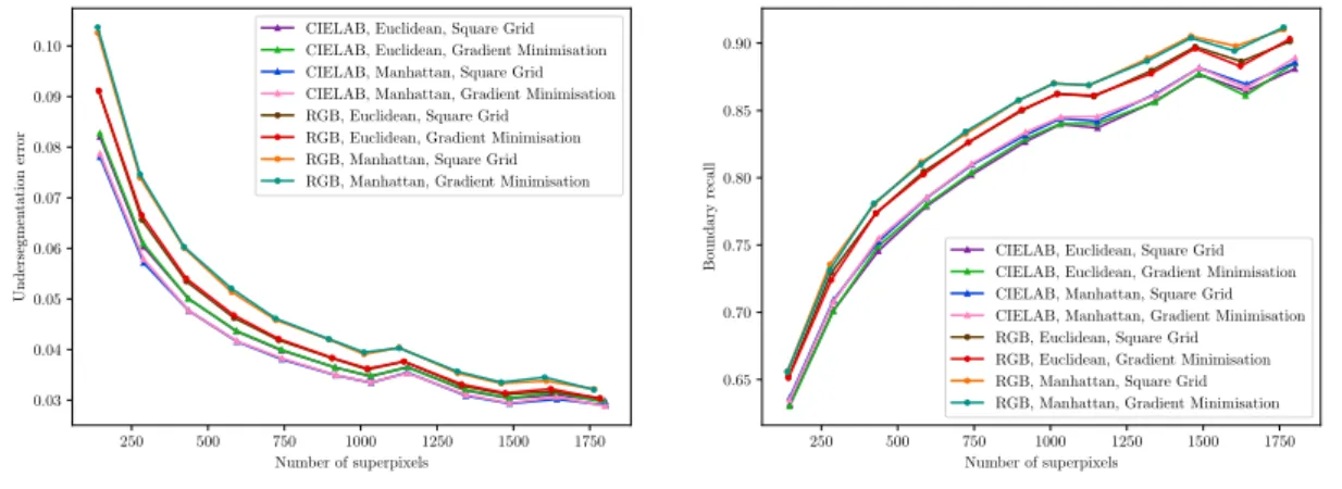
The results from evaluating the high-level implementation against the BSDS500 dataset are shown in Figures 6 to 8. In these plots, undersegmentation error and boundary recall are used as a measure of superpixel segmentation quality. For a definition of these metrics, see Section 2.2. Each data point represents the mean value from all 500 images in the data set.
In Figure 6 undersegmentation error and boundary recall have been plotted against the num-ber of superpixels that the used images have been segmented into to show how the quality of segmentation correlates to the granularity of that segmentation.
250 500 750 1000 1250 1500 1750 Number of superpixels 0.03 0.04 0.05 0.06 0.07 0.08 0.09 0.10 Undersegmen tation error
CIELAB, Euclidean, Square Grid CIELAB, Euclidean, Gradient Minimisation CIELAB, Manhattan, Square Grid CIELAB, Manhattan, Gradient Minimisation RGB, Euclidean, Square Grid RGB, Euclidean, Gradient Minimisation RGB, Manhattan, Square Grid RGB, Manhattan, Gradient Minimisation
250 500 750 1000 1250 1500 1750 Number of superpixels 0.65 0.70 0.75 0.80 0.85 0.90 Boundary recall
CIELAB, Euclidean, Square Grid CIELAB, Euclidean, Gradient Minimisation CIELAB, Manhattan, Square Grid CIELAB, Manhattan, Gradient Minimisation RGB, Euclidean, Square Grid RGB, Euclidean, Gradient Minimisation RGB, Manhattan, Square Grid RGB, Manhattan, Gradient Minimisation
Figure 6: Comparisons between different versions of PPA-SLIC.
4https://krtkl.com/snickerdoodle
5Video Direct Memory Access https://www.xilinx.com/support/documentation/ip_documentation/axi_vdma/ v6_2/pg020_axi_vdma.pdf
In Figure 7 PPA-SLIC is compared to SNIC and generic CPA SLIC, which both can be con-sidered state-of-the-art. Figure 8, where superpixel quality is plotted against the used number of iterations, also shows PPA-SLIC compared against state-of-the-art algorithms, but it was mainly included to help in deciding what iteration depth to use in low-level implementation.
250 500 750 1000 1250 1500 1750 Number of superpixels 0.03 0.04 0.05 0.06 0.07 0.08 0.09 0.10 Undersegmen tation error SNIC SLIC PPA-SLIC PPA-SLIC simplified 250 500 750 1000 1250 1500 1750 Number of superpixels 0.5 0.6 0.7 0.8 0.9 Boundary recall SNIC SLIC PPA-SLIC PPA-SLIC simplified
Figure 7: Comparisons between PPA-SLIC and the state-of-the-art superpixel segmentation algo-rithms SLIC and SNIC.
2 4 6 8 10 12 14 16 Iterations 0.036 0.038 0.040 0.042 Undersegmen tation error SLIC PPA-SLIC PPA-SLIC simplified 2 4 6 8 10 12 14 16 Iterations 0.74 0.76 0.78 0.80 0.82 0.84 0.86 Boundary recall SLIC PPA-SLIC PPA-SLIC simplified
Figure 8: Evaluation of segmentation quality depending on the number of iterations run.
6.2
Simulation of low-level implementation
In this section results are presented from simulations were the FP-SLIC implementation was tested with images from BSDS500. All simulation runs were done with the FP-SLIC implementation configured to 3 iteration stages, approximately 1600 superpixels, and the compactness factor m sat to 80.
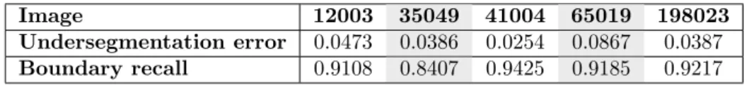
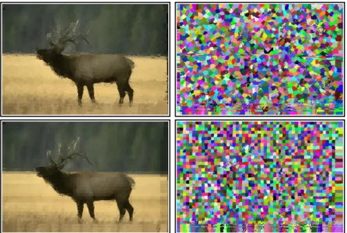
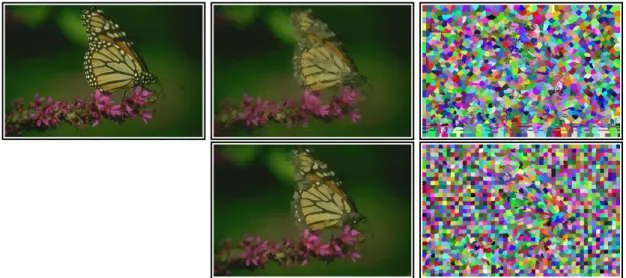
With the 481 × 321 pixel images of the BSDS500 data set, the simulations took up to 12 hours on a computer with an Intel i7-6500U CPU running at 2.50GHz and 16GB of memory. Hence only five images from BSDS500 were tested in simulation. Table 1 shows the superpixel segmentation quality metrics of undersegmentation error and boundary recall for the outputs from these five runs. The superpixel output for image 41004, both from the FP-SLIC simulation and from the high-level implementation of the simplified PPA-SLIC, are visualised in Figure 9. The same for the other four evaluated images can be found in Appendix A.
Image 12003 35049 41004 65019 198023
Undersegmentation error 0.0473 0.0386 0.0254 0.0867 0.0387
Boundary recall 0.9108 0.8407 0.9425 0.9185 0.9217
Table 1: Results from evaluating the behavioural simualtion of FP-SLIC against BSDS500.
Figure 9: Comparison between outputs from the high-level implementation of simplified PPA-SLIC and a simulated implementation of FP-SLIC when segmenting BSDS500 image 41004. The top image is the original, the middle images are based on the FP-SLIC output and the bottom ones on the PPA-SLIC output. The left images are the superpixel outputs with superpixels coloured as the average colour of pixels in that superpixel, and to the right every superpixel is given a random colour.
6.3
FPGA implementation
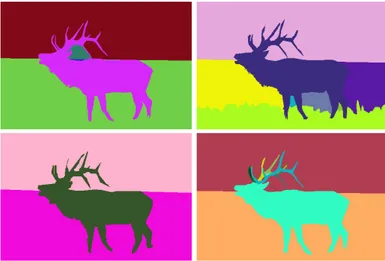
The maximum frequency where the implementation met timing constraints of the FPGA is about 10MHz, resource utilisation of the implementation can be seen in Tables 2 and 3, for one and three stage versions respectively. Superpixel outputs from these two versions of the implementation can be seen in Figure 10.
Resource Utilisation Available Utilisation %
LUT 5074 53200 9.54
LUTRAM 227 17400 1.30
FF 5144 106400 4.83
BRAM 23 140 16.43
BUFG 1 32 3.13
Table 2: FPGA resource utilisation for a single stage implementation
Resource Utilisation Available Utilisation %
LUT 21496 53200 40.41
LUTRAM 227 17400 1.30
FF 10011 106400 9.41
BRAM 85 140 60.71
BUFG 1 32 3.13
Table 3: FPGA resource utilisation for a three stage implementation
Figure 10: Visualisations of the output from the FPGA implementation for BSDS500 image 41004. The top images are from the algorithm set to three iteration stages, and the bottom images are from it set to one iteration stage. To the left, superpixels are set to the mean colour of pixels in that superpixel, and to the right, superpixels are given a random colour.
7
Discussion
In this section the results of the thesis are discussed and analysed. Improvements and future work are also introduced, and the research questions answered.
7.1
High-level implementation results
The evaluation of the high-level implementation had three main outcomes. Firstly, Figure 7 shows that PPA-SLIC can compete against state-of-the-art algorithms like SLIC (CPA-SLIC) and SNIC in terms of superpixel quality. This is consistent with the results presented by Hong et al. [19], as they show that the PPA based algorithm S-SLIC generates superpixels of similar or higher quality than SLIC.
Secondly, the three proposed simplifications to SLIC, i.e. changing the Euclidean distance met-ric to Manhattan distance, leaving out the gradient minimisation from the initialisation superpixel centres, and changing the colour space from CIELAB to RGB, had no significant ill effect on the quality of superpixel segmentation. Looking at Figure 6, it becomes clear that the removal of the gradient minimisation step has the least impact of the three simplifications. In both the under-segmentation error and boundary recall plots, the eight configurations of PPA-SLIC can be seen as four pairs of graphs, with very little difference between the two members pairs of each pair. What links the configurations, in all four of these pairs, are that they adopt the same colour space and distance metric within a pair, but one of them includes the gradient minimisation step, and the other one does not. The impact of the other two simplifications are greater, but still small. Between the two, the colour space has the bigger impact. The use of the RGB colour space instead of CIELAB has a positive effect on boundary recall, showing a slight increase, but a negative effect on the undersegmentation error, showing a similar increase. Comparing distance metrics, shows a similar picture, the use of Manhattan distance results in a higher boundary recall, especially when combined with the RGB colour space. When looking at the undersegmentation error, the impact is less clear. Manhattan distance increases the undersegmentation error when combined with the RGB colour space, but shows a decrease when used with CIELAB. To summarise, the configuration of PPA-SLIC that would be most beneficial for FPGA implementation, i.e. all three simplifications combined, is no better or worse for superpixel quality than the generic version of PPA-SLIC. It comes down to if high boundary recall or low undersegmentation error should be valued higher. With a higher boundary recall, the simplified version of PPA-SLIC will output superpixels that adhere better to natural boundaries and edges compared to the generic version of PPA-SLIC, but with an equally higher undersegmentation error value, the risk of it placing multiple close features, that should have been distinct clusters, in the same superpixel is also higher.
Thirdly, Figure 8 shows that for PPA-SLIC, the major improvements in segmentation quality happen in the first two or three iterations, and after six iterations there are nearly no increases. For generic CPA-SLIC, the quality increase over iterations are instead more gradual but lasts for longer. This is again a result in line with the findings of Hong et al. [19] Their comparison of memory usage showed, that a nine centre region of interest PPA algorithm has a higher pixel-to-centre ratio than a 2S × 2S pixel region of interest CPA algorithm. For a CPA algorithm to have an equivalent pixel-to-centre ratio, it would have a 3S × 3S region of interest. Using more pixels to redefine the centres in every iteration, is analogous to increasing the step size in minimising the pixel to centre distance. This explains why the CPA SLIC can continue to improve its superpixel quality for longer, as it adopts a smaller step size. As with a fixed step size in gradient descent, a smaller step size will lead to a lower rate of convergence, but if the step size is too big, then the optimisation might miss the optimum.
7.2
Low-level implementation results
The undersegmentation error and boundary recall values from simulation of FP-SLIC shown in Table 1 are close to the ones for the high-level implementation of PPA-SLIC in Figure 7, but as can be seen when comparing the segmentations from these in Figure 9 or Appendix A, the outputs are quite different. The high-level implementation of simplified PPA-SLIC generates more rectangular superpixels, and as can be seen along the left and bottom edges of the outputs from the FP-SLIC simulation, it also encodes some vertical and horizontal artefacts on the output. The artefacts are the result of one or more bug in the code, yet to be determined and resolved. The question of why the superpixels are looking more like a Voronoi diagram, than the almost grid of the output of the high-level implementation, is trickier. With some bugs still present, it is hard to say if this is a property of the intended differences between simplified PPA-SLIC and FP-SLIC or if this as well is a product of the bugs in FP-SLIC. One thing that is known is that it increases with the
number of iteration stages, in Figure 10, the superpixels from the single stage pipeline are more square than those from the three stage pipeline.
The non squareness of these superpixels does not affect the boundary recall and undersegmena-tion error value, and at least for the five images evaluated in simulaundersegmena-tion, the left and bottom edges do not contain enough detail for the artefacts to disrupt more than a few ground truth segments. Another reason for these quality metrics to be so good, even when the segmentation looks worse to human eyes in comparison to the segmentation by the high-level implementation, is the high amount of superpixels used in comparison to the resolution of the ground truth. Examples of the ground truths from BSDS500 is shown in Figure 11, they all contain much bigger segments than those of normally generated by superpixel aglorithms, as the BSDS is a generic data set for segmentation and not made specifically for superpixel segmentation. Undersegmentation error is
Figure 11: Visualisations of BSDS500 groundtruths for image 41004.
calculated per superpixel and ground truth segment pair, and boundary recall is calculated for the border pixels of the ground truth, so with many superpixels, areas of higher undersegmentation error averages away, and with such a high ratio between ground truth segment size and superpixel size, very few of the superpixels actually participate in the calculation of boundary recall. For this reason, undersegmentation error and boundary recall are often compared over different number of superpixels, as done for the high-level implementation, but due to time constraints and long run times, this has not been possible with the simulation of FP-SLIC.
The segmentation output from FP-SLIC running on an FPGA, seen in Figure 10, is mostly the same as the output from the simulation, seen in Figure 9. The only difference apparent to visual inspection is that in addition to the artefacts in the simulation, the FPGA outputs, also have some horizontal lines where the pixels seems to have been offset to the right. When comparing the output from the three and one iteration runs, the offset looks identical, both in vertical spacing and size. This pipeline depth invariance, and that this problem does not show up in the simulation points to that the problem lies in how FP-SLIC interacts with the VDMA block. In the simulation test bench, the AXI stream interfaces behave nicely, with the master constantly valid, and the slave constantly ready. The VDMA block does not behave in this way, so the creation of a meaner test bench, to help in the creation of an AXI stream chain that is more robust to starting and stopping, should be one of the first steps in the continued development of FP-SLIC. The AXI stream running through the whole algorithm, is the most vulnerable part of the design, as it is what connects the algorithm to the outside, and what propagates the information through the iteration stages, therefore it is crucial that it works as specified. The well known and well defined nature of the AXI stream specification makes formal verification a viable solution to checking the correctness of the AXI stream implementation. Formal verification was considered outside the scope of this thesis but is absolutely something to look at in the future work on this algorithm.
Even if the FPGA superpixel accelerator developed by Miyama, is based on a different algo-rithm, it can still be interesting to compare the resource usage and throughput of FP-SLIC against it. Miyamas SEEDS implementation [20] uses more of all FPGA resource types than FP-SLIC, at
least for one and three implementation stages, see Tables 2 and 3 for FP-SLICs resource usage; and his implementation also use five external RAM chips. If this comparison is taken as an indication, then FP-SLIC can be considered an inexpensive implementation of superpixel segmentation, in terms of resource usage. Miyamas SEEDS implementation can achieve 42.2 FPS on 640 × 480 pixel images, the theoretical throughput for FP-SLIC running at 10MHz is 32.6 FPS for the same image size. The lower throughput of FP-SLIC is entirely a product of the lower clock frequency, Miya-mas SEEDS runs at 30MHz and processes on average 0.43 pixels per second, whereas FP-SLIC can process new pixel every clock cycle. So if the max frequency of FP-SLIC could be increased, then much higher image throughputs could be reached. The distance calculations and comparisons of the superpixel update unit in FP-SLIC are currently all done in the same clock cycle, splitting this into two or three pipelined stages should be the first step in trying to increase the max frequency.
7.3
Research questions
Combining the results and analysis of this thesis, two of the set research questions can be answered satisfyingly. Answers to these questions, and a short analysis of what has stopped this work from answering the remaining two, are presented below.
Q1. What algorithm, or algorithms, do other research point to as state-of-the-art in superpixel segmentation?
SLIC stands out as the superpixel segmentation algorithm that is most prominently used in re-search. SLIC is also shown to have good and balanced results on a lot of different parameters, by the comparisons of superpixel segmentation algorithms done by Neubert and Protzel [10], and Stutz et al. [22].
Q2. Can the superpixel segmentation algorithms from Q1 be implemented on an
FPGA?
Yes. Even if the FPGA implementation of SLIC created is this thesis requires more work to be considered done, and to be usable in a real application; it still functional enough to be able to say that it is possible to implement SLIC on an FPGA.
Q3. What are the advantages of implementing superpixel segmentation on an FPGA? Q4. What are the limitations of superpixel segmentation implemented on an FPGA? Q3 and Q4 could not be answered, as final evaluations of the FPGA implementation have not been possible with the current state of the implementation. Though the results available indicate that the FPGA implementation should be both fast and resource efficient if the remaining bugs in it can be resolved without too drastic changes.
8
Conclusion
In this thesis, it was attempted to create a hardware accelerator for superpixel segmentation, on an FPGA. To accomplish this, an iterative engineering methodology was established. The first step was to research different algorithms for superpixel segmentation; this concluded in the design of an algorithm based on the iterative algorithm SLIC. Much inspiration for this algorithm was taken from the paper A real-time energy-efficient superpixel hardware accelerator for mobile computer vision applications [19]; the main takeaway was the concept of a pixel perspective architecture, PPA. Three simplifications to this algorithm, i.e. PPA-SLIC, were identified to reduce the com-plexity of an FPGA implementation of the algorithm. PPA-SLIC was then implemented in the high-level programming language C++. The high-level implementation was evaluated against the Berkeley Segmentation Data Set, calculating the quality metrics boundary recall and underseg-mentation error. The evaluation showed, that PPA-SLIC, with the three simplifications, generated superpixels of similar quality to those from state-of-the-art superpixel segmentation algorithms and that a low number of iterations, in the range of about one to four, is sufficient for the output
of PPA-SLIC to converge on a high quality segmentation. Based on these results, a fully pipelined FPGA implementation of PPA-SLIC was developed in VHDL. The implementation runs on real hardware, and can successfully segment an image into superpixels, but there are some issues with robustness, and the segmented output contains some visual artefacts. To solve these issues, and to increase the speed of the implementation, more work is required, and this will continue outside the confines of the thesis work.
Acknowledgement
I would like to thank my supervisor Carl Ahlberg for all the help and support he has provided during the thesis process, and for proposing such an interesting topic.
References
[1] Ren and Malik, “Learning a classification model for segmentation,” in Proceedings Ninth IEEE International Conference on Computer Vision, Oct 2003, pp. 10–17 vol.1.
[2] M. Miyama, “Fast stereo matching with super-pixels using one-way check and score filter,” in 2017 7th IEEE International Conference on Control System, Computing and Engineering (ICCSCE), Nov 2017, pp. 278–283.
[3] F. Gu, H. Zhang, and C. Wang, “A Classification Method for Polsar Images using SLIC Superpixel Segmentation and Deep Convolution Neural Network,” in IGARSS 2018 - 2018 IEEE International Geoscience and Remote Sensing Symposium, July 2018, pp. 6671–6674. [4] R. Achanta, A. Shaji, K. Smith, A. Lucchi, P. Fua, and S. S¨usstrunk, “Slic superpixels,” 2010.
[5] M. R. Luo, CIELAB. Berlin, Heidelberg: Springer Berlin Heidelberg, 2014, pp. 1–7.
[Online]. Available: https://doi.org/10.1007/978-3-642-27851-8 11-1 (Accessed 2020-01-30). [6] R. Achanta and S. Susstrunk, “Superpixels and polygons using simple non-iterative
cluster-ing,” 07 2017, pp. 4895–4904.
[7] M. Van den Bergh, X. Boix, G. Roig, B. Capitani, and L. Van Gool, “SEEDS: Superpixels Extracted via Energy-Driven Sampling,” in International Journal of Computer Vision, vol. 111, 10 2012.
[8] F. Meyer, “Color image segmentation,” in 1992 International Conference on Image Processing and its Applications, April 1992, pp. 303–306.
[9] P. Neubert and P. Protzel, “Compact Watershed and Preemptive SLIC: On Improving Trade-offs of Superpixel Segmentation Algorithms,” in Proceedings - International Conference on Pattern Recognition, 08 2014, pp. 996–1001.
[10] P. Neubert and P. Protzel, “Superpixel benchmark and comparison,” in Forum Bildverar-beitung, 2012.
[11] D. Martin, C. Fowlkes, D. Tal, and J. Malik, “A database of human segmented natural images and its application to evaluating segmentation algorithms and measuring ecological statistics,” in Proc. 8th Int’l Conf. Computer Vision, vol. 2, July 2001, pp. 416–423.
[12] P. Arbelaez, M. Maire, C. Fowlkes, and J. Malik, “Contour detection and hierarchical image segmentation,” IEEE Trans. Pattern Anal. Mach. Intell., vol. 33, no. 5, pp. 898–916, May 2011.
[13] P. R. Schaumont, A Practical Introduction to Hardware/Software Codesign, 1st ed. Springer
Publishing Company, Incorporated, 2010.
[14] iCE40 UltraPlus Family Data Sheet, FPGA-DS-02008 aug 2017 ed., Lattice Semiconduc-tor Corporation, [Online; accessed 08. Feb 2020] https://www.mouser.se/datasheet/2/225/ iCE40%20UltraPlus%20Family%20Data%20Sheet-1149905.pdf.
[15] C. Ahlberg, F. Ekstrand, M. Ekstrom, G. Spampinato, and L. Asplund, “Gimme2 - an embed-ded system for stereo vision and processing of megapixel images with fpga-acceleration,” in 2015 International Conference on ReConFigurable Computing and FPGAs (ReConFig), Dec 2015, pp. 1–8.
[16] AMBA 4 AXI4-Stream Protocol, 1st ed., ARM, [Online; accesed 11. May 2020] https://static. docs.arm.com/ihi0051/a/IHI0051A amba4 axi4 stream v1 0 protocol spec.pdf, 2010.
[17] AXI4-Stream Video IP and System Design Guide, Ug934 ed., Xilinx, [Online; accesed 11. May 2020] https://www.xilinx.com/support/documentation/ip documentation/axi videoip/ v1 0/ug934 axi videoIP.pdf, oct 2019.
[18] (2020, Feb) PYNQ Introduction — Python productivity for Zynq (Pynq). [Online; accessed 14. May 2020]. [Online]. Available: https://pynq.readthedocs.io/en/v2.5.1
[19] I. Hong, I. Frosio, J. Clemons, B. Khailany, R. Venkatesan, and S. W. Keckler, “A real-time energy-efficient superpixel hardware accelerator for mobile computer vision applications,” in 2016 53nd ACM/EDAC/IEEE Design Automation Conference (DAC), June 2016, pp. 1–6. [20] M. Miyama, “Fpga accelerator for super-pixel segmentation featuring clear detail and short
boundary,” in IIEE J Transactions on Image Electronics and Visual Computing, vol. 5, 2017, pp. 83–91.
[21] M. Miyama, “HD 180 FPS FPGA Processor to Generate Depth Image with Clear Object Boundary,” in 2019 2nd International Symposium on Devices, Circuits and Systems (ISDCS), March 2019, pp. 1–4.
[22] D. Stutz, A. Hermans, and B. Leibe, “Superpixels: An evaluation of the state-of-the-art,” CoRR, vol. abs/1612.01601, 2016. [Online]. Available: http://arxiv.org/abs/1612.01601
A
Image Segmentations
Figure 12: Comparison between outputs from the high-level implementation of simplified PPA-SLIC and a simulated implementation of FP-PPA-SLIC when segmenting BSDS500 image 12003. The top left image is the original, the images to the right of that are based on the FP-SLIC output and the bottom ones on the PPA-SLIC output. Of the segmentations, the left images are the superpixel outputs with superpixels coloured as the average colour of pixels in that superpixel, and to the right every superpixel is given a random colour.
Figure 13: Comparison between outputs from the high-level implementation of simplified PPA-SLIC and a simulated implementation of FP-PPA-SLIC when segmenting BSDS500 image 35049. The top left image is the original, the images to the right of that are based on the FP-SLIC output and the bottom ones on the PPA-SLIC output. Of the segmentations, the left images are the superpixel outputs with superpixels coloured as the average colour of pixels in that superpixel, and to the right every superpixel is given a random colour.
Figure 14: Comparison between outputs from the high-level implementation of simplified PPA-SLIC and a simulated implementation of FP-PPA-SLIC when segmenting BSDS500 image 65019. The top left image is the original, the images to the right of that are based on the FP-SLIC output and the bottom ones on the PPA-SLIC output. Of the segmentations, the left images are the superpixel outputs with superpixels coloured as the average colour of pixels in that superpixel, and to the right every superpixel is given a random colour.
Figure 15: Comparison between outputs from the high-level implementation of simplified PPA-SLIC and a simulated implementation of FP-PPA-SLIC when segmenting BSDS500 image 198023. The top left image is the original, the images to the right of that are based on the FP-SLIC output and the bottom ones on the PPA-SLIC output. Of the segmentations, the left images are the superpixel outputs with superpixels coloured as the average colour of pixels in that superpixel, and to the right every superpixel is given a random colour.