Longitudinal road profiling by measurement of coordinates and slopes : A comparison between two different measuring systems

STATENS VAG OCH TRAFIKINSTITUT

National Swedish Road and Traffic Research Institute

LONGITUDINAL ROAD PROFILING BY MEASUREMENT

OF COORDINATES AND SLOPES, A COMPARISON

BETWEEN TWO DIFFERENT MEASURING SYSTEMS

by

Olle Andersson and 0116 Nordstrém

REPORT No. 25 A

STATENS VAG- OCH TRAFIKINSTITUT

National Swedish Road and Traffic Research Institute

LONGITUDINAL ROAD PROFILING BY MEASUREMENT

OF COORDINATES AND SLOPES, A COMPARISON

BETWEEN TWO DIFFERENT MEASURING SYSTEMS

by

Olle Andersson and 0116 Nordstrém

REPORT No. 25 A

Preface

The following report describes part of the work on the development

of two different systems for measurement of longitudinal road profiles, which has been carried out at the Swedish Road and Traffic Research Institute in recent years. One system (DFl) was

developed by the mechanical department of the institute in the

previous organization, and the other system (CHLOE) was dealt with by the road base department. The two activities were later joined and the present report is limited to a comparative study Sponsored by the Road Administration.

In addition to the authors, contributions to the work have been made by Hans Runqvist, who built the DFl system and developed

the measuring system around it, Brajnandan Sinha, who made the computations and evaluations of the DFl data. The measurements and datalogging in conjunction with the CHLOE measurements and the arrangements of the test sections were made by Torbjorn Linden. The report was issued in Swedish in March 1973. After that the report has been slightly revised and thereby adjusted for an inter-national audience and written in English. In the meantime the

measuring system of the CHLOE meter has been exchanged. The

movement of the vertical measuring arm is now measured by means of an LVDT, whose output via a digital voltmeter is transmitted

to a paper tape punch. On the tape is recorded the slope of

the measuring wheels in milliradians once every 15th

centi-meter of travel.

Stockholm Au ust 1973

/

Olle Andersson

Summary

An investigation of the correlation between the motorist's

judge-ment of the unevenness of the road surface and the root mean square slope as measured by the CHLOE meter was performed in the autumn of

1970 by rating and measurements of 23 test sections in the

surroundings of Stockholm. These data and measurements made by

means of a measuring system made at the institute and based upon

the GM road profiler were used for a comparison of these two

measuring systems. The correlation between the rating on one hand and the root mean square slope, the comfort index, the road

holding index and the impact factor was studied. Some further

parameters derived from the CHLOE data were also studied as well

as the Fourier spectra of the profiles according to both measuring systems. The correlation coefficients were about 0.7. Advantages and disadvantages of the two measuring systems are discussed.

Longitudinal road profiling by measurement of c00rdinates and slopes, a comparison between two different measuring systems.

Introduction_ ~

The longitudinal profile of a road is the intersection between the road surface and a vertical plane through.the longitudinal direction of the road. It may be useful to distinguish between three different orders of magnitude of the profile.

1. The country prOfile. Profile details whose extension is larger than 1 10 meters.

2. The evenness profile. Profile details in the interval 0.1 -10 meters.

3. The surface texture. Profile details less then 0.1 meter extension.

The dividing points between these three catagories is quite arbi-trary, and the terminology used here was invented for the.

sake of discussion. The following report is limited to alterna-tive 2, the evenness profile. The term "evenness profile" was used because it is felt that profile wave lengths in this order' of magnitude are the main causes of the feeling of unevenness and bumpiness felt by the motorist and influencing the transported goods. The most simple device for determination of such profiles'

is a straightedge, whose vertical distance from the road surface is measured by some_sort of length gauge. This method is however tedious and laborious, and the length of the straight-edge is often unsatisfactory, or the device becomes clumsy.

Numerous automatic devices for longitudinal profiling have been iconstructed. In a thesis by Lehtinen (l) som fifty different

devices are referred to. One of the simplest and moat used

devices is the mechanized straight-edge. This device records the vertical road surface coordinates automtically. The base line

(i.e. the-straight-edge) is however not stationary, neither its direction nor its location, and the result of the measurement is therefore debatable. /

The work described in this report deals with a Comparison between the CHLOE meter, which is a slope meter, and an electronic

coordinate meter, originally designed by GM, the version built _ at Our institute being denominated DFl.

Measuring apparatus

~ - -. .- - _n . ~u_

The DFl system was described in Internal Report 65 from the Road Research Institute and is based upon a measuring principle

deve-loped by the General Motor Corporation (2), fig 1 and 2. A pivoting

arm attached to a vehicle, preferably a passenger car, carries

a small wheel which follows the road surface. The vertical motion of this wheel relative to the car body is recorded by means of

a straight potentiometer. On the floor of the body there is an

accelerometer, which by double integrationconverts the vertical motion of the body to an electrical signal. The difference

between the two signals thus obtained is proportional to the vertical coordinate of the road surface. In the ideal case the output from this operation would give the profile of the road

surface relative to a fixed coordinate system. This is however'not

technically feasible and not even desired, since the evenness profile is limited to profile details in a limited interval of extension, and the limits of this interval can be realized in

the apparatus by setting the frequency limits of a band pass

filter. Otherwise expressed, the length of the reference line is adjustable. During measurement the signal is recorded on a magnetic tape, which is then porcessed in a computer. Measure ments can be made at normal driving speeds, and hence the measuring capacity is considerable. On the other hand certain difficulties are met in measurements of short test sections,

since the filters are not adapted to creeping speeds.

The CHLOE meter was developed in conjunction with the AASHO tests at the end of the fifties (3), fig 3 and 4. The meter is towed behind a passanger car and has one axle. Two measuring wheels are arranged longitudinally at 22.5 cm (9 ) distance in the middle between the travelling wheels The slope of the holder of the two measuring wheels equals the slope of the road surface and the slope of this holder relative to the frame of the vehicle is measured by electrical devices. The towing bar is 7 meters long, and a reading is taken once every 15th centi meter (6") along the road.

The CHLOE meter is recommended to run at maximum 5 mph, although

at our institute a limit of 5 km/h has been set, since it has appeared to bounce on certain types of road surfaces. There are

no difficulties in making measurements on short sections, although the normal length used is 150 meters, corresponding to l 000 readings.

The automatic datalogger provided by the manufacturer has been

replaced by a punch tape and some other circuitry, which makes

it possible to make full analysis of the profile in a large

computer. On particularly rough road surfaces, e.g. surface

dressings, the mechanical measuring system vibrates quite severly,

which makes the apparatus inapplicable to such roads and presum~ ably also to roads with rolled in chippings, a surfacing type whiCh has become quite popular lately due to its resistance to wear by studded tires.

Evaluationn u-u u n

The tape recorded output from the DFl is processed in an analog computer or in a digital computer after digitalization. Both methbds have been tried. Three characteristics have been computed

comfort index road holding index impact factor

The comfort index (K) is a measure of the driver's impression of

vertical motion. The index was suggested by VDI (Verein Deutscher Ingenieure) and is recommended in VDI 2057, which synthesizes I what predominantly German researchers have found regarding human response to vertical motion. The index can attain values between zero and 100 where 0 implies the absence of vertical motions and 100 corresponds to unbearable vibrations. The index can be mathe matically described by the expression

where

a = 18, a constant

2 = vertical acceleration f = frequency

0 = reference frequency = 10 Hz

The relation between comfort value, acceleration and frequency is illustrated in fig 5. It is seen that at the same acceleration the sensitivity of the driver decreases at increasing frequency

according to a hyperbola function. K values between 1 and 3 have been_classed by Mitschke (5) as normal comfort, bearable for

several hours. The interval 3 - 10 is characterized as incomfort able, bearable for not more than one hour, whereas values from 10 to 30 are characterized as strong vibrations bearable for

maximum 10 minutes. Values higher than 30 describe an extremely

uncomfortable situation which can be withstood fore one minute at the maximum. This classification can of course only give an indication of the meaning of the scale.

When an automobile runs on a road the amplitude and frequency vary irregularly. In computation of the comfort index the acceleration signal therefore has to be transmitted through a low pass filter, tuned in such a way that the proper amplitude reduction at increasing frequency is attained. Then the Signal

is squared and is sent through a low pass filter tuned i such

a way that the mean over the wanted period results. Finally the square root of the mean is computed and the result is multiplied

by the constant a. The comfort value is thus computed continously

and represents the interval between the present time and the time in the past at the distance T. The period T was in the present investigation made to correspond to a road length of 50 meters

at the speeds 20 and 25 m/s, i.e. 2.5 and 2 seconds.

The road holding index (R) is intended to give a measure of the -efficiency of braking without locking of the wheels having the

greatest load variations. This is usually the rear wheels. From stability point of View road holding of the rear wheels is the most important, which is a reason for choosing them as characteri-zing the road holding.

M

The road holding index is conceived as follows. When braking a vehiéle on a flat horizontal road a friction force equal to u - P_stat can be utilized,-where u = brake force coefficient and

PStat = static wheel load. On an uneven road the force exerted

by the wheel varies with time and is denoted by P. It is assumed that P varies symmetrically around PS_tat' When P is greater than

P_stat the brake force transmitted is u ° P_stat and at smaller

Values of P the transmitted brake force is u - P. The time average of the transmitted brake force divided by PS is defined as the road holding index (R). In this line of :::soning the moment of inertia of the wheel has been neglected. The moment of inertia

actually causes a better road holding than is accounted for by the simplified model.'Lacking a more developed parameter, the road holding index is so far used as a measure of road holding. The meaning of the road holding index (R) is illustrated in figure 6.

The road holding index is calculated continuously. The signal thereby .passes a low pass filter tuned in such a way that the index

calculated at one instant is representative of the preceding 20 meter interval. This length of interval was chosen to comply with

a time interval of 0.8 1 sec in the speed interval 20 r 25 m/sec,

-the shortest time interval allowed by the measuring system. The impact factor is a measure of the dynamic wheel load and is the ratio of the peak load and the static load. Since in real traffic on a road there is no constant peak load, in the present measurements the load exceeded 10% of the time was used as a measure of the peak load. The procedure is illustrated in the

sketch below. __ v ' .-. .-. ~- mm...H... a-.-.. ,.~...-...t_... w

I

~'. '

' '

'

i

..

>--

. .JL-iz

f?

w

'

[\j

A '/ \ /\ /\- /\

, \\.// x]? I ; . . \k//

V.

slat. \ .ax\

.

L P

l

4 m m . . . -1 H -~ .lif

I

-H H 4!

2

_T.i.

3 *4-

_:rgO? VTI. Report No 25 A

In the present study the three parameters thus introduced were computed from wheel loads and accelerations resulting from

pro-cessing DFl tapes in an analog computer programmed with a

mathe-matical model of a reference vehicle (passenger car). The mathe~

matical model has been described by Sinha (7).

The slope readings from the CHLOE meter are used for computation

of slope variance and standard deviation with respect to the mean. During the AASHO experiments an empirical relation between the

"present serviceability rating" and some pertinent road surface properties was worked out, the dominant road property being the

slope variance. The quantity calculated by this empirical formula

was denoted the "present serViceability index" PSI, ranging from

the value 5 for an excellent road and down towards O. The range

1 1/2 2 1/2 indicates the need of repair. In Sweden a series

of trial runS'was performed. Thereby 23 road sections, eachn 300 meters in length, were measured by the CHLOE meter and after~

wards rated by 75 persons driving or riding in private passenger cars. From these ratings an empirical relation was found between

the ratings and the RMS slope as measured by the CHLOE meter.

The index calculated by this formula is called TRAC, derived

from the words trafficability and E LOE (6). The TRAC scale

also runs from 1 to 5.

Since each reading from the CHLOE meter is a slope of a curve segment, integration can yield the curve itself and differentia tion once or twice will yield the second derivative, i.e. the curvature, or the third derivative. The individual values can also be used for Fourier analysis of the longitudinal profile or other more advanced curve analysis, provided a computer with a large memory capacity is available (8).

Results from measurements with;DEl__

Of the 23 road sections referred to in the above mentioned experi

ment one month after the trial 22 of the sections were tested

by DFl. In the meantime one of the sections had been resurfaced.

Each section yielded a tape record of the longitudinal profile. From these tape records the comfort index, road holding index

and impact factor were computed using the analog computer of the

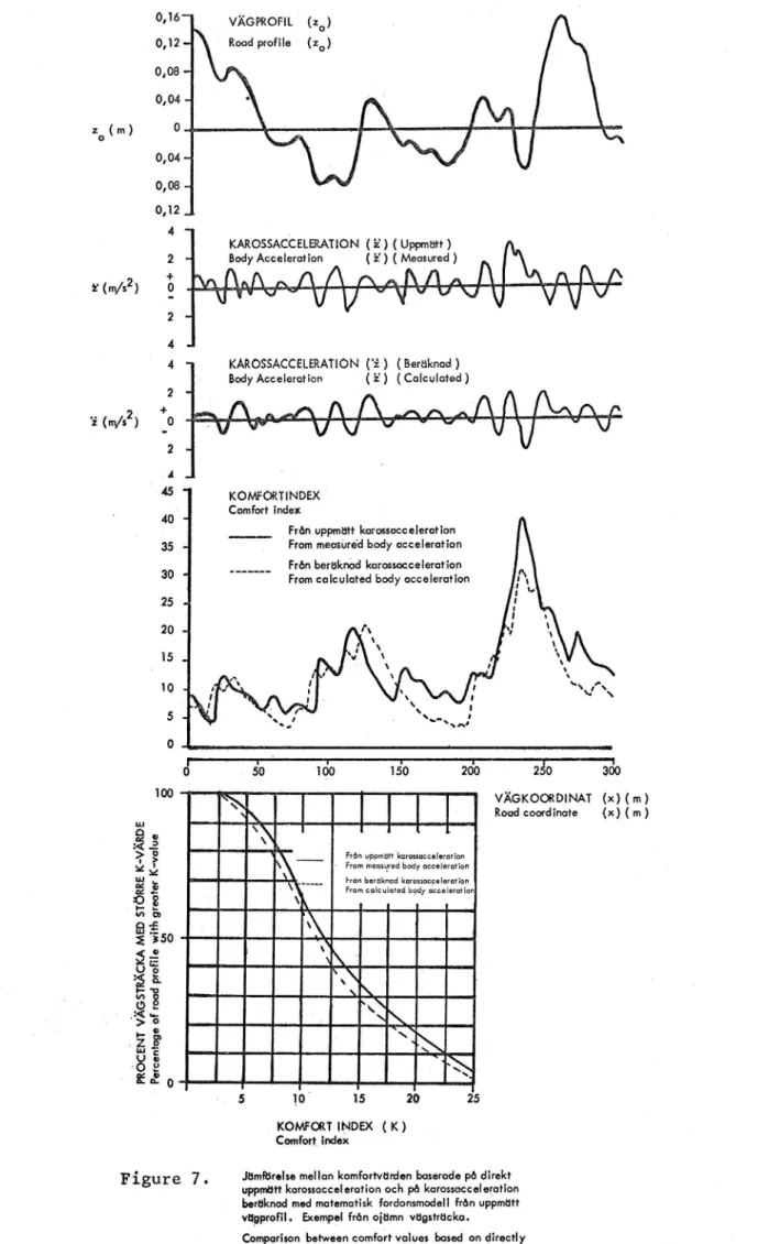
institute programmed with a model of a vehicle with the same data as the vehicle used in the measurements. The vehicle data are listed in table 4. In this way it was possible to compare comfort

parameters calculated by means of the vehicle model with the same parameters calculated from the acceleration record of DFl. The real vehicle and the model could thus be compared. Figures 7 and 8 show the results from the most even and most uneven sections

and illustrate the good agreement between the model and the

vehicle.

From the curves showing the comfort index and road holding index as a function of time (or length of road travelled) cumulative distribution curves have been computed. As a characteristic of the rOad section the median of this distribution curve was chosen

for cemfort index, whereas the road holding index was represented

-'by its first decile. These parameters were chosen because they gave the best agreement with subjective rating. The impact factor" was calculated on the basis of the first decile as explained above. ' Correlation coefficients between these parameters and the subjec

'tive rating were calculated assuming both linear and non linear

regression. The non~linear regressions gave the best correlation ' as shown in table 3.

Results from measurements with the CHLOE meter- .- ~ p... . a... u w o- m. - m u m wu m - . - .

The results of the measurements with the CHLOE meter on the 23

.test sections are shown in figure 9 as a relation between the RMS slope and the subjective rating. The curve calculated from

the AASHO PSI formula is also drawn as well as the TRAC curve. The lack of fit of the PSI curve may partly be due to the fact that the computation made here was based upon the CHLOE readings

only and not rutting, cracking etc.

A few points in the diagram have practically the same slope vari ance but differ considerably in rating. The corresponding sections

are number 5, 12, 15 and 18. These numbers are indicated in the

diagram. For a closer analysis Of these sections some other

para-meters were computed from the CHLOE data. These parapara-meters are the curvature, the jerk factor and the mean wave length. They were

computed in the following way.

The curvature was computed from the second derivative of the raod

profile, i.e. the differences between consecutive readings from the CHLOE meter. Division by the interval length (15 cm) of the difference between two consecutive readings (slopes = first deriva~ tives) gives second derivatives. At small slopes the second deriva ' tive is a goOd approximation of the curvature or the inverted

radius of curvature. The mean slope and mean curvature of a road section of the length measured here is normally.negligible in comparison to individual slopes and slope differences. The curva~ ture (like the slope) is therefore represented by the standard deviation around the mean, the RMS curvature. It may be difficult to visualize this measure of curvature, which is not the same as the overall curvature of the road section, this being represented

by the mean. The RMS curvature can be assumed to represent the occurrence of short segments of large curvature along the section

measured.

It is sometimes custumary to use the change of slope of a road surface as a measure of unevenness. This is for instance used in

detection of frost damage. Since curvature as defined here is

determined by changes in slope from one point to the next this measure of curvature may be a useful technique in replacing the

manual slope difference measurement used in such frost damage

characterization. The RMS curvature is given in units of inverse

kilometers.

The jerk factor is directly related to the third derivative of the longitudinal profile. When the human body is subjected to acceleration it subconsciously adjusts itself to the state of acceleration in order to compensate for the forces arising from

the acceleration. When the acceleration suddenly changes the body

registers the change in acceleration rather than the acceleration itself. This can be observed when a railway train stops after quite a gentle deceleration. Acceleration in the vertical direc-tion of an object moving along a road surface is at a given speed proportional to the second derivative of the road profile, and

the change in acceleration is therefore proportional to the third derivative of the profile. This quantity is therefore often

referred to as jerk. The root mean square of the third derivative of the road profile has therefore been denominated "jerk factor in the present work. Since the jerk factor is used only for comparison between different road sections no appropriate scale factor was included in the computer program. If the figures

given in the accompanying tables are multiplied by the factor 0.131 the third derivative will be obtained in rational units i.e. in-verse square meters. The jerk factor was like other similar para

meters calculated as the RMS of the third derivative, the mean

again being negligibly small in comparison to the RMS value.

fThe mean wave length was determined from Fourier.analysis of the

profile data. The CHLOE readings are prOportional to the deriva-tive of the profile, but by a slight modification of the library routine for Fourier analysis the spectrum of the profile itself can be computed directly from slope readings.

In Fourier analysis of a road profile this profile is decomposed into a series of sine shaped profiles of different frequency, amplitude and phase shift, i.e. a horizontal shift.of the nodes of the sine profiles. In the analysis the different sine shaped profiles are characterized by their wave length being equal to the length of the road section, in the present work 300 meters. The next wave length is half of this i.e. 150 meters, the next' 100 meters etc. In the present analysis 300 terms were computed, which means that the shortest wave length is l m. It often

happens in analysis of this kind that some property of the mea-suring object changes systematically with the length coordinate, and this results in an unproportionately high value of the compo

nents having the longest wave lengths, and the contributions from low wave length components of greater interest are obscurred. Two

Russian researchers, Skobelev and Filina (4), suggested that this

complication can be compensated for by analysing the deviations-of the prdeviations-ofile from its regression line. This technique was used

11.

here and resulted in a considerable reduction of the long wave length contributions. In the analysis components in the interval

1 ~ 10 m were recorded (components number 30 to 300). In this interval the mean wave length was computed by the formula

Lm=§§£

EA

A being the amplitude and L the.wave length of each component. It may not be easy to Visualize the meaning of Lm, but in

general a large value corresponds to extended "bumps" whereas a

small value illustrates irregularities close to rugosity.

In table 1 the curvature is listed in the fourth column, the fifth and sixth colums giving the jerk factor and the mean wave length \of some selected sections. It is seen in figure 9 that the RMS

slope of sections 5, 15, 18 and 20 ranges between 2.51 and 2.96,

whereas the rating varies from-1.65 to 3.32. This suggests the RMS slope to be a rather poor criterion of ridability. Sections 5 and 18 have a jerk factor of 3.49 and 2.45 respectively, whereas the mean wave length of both is 5.3. This suggests that the reason for the rating difference be the difference in jerk factor. The curvature of section 5 is 37 as against only 22 for section 18.

The higher frequency of occurrence of small curvature segments

in section 5 could have given the motorists an impression of higher bumpiness.

It seems contradictory that section 5 having the larger curvature of the two on the same time exhibits an equal mean wave length.

If small curvature segments are more frquent the mean wave length

should be smaller. In general, however an exceptionally large

mean, especially if based upon squares of components, may be a result of the occurrence of a small number of exceptionally large values rather than an exceptionally large number of moderately

large values, since the value itself is squared but not its freque

ency of occurrence in computation of the RMS.

12.

Section 20 was rated inferior to section 18, whereas both the jerk factor and the curvature of section 20 are considerably

less then those of section 18. The mean wave lengths are rather

close and similar to that of section 5. The spectrum of section

5 is on the other hand less "white" than those of sections 18

and 20. Several computed parameters are contradictory to rating

in this comparison.

.Obviously there are cases where the relation between driver's

experience and computed parameters is not simple. It should be

remembered that the sections just discussed had practically the same slope variance.

The cost of computation of second and third derivatives is only marginal. Fourier analysis is however rather expensive, even if advanced and well establiShed techique is available. Although not time consuming (one or two minutes per Fourier analysis, if the data are stored in an appropriate memory), the analysis engages the central processing unit of the computer quite considerably, and the cost of one single analysis has been 100 200 Swdish.

crowns ($ 25 w 50).

It should be remembered that the longitudinal profile is not alone responsible for the impression of unevenness. Between the driver and the road surface there is a vehicle, on which large costs have been spent on neutralizing the impression of unevenness. In

the parameters computed from DFl records these very properties

have been included, but only those of one particular vehicle. Comparison between CHLOE data and DFl parameters

cu w - -.~ ~ m .u-an a. - - wan v - c... - unnu .- _ u... - u o

Parameters derived from the CHLOE readings made on sections 1 23 are listed in table 1 and the DFl parameters (sections 1 r 22) are listed in table 2. The first column in each table gives the

section number.

13.

It can be observed that the relative range of variation of the different parameters is quite different. Road holding index and impact factor vary 6 and 12% respectively, comfort index varies

by a factor larger than 8 and the RMS slope by a factor 4 1/2. The first two factors also show the same value with several

sec-tions, and therefore ranking of sections with respect to these parameters was not possible.

The relation between subjective rating and the different computed parameters Was studied by calculation of the correlation

coeffici-ents. These correlation coefficients are liSted in table 3. The

coefficients are based upon individual ratings and not mean ratings. The first column gives correlation coefficients assuming linear relationship. These coefficients are in the interVal 0.5 ~ 0.7. A non linear approach of the form

rating = A + B - log (parameter + C)

can by proper selection of the constant C give a better fit.

-The corresponding correlation coefficients are listed in column 2 of the table. The.range is now narrower, but still RMS slope gives the best fit.

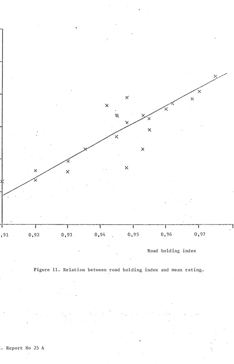
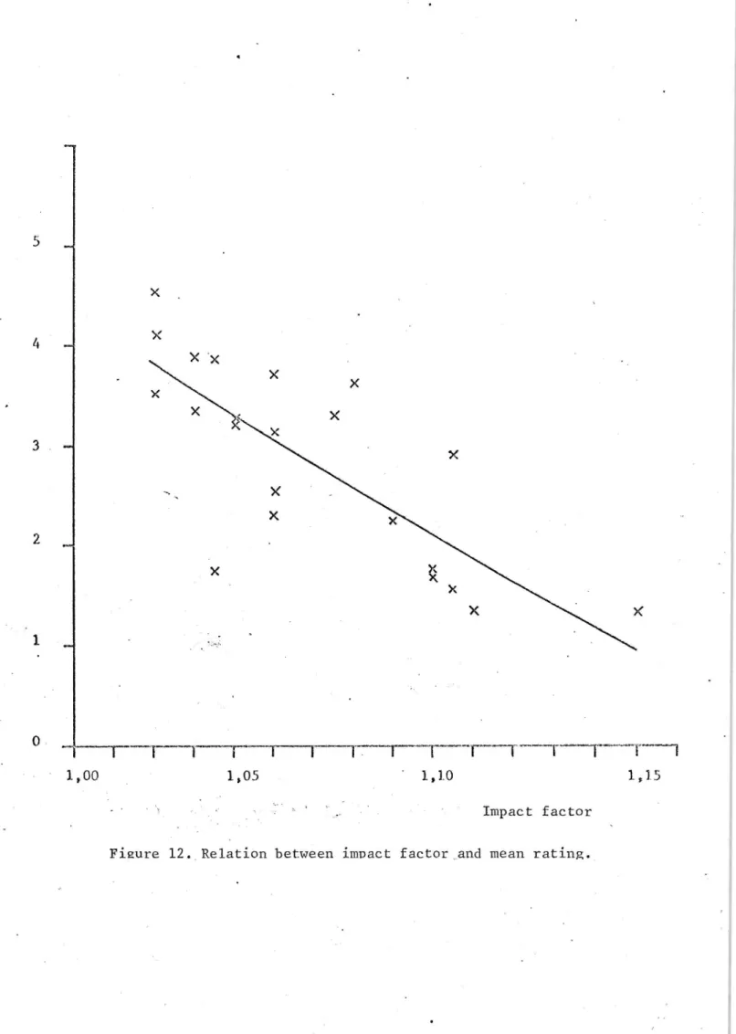
In the diagrams shown in figures 10 12 mean rating is plotted against comfort index, road holding index and impact factor. The diagrams also show the curve of best fit according to table 3. The smallest variance about regression is shown by the road holding index, Which also has the highest correlation coefficient. Of the parameters calculated the comfort index Was expected to give the closest relation with rating. This deviation from expectation I

.may partly be due to the fact that only one vehicle was used in

the computation, while ten different vehicle makes were used in

the subjective test. This may also eXplain why the only parameter which is a pure road parameter, the RMS slope, gave the best

correlation with rating.1

'If the different sections tested are ranked according to in

creasing mean rating and then rearranged according to the different parameters, the smallest number of permutations required for this_

rearrangement can be taken as a measure of the deviation between

subjective rating and rating on other basis. In this way the \ following number of required permutations are found.

14.

Parameter RMS slope Road holding Comfort Impact index index factor

Number of 25 37 32 36

permutations

The difference between the different parameters in this respect is not drastical, but again the RMS slope gives the least devia-tion from subjective rating, whereas comfort index gives the best agreement of the other three, which complies with expectation. The subjective visual and auditive impressions of the road and the vehicle travelling on it may have influenced the rating in the experiment. For an investigation of these factors a closer \look at the sections could have been helpful. For the present

(1973) practically all the sections are however resurfaced.

A direct comparison between the profiles recorded by means of the

two measuring systems is not feasible, since this requires profiling

along exactly the same track. Calculation of parameters based upon

vehicle dynamics and CHLOE readings was not feasible either, since this would have required tape records of the CHLOE data. Attempts have been made to calculate the RMS slope from the DFl tapes.

These however appeared to have a superimposed high frequency

spurious signal, which on differentiation dominated the tape output and little difference was found between the different sections. The only comparison feasible in the present investiga-tion was therefore the Fourier analysis. The results from sec-tions 18, 19, 21 and 22 are shown in figure 13. The spectra have quite a dispersion which is typical for spectra of stochastic variables. The spectra points of the two measuring systems however

show quite a reasonable agreement, and no pronounced difference

between the two systems can be read from the diagrams. Further

refinement of the data logging system of DFl will make it useful for calculation of the various RMS values computed from CHLOE readings in this report. Vice versa, the computation of parameters

15.

based upon vehicle dynamics from CHLOE readings is a matter of providing the appropriate computer soft ware.

Purposes of evenness measurements

Measurement of road surface evenness has at least two different purposes. One is production control, i.e. follow up of the paver

and roller action. The other is follow up of the state of the road during its life time, i.e. changes due to wear, rutting frost action etc. In conjunction with the AASHO test the corre-sponding state function was denominated serviceability, and

serviceability may be a useful indication of the life time and of the length of the repair cycle.

\For the first purpose the mechanized towed straighedge is used as a routine in Sweden. The degree of mechanization is determined

by economical rather than technical factors. The rules of

accep-tance are based upon this instrument; which in its most automized form is marketed for 20 000 Sw. crowns. The instrument has the main disadvantage that the length of the measuring base is deter mined by the measuring object and varies all the time during measure-, ment. The result of the measurement is therefore tied to the

design of the instrument. Since the instrument is well established, change to other instrumentation is not feasible, even if the two measuring systems described in this report will be able to give results which are independent of the.instrument.

For the second purpoSe, follow-up of the serviceability of the road, the two instruments described in this report are applicable.

The CHLOE meter was developed for this very purpose. For the choice of road characteristic there are several parameters which

can be derived from the original readings.

Comparison between the two measuring systems

The CHLOE meter is electrically and mechanically simple but has a very limited velocity (5 km/h). Its production capacity is there-fore low and it is a severe obstacle in the traffic, especially on motorways. DFl on the other hand can be run at normal speed and does not disturb the traffic rythm. With the present data processing routine used at this institute the data processing is tedious and costly.

16.

If interest in serviceability measurement arises among road authorities it would be practical if the existing equipment used for production control could be used. The measuring capacity of this equipment is however too low. DFl has a high measuring capa city but its purchasing price is high. The last known quotation of the GM instrument in USA is 50 000 U.S. dollars. The CHLOE meter of this institute was purchased in 1963 from the U- S. at

a cost of 50 000 Sw or (more than 10 000 U.S. dollars). In cost

comparison it should be noted that the GM meter is a vehicle in itself, whereas the CHLOE meter requires a towing vehicle._

In cost comparison the higher measuring capacity of DFl has to be balanced against the lower purchasing cost of CHLOE. In operating costs the data processing cost has to be included, which is among other things determined by the choice of parameter. It should be

observed that at certain times the demand of measuring capacity can be very large during short intervals, e.g. the thaw period. This increased demand favorizes systems having high measuring capacity.

In research the situation is different from that of regular road operation. The demand is more irregular and more difficult to prognostisize than in regular road operation. Sometimes a high measuring capacity is advantageous, and sometimes a towed

vehicle gives a greater flexibility in the disposal of measuring vehicles. The same vehicle can then be used for several measuring purposes. The CHLOE meter of this institute cannot according to Swedish traffic security regulations be towed at a higher speed than 20 km/h and must therefore be transported in the towing vehicle

also to rather closely located places.

REFERENCES

1. Lehtinen, E: "On the evenness of Finnish road surfaces as related to traffic engineering and road construction . Statens tekniska forskningsanstalt, Publication 159, Helsingfors 1970. (In Finnish with summary in English).

2. Kelly, W: "GMR road profilometer - a method for measuring road

profile , Highway Research Record, no 1, 1966.

3. Carey, W, Huckins, H and Leathers, R: "Slope variance as a measure of roughness and the CHLOE meter . Highway Research Board Special

report 73, 1962, p 132 135.

4. Skobelev, A and Filina, G: "Application de l'analyse de correlations spectrales a l'appreciation de l'uni des chausses . Laboratoire central des ponts et chaussées, Service de Documentation, Traduction

71 T 13 mars 1971. Translated from: Trudy Sojuzdornii, URSS, 1968,

no 19, p 113 119.

5. Mitschke, M: Beitrag zur Untersuchung der Fahrzeugschwingungen (Theori und Versuch), Deutsche Kraftfahrtforschung und Strassen-verkehrstechnik, Heft 157, 1962.

6. Andersson, 0: Test runs for determination of serviceability from longitudinal profiles. SVI Internrapport no 16, 1971. (In Swedish). 7. Sinha, B: Influence of road unevenness on road holding and ride

comfort. Inst for maskinelement, KTH Stockholm, Rapport no 1, 1972.

8. Andersson, 0: "On the analysis of longitudinal surface profiles by means of slope measuring profilometers", XIVth World congress

-- Prague 1971, Question IV:20, p 10.

SUMMARY OF RESULTS FROM ROAD RATING AND PARAMETERS DERIVED TABLE 1

-FROM THE CHLOE METER.

Section Mean rating RMS slope RMS curvature Jerk factor Mean wave

nr millira" inverse km length

dians 1 3,88 2,06 15,6 2 3,38 1,96 13,3 3 3,11 2,48 14,5 4 3,63 2,05 15,9 5 1,65 2,51 37,0 3,49 5,3 6' 1,37 5,66 32,3 7 1,32- 6,02 38,5 8 4,55 1,45. 10,9 9 4,10 1,54 11,4 10 2,27 4,74 ~32,2

11

2,57

4,10

28,6-12 '

3,35

2,49

14,3

13 1,88 5,82 38,5 14 1,75 6,42 43,5 15 2,92 2,83 14,3 1,25 4,2 16 3,73 1,96 15,4 17 3,84 1,72 13,7 18 3,32 2,82 22,2 2,45 5,3 19 1,59 4,81 17,5 1,46 5,8 _ 20 2,33 2,96 11,6 0,97 4,9 21 3,22 2,42 12,5 1,21 4,9 22 3,53 1,90 11,5 0,99 6,3 23 2,64 2,63 43,5 w EI, Report No 25 A

TABLE 2

DATA DERIVED'FROM MEASUREMENTS MADE WITH. DFl.

riwww 1_

Seg§ion Comfort index Road holding index Impact factor Mean rating

1 5 0,948 1,03 0 3,88 2 5 945 .03 0 3,38 3 5 948 05 0 3,11 4 4 942 07 0 3,63 5 12 920 09 0 1,65 6 15 920 10 0 1,37 7 17 910 14 0 1,32

8

2

975

'02 0

4,55

9 3 970 02-0 4,10 10 10 935 08 0 2,27 11 7 945 05 0 2,57 12 5 953 04.0 3,35 13 _ 6 930 C9 0 1,88 14 7 948 O3 5 1,75 15 13,5 955 O9 5 2,92 16 6 962 05 0 3,73 17 4 968 03 5 3,84 18 10 I 945 06 5 3,52 19 15,5 930 O9 5 1,54 20 8,5 953 05 0 2,33 21 8 955 04 0 3,22 22 3 960 02 0 3,53

VTI. Report No 25 A.

TABLE 3

CORRALATION BETWEEN INDIVIDUAL RATINGS AND DIFFERENT PROFILE

CHARACTERISTICS.

Characteristic 'Correlation coefficient with individual

rating

Linear relation Logarithmic relation

RMS slope -O,70lS V O,7338

Impact factor ~0,567l ~O,6377

Road holding index +O,6384 ' +O,7299

Comfort index ~O,6415 ~O,6577

Table 4. Vehicle data used for the calculation of K, R and P.

Vehicle ~ DFl 1963 Model, Rambler Ambassador (stationwagon)

Description Designation Dimension ' Data

Mass of the lower portion of the driver mpg kg 25

.Mass of the upper portion of the driver mF1 kg 30

Mass of the vehicle body m kg 1 800

Mass of the front axle mh kg 80

f

Mass of the rear axle mh kg 200

b

Moment of inertia of vehicle body around_ J kg m2 4 000

y axis ' y

. . * -_, 2 2

Moment of inertia of mF2 around mF1 S mF2 a kg m 6,25.

Spring constant of spring located KH .N/m 5 000 nearback of the driver

Spring constant of spring located KS N/m 7 000 'at the heap of the driver '

Spring constant of front and rear K3=K4 N/m 42 000 suspension springs

Spring constant of front tyre K1 N/m 600 000

Spring Constant of rear tyre K2, N/m - 600 000

Damping constant of seat damper (Horizontal) CH Ns/m 600

Damping constant of seat damper (Vertical) CS Ns/m 1 000'

Damping constant for front shock absorber C3 Ns/m '5 000

Damping constant for rear shock absorber 04 Ns/m 5 000

I Damping constant for front tyre_ C1 Ns/m lOO

Damping constant for rear tyre C2 Ns/m 100

Distance between CG and front axle f 'm 1,46

Distance between CG and rear axle b m 1,38.

Wheel base l=(f+b) m 2,84

Horizontal distance between CG and mF n m 0,2 2

Vertical distance between CC and InF I d m 0,5

I 2

Distance between H

I

31

and

mpz

, a m 0 5

Static axle load (rear) Phb (stat) N 11 200

Static axle load (front) P (stat) N 9 600

TI . R e p o r t N o 25 A .4

N

_i

_§

i' Al .. 'l .A -k -uwd wut -é' :_ 3" Z I aTape ingcorde.

a

7

u.-¢.A Road profile

r

If ... '.. ' : '6 . . ' Muff"; ux h,'...A.W .4 2 ... f .r -' . t v .«'

gmgq . rm

q -VA )#)_O O"»§I X.(§V,. (5:91. '

AuSmitch nlate board lIIIlllIllIIIIIITTIILIVIHIII 7 Roller contact Meaguring wheel _

._ ?iv0téng 29int

ReferenCe line Slgpe

Figure 3. Working principle df the CHLOE meter.

__ V .~_ .. -. -a.»-..

IO

1,0 v

V ER TICA L A C C E L E R A T I O N ,f Ma xi mum va lue u~ ! RM S va lue leg- 0 1

q,3o,5 1

2

5

10 2o

50 100

'FREQUENCY

(Hz)

Figure 5; Relation between frequency and vertical acceleration

at different values of K according to VDI recommendation

2057.

-;

V /\

L: .

5,3 stat

'

C) h: h: '4 u:

E

TIME [fjsec

g

/\

Z

L...

'I Q

3 P

53.1 5fo m P'

E

O ' TIME [fj'ge c 4. ' T. ' I . . [R P .o . 1 Road-hold1ng index\ ) 2 5 1 P :: f j $th 0 h P SP were E stat

I Figure 6. Definition of the Road holding index (R).

0:16

VKGPROFIL (2°)

O ,l2- 'Roadprofile (zo)

zolm)

2 (m/sz)

KAROSSACCELERATION (

Body Acceleration ( 'z') (Calculated)l( Beraknad )

'z'('m/52) +0

2 A A 45 1 KOMFORTINDEX 40' _ Comfort index

Fran uppmdtt karossaccelerat ion 35 .- t From measbre'd body acceleration

30 _______ Fran beraknad karossacceleration

From calculated body acceleration

o

' . so

100

150

260 -

230

360

VKGKOORDINAT (x) (m) Road coordinate (x) ( m )

Fran uppmdrt .karossacceleration

~ From measured body accelerat ion

Fran beraknad karossacceleration From calculated body ~accelerat

U! Q PR OC EN T VK GS TR KC KA ME D sr oR RE KV XR DE Pe rc en ta ge Of ro ad pr of il e wut h gr ea te r K-va lue O 5 10' 15 20 . KOMFORT INDEX ( K) Comfort~ index

Figure 7 . JdmiBrelsemellan komfortvdrden baserade pa direkt

uppmtttt karossacceleration och pa karossacceleration berttknad med matematisk -fordon smodell fran uppmdtt

vdgprofil. Exempel fran oidmn vdgstrdcka.

Comparison between comfort values based on directly

measured'bodyocceleration and on bodyacceleration computed from measured road profile. Example from

a rough road.

vklopkom (2.0)

Rood profile

KAROSS ACCELERATEON ('2') ( Uppmti rt)

Body Accelero on

('2') ( Measured )

_, ';-J . ~ ,4 x. WW; _.,-;x,,_wl my vb-.1 ." :..;b Aat,avidit $gll ir ._:

KAROSSACCELERATION. ( 'z') '(Ber'dknod )

Body Accelero on (35) (Calculated )

.. Me. H :5! 73",: v-~ at", .--~-w,. ~ ;,~lbf,-.u ;_ y e. I WJ'N? v i n- - ow}; v."

FriSn uppmo' korossocceferofian

From measured body acceleration g ____ M Frcm beriiknod kcrossocoe Iercmon i from coicuioted body acceleg'elthionv '

noex we; ~-~mw~- , ' > 7 a; a» ,1, w .1, t 3. » r'H. o '

0

5 i 5

50

100

150

200

2"!)

300

0/

vAoKooRmNAT

()4)

°

'

Rood coordinofe

(x)

E

100

-.

~

~

A

a

E _ 5

E E H E

§ 2 , Frénupom ot? koroesoooeiero on

mi: - From meowred body oooeiem on

'!

. i . .

g WW Frc'm ber oknod komssecceiermton

I

PR

OC

EN

T

VA

GS

TR

Ac

KA

M

ED

-S

YC

RR

E

K-vi

sl

ao

s

- From coéculofed body oooeiero on .

V . 0! O

Pe

rc

en

ta

ge

of

ro

ad

pr

of

il

er

wi

fh

gr

eo

fe

r

K-va

iue

o"

K t~i

o

'5

IO

15

20

25

KOMFORTINDEX. (K)

Comfort index

Figure 8, Jtimfo relse rheHon kom orfvo rden boserode pé direkt

hppm i korossoccelerotion Ooh pi: karossoccelerc on

bero knod med mofemo sk fordonsmodeH fron uppmd rt

v gprofil. Exempe! fré m itimn v o gs fr

dcko-Comparison befWeen comfort values based on direEHy

measured bodyoccelero on and on bodyacceierofion

computed from measured road profile. Example from

\

a smooth road.

'

2%. M _I

T RQQE;/ _X

I

I

.1

_

I

I4

'1

E

2

3

A

5

6

EMS slope, milliradians I

'FFigpre 9. Relation between RMS slope and subjeetive and calculated 5 rating.

!

3, ....

2 m

1- a;

0

I

I

1

l

I

I

I .I

i

l

l

1

1

:

rm :

0

5

10

15

Comfort index £\"

Figure 10. Relation between comfort index and mean rating.

and

% l . I I l. i l

\0 L0

0,91 .'

0,92

0,

0,94 .

0 95

0,96

0,97

Road holding index Figure 11. Relation between road holding index and mean rating.

mi 5N X

4;.

x

3....

2M lm

0.

lililll.lllilii

1,00 ' 1,05 v 1510 1,15 Impact factor Figure 12. Relation between impact factor and mean rating._

SECTION 22 (3 ( G 9 . ... D a (2 U D[] 6 e 1:: _CE. (:2 _{D g [-12, e -01 e} . i (j K LI . I 4 ,

G

6 9 3 0 ( 2 c5919 c9 0010 0 cs

8

06.3630 C d

C

{ 1 1 1 I 1 1 1 3 1 I 1 I I I I l I I I I I I | 1 5 _{» FREQUENCY (Hz)}, 20 25 I I I I I I I I I A I I - ' ' I 25 1o 8 7 5 5 4 3 2 1,5 - 1,25 1 WAVELENGTH (m) ' SECTION 21 e a e [:1 _ 0 , a

G e

a 6D

0

3

0"

D

D p n

e

I

_{0* *1}

I ,

I

Q g»? <3. £30., 52,351.25 I3

i I I I 3 I I

8 e

I I 3

C" 8 a 1:1 5 (163 a":

i I 1 i 1 I , 1 1 5 1o _{FREQUENCY (Hz)}, 15 2o . 25 I I I I I I I I ' | I I I ' I I I 25 1o 5 4 3 2 1,5 1,25 1 ~ g,0% ' WAVE LENG TH (m) ' ea: _{SECTION I9} e ~ ee _{e e} 0 D D M G U u (:1 page 0 a e a $65 a e

a 8 £3

610 a

61:: @De @ 3 I 6" g c:

C -

<

I T I I r g I0 19 a 2 a . a, 1 e I 1 $3 g} (73 (I) Q [7:

I

'

-»

0 EREQUENCHHZ)

5

20

25

I

I II I I I |

'

I

'

I

'

'

I '

i

25 1o 5 4 3 2 1,5 1,25 1 _.. - WAVELENGTH (m) 6 SECTION I8 0 M [:1 a a i . U a . [3 - e , e as

_{e a 1:] D}

ea 1:1

_e

_e

1:1 [:1

_n

_{. 8}

_{. g}

.

₈

_e

9' e e ' I 9

6098886003'@

«19

8510093,:

1 1 1 1 I 1 1 *1 1 I 1 r 1 1 1 1 1 l 1 26 1 1 1 1 , I 5 10 FREQUENCY (Hz) 15 25 I I I I I I ' I I I . I ' > I 25 1o 5 4 3 2 . 1,5 1,25 1 . WAVELENGTH (m) _ I

Figure 13. Comparison between road profile amplitudes at different wavelengths obtained by means of Fodrier analysis for road profiles measured with

DFl and CHLOE. o = DFl o = CHLOE. The frequencies given in the figure

. I refer to a speed of 25 m/s.