2005:07 An Assessment of SKB's Performance Assessment Calculations in the Interim Main Report for the Safety Assessment SR-Can

(1)

SKI Report 2005:07

Research

An Assessment of SKB's Performance

Assessment Calculations in the Interim Main

Report for the Safety Assessment SR-Can

Philip Maul

Peter Robinson

March 2005

(2)

(3)

SKI- perspective

Background

The Swedish Nuclear Fuel and Waste Management Co, SKB, has the intention to submit a licence application for building a final repository for the spent nuclear fuel at the end of year 2008. In preparation for the application SKB has published an interim main report of the safety assessment SR-Can, to demonstrate the methodology for safety assessment. The methodology will be used in the complete safety assessment SR-site, that is to support the licence application in 2008.

Purpose of the project

The objective of this project is to reproduce SKB's Performance Assessment (PA) calculations given in the interim SR-Can assessment using the AMBER modelling package. This has previously proved to be the only effective way of obtaining a detailed understanding of SKB's assessments, and should provide essential information for the future review process. Evaluations are also performed of the background information provided in the Interim SR-Can Report that is relevant to the PA calculations.

Results

Probabilistic calculations are done with AMBER modelling package, with selected use of sampled parameters from SR-Can have provided very similar results to those in the Interim Report for both the Base case and the variant where all canisters are assumed to fail simultaneously. This in spite of the fact that SKB’s SR-Can probabilistic

calculations use output from hydrogeological calculations, and only summary data have been presented in the Interim Report. This means that a full reproduction of the SR-Can probabilistic calculations was not possible.

There remain uncertainties over how SKB have modelled the U-238 decay chain. AMBER calculations that assume the daughters of Ra-226 are mobile (not sorbed) in the near field and geosphere give calculated dose rates that are typically an order of magnitude higher than obtained under the assumption that they have similar transport properties to the parent.

There remain uncertainties over the details of how SKB have modelled the transport resistance at the buffer-fracture interface. Fixed values for the lumped transport resistance parameters were employed in the AMBER calculations reported here.

Project information

Responsible at SKI has been Benny Sundström. SKI reference: 14.9-040145

(4)

(5)

Research

An Assessment of SKB's Performance

Assessment Calculations in the Interim Main

Report for the Safety Assessment SR-Can

Philip Maul

Peter Robinson

Quintessa Limited

Dalton House

Newtown Road

Henley-on-Thames

Oxfordshire RG9 1HG

United Kingdom

March 2005

SKI Report 2005:07

(6)

(7)

Summary

SKB have published their Interim Main Report of the safety assessment SR-Can, which is intended to establish the framework for what will be submitted in 2006 in support of a licence application for construction of the spent fuel encapsulation plant. This follows on from the SR-Can Planning Document published in 2003. The purpose of the Interim Report is stated to be to demonstrate the methodology that will be used for safety assessment.

The present report evaluates the information provided in the Interim SR-Can Report that is relevant to the Performance Assessment (PA) calculations that SKB intend to

undertake, using independent calculations to facilitate this process.

SKB consider that the primary safety function is to isolate completely the fuel within the canisters over the entire assessment period. Should a canister be damaged, the secondary safety function is to ensure that any release is retarded and dispersed sufficiently to ensure that concentrations levels in the accessible environment cannot cause unacceptable consequences.

In this report PA calculations are considered to include both a high-level representation of the evolution of the system (relevant to the primary safety function), and any

subsequent radionuclide transport (relevant to the secondary safety function). The main conclusions drawn are:

1. The effects of climate evolution on engineered barriers have not been analysed in detail in the Interim Report, and this limits the usefulness of the preliminary calculations that have been undertaken.

2. A key aspect of SKB's approach is the use of an integrated near-field evolution model. The information provided on this model demonstrates its capability efficiently to reproduce calculations from individual process models, but insufficient information is given at the present time to justify statements about interactions between processes. In particular it is assumed that relatively short-term thermal and resaturation processes do not affect the properties of the buffer and its longer-term performance.

3. The underlying methods for considering radionuclide transport are little changed from SR 97, although useful improvements have been made in some areas. The approach taken means that additional calculations are needed to address issues related to the evolution of the system with time. Whether the overall

methodology will enable a comprehensive assessment to be undertaken in practice can only be judged when the full SR-Can assessment is available. 4. The documentation of the models used in PA calculations often relies on

(8)

5. The consideration of conceptual uncertainties in the supporting Process Report is restricted to the buffer. This restriction greatly limits the usefulness of the Process Report in providing information on the overall methodology. For example, it is not clear whether the approach taken for the buffer will be satisfactory for addressing conceptual model uncertainties in the geosphere. 6. SKB have not presented any deterministic PA calculations. Without these it is

often difficult to understand fully the probabilistic calculations that are presented, although independent AMBER calculations have been able to

reproduce the key features of these calculations. It is suggested that deterministic calculations should be part of SR-Can safety assessment.

7. It has been possible to reproduce the key features of the interim SR-Can probabilistic calculations with AMBER, although there remain uncertainties deriving from the way that SKB have modelled the U-238 decay chain in different parts of the system.

8. A full reproduction of the interim SR-Can calculations was not possible because only summary data from hydrogeological calculations are presented. It is

suggested that in the SR-Can safety assessment sufficient information should be provided to enable PA calculations to be fully reproduced.

9. SKB's preliminary calculations indicate that safety criteria are likely to be met by a comfortable margin even if a large fraction of the canisters fail. The geosphere plays only a minor role in the retardation function. This assertion depends on a number of assumptions, and the independent AMBER calculations show that different assumptions could mean that the safety criteria would be exceeded in this extreme case.

(9)

1 Introduction

SKB have published their Interim Main Report of the safety assessment SR-Can, which is intended to establish the framework for what will be submitted in 2006 in support of a licence application for construction of the spent fuel encapsulation plant (SKB, 2004a); this document is hereafter referred to as the Interim Report. It follows on from the SR Can Planning Document (SKB, 2003) that was reviewed by Maul (2003a); this is referred to as the Planning Document. The purpose of the Interim Report is stated to be to demonstrate the methodology for safety assessment.

The objective of SR-Can is stated to be to investigate whether canisters of the envisaged type are suitable for disposal. The report aims to show how SKB plan to handle the SR-Can safety assessment in a way that meets the requirements of the regulations laid down by SKI and SSI. Example information is taken from the Forsmark site in several places. It is stated that the full assessment report structure will be similar to the structure of this interim report.

The present report evaluates the information provided in the Interim SR-Can Report that is relevant to the Performance Assessment (PA) calculations that SKB intend to

undertake, using independent calculations to facilitate this process.

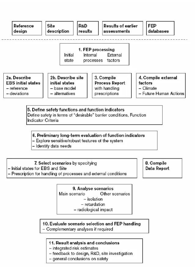
The Interim Report structure generally follows the overall methodology that is described. The methodology is broken down into 11 steps, as shown in Figure 1. In Table 1 a mapping is provided between the identified individual steps in the

methodology and their treatment in the Interim Report. There is not a simple one-to-one link between the methodology stages and the Interim Report sections.

SKB consider that the primary safety function of the disposal system is to isolate completely the fuel within the canisters over the entire assessment period. Should a canister be damaged, the secondary safety function is to ensure that any release is retarded and dispersed sufficiently to ensure that concentrations levels in the accessible environment cannot cause unacceptable consequences.

In this report PA calculations are considered to include both a high-level representation of the evolution of the system (relevant to the primary safety function), and any

subsequent radionuclide transport (relevant to the secondary safety function). The report is structured as follows:

• A discussion of SKB's overall methodology is given in Section 2 to give the background to the approach taken to PA calculations.

• Those parts of the Interim Report that are mainly concerned with evolution of the system and the primary safety function are discussed in Section 3. No independent calculations for system evolution have been undertaken at the present time.

(12)

• Independent radionuclide transport calculations, undertaken to gain further insight into the SKB calculations, are presented in Section 5.

• Finally, the main conclusions from the work are brought together in Section 6. The Interim Report refers to several related reports, including those on FEPs, processes, data and the initial state of the system (SKB 2004b, 2004c, 2004d and 2004e). These documents are also referred to in this report, but have not all been individually assessed.

(13)

(14)

Table 1: SKB Safety Assessment Methodology and the Interim Report Structure.

Methodology Step SKB Documentation Comments

1. FEP Processing FEP Report 2. Initial States Chapter 3 3. Process Report Chapter 5 4. EFEPs Chapter 4 5. Safety Functions and Function

Indicators

Chapter 6

6. Preliminary evaluation of function indicators

Chapter 7 Includes consideration of alternative ‘top level’ indicators that do not require detailed assumptions on the biosphere and human habits. 7. Scenario selection Chapter 8

8. Data selection Data report

9. Scenario analysis Chapters 11 and 12 Separation of the ‘isolation’ (chapter 11) and ‘retardation’ (chapter 12) functions 10. Additional scenarios -

11. Results and conclusions Chapter 13 Only expected content discussed at this stage

(15)

2 Overall Methodology

The Interim Main Report is based on the original KBS-3 concept with vertical

emplacement of waste canisters (KBS3-V). Reference is made to an alternative concept KBS3-H [Section 1.1.1], with horizontal emplacement of cylinders, and to Posiva’s safety assessment planned for 2007 of this concept. However, this date is after the application will be made for the encapsulation plant. It might be considered, at least in principle, that canisters suitable for KBS3-V might not be suitable for KBS3-H, and SKB's perspective on the safety and performance assessment implications of continuing to carry forward an alternative concept is therefore not clear.

2.1 Safety Functions

In Section 2.1 of the Interim Report it is reiterated that the primary safety function of the system is to isolate completely the fuel within the canisters over the entire

assessment period. Should a canister be damaged, the secondary safety function is to ensure that any release is retarded and dispersed sufficiently to ensure that

concentrations levels in the accessible environment cannot cause unacceptable consequences. The safety principles are expanded in Section 2.6.1.

2.2 Function Indicators

Based on the Process Report (SKB, 2004c), a number of preliminary criteria have been defined. The definition of these function indicators is part of Stage 5 of the overall methodology, and these are addressed in Section 6 of the Interim Report.

SKB make it clear that satisfying these criteria does not necessarily mean that the requirements of the regulations will be met. These intermediate criteria are, however, useful in clarifying SKB’s views on how the engineered near-field should perform. The function indicators relate to the engineered near-field, groundwater chemistry and rock shear. This is consistent with the overall safety concept to isolate the spent fuel in the canisters for the whole period of the assessment.

An example of the chosen function indicators is the maintenance of a buffer density of greater than 1800 kg m-3_{to avoid microbial activity. In addition, if the density is greater}

than 1650 kg m-3 it is stated that fuel colloid transport will be prevented. Such criteria need to be reviewed by experts in the relevant technical areas; they are not addressed in the present report, which is concerned with more general PA issues.

Table 6-1 [Section 6.4.1] p128 gives a useful summary of system properties that contribute to retardation. The aim is to complement the dose/risk criterion with indicators that do not need detailed assumptions about the biosphere and/or human habits. Reference is made to EU projects and Finnish criteria, and a decision is taken to use the Finnish criteria for fluxes to the biosphere.

(16)

2.3 Internal Processes

This part of the overall methodology is addressed in Section 5 of the Interim Report. Section 5.1.2 states that all biosphere FEPs have been collected into a single category. A Biosphere Process report will be published. SKB's modelling hierarchy for the

biosphere is not currently clear and, until it is, it is going to be difficult to undertake a formal FEP analysis, or understand what their overall strategy in relation to biosphere uncertainties is. This issue is linked to the way that the biosphere is modelled separately from the rest of the system (see Section 2.4).

Process representations are considered in Section 5.2. Problems with process diagrams and interaction matrices are discussed – neither will have a central role in SR–Can. Instead tables giving the relationship between model parameters (variables) and processes are explained in Section 5.4 where an example table is given for the buffer. The overall approach is to document each process in detail in the Process Report, and map these processes onto model parameters; the approach has some common features with the AMF envisaged in the Site-94 study.

2.4 The Biosphere

It is stated [Section 2.8] that the biosphere is treated differently from the rest of the system. In the example calculations a constant temperate biosphere is considered with probabilistic EDF’s considered (as in SR97). It is not yet clear how SKB will handle a time varying biosphere [Section 2.8.3]. It is stated that a fully integrated time-dependent treatment of the biosphere is not contemplated because of the dominance of biosphere uncertainties and the more rapidly varying timescales.

SKB's arguments for essentially decoupling the biosphere have some validity, but if whole system modelling is not to be employed, there is the potential for problems of inconsistency between assumptions made in different parts of the system, particularly when sensitivity calculations are undertaken. Currently, the calculations presented in the Interim Report are based on simple scenario assumptions for environmental change, so it is not possible to examine SKB’s approach to dealing with such considerations. By employing a whole system model, SKI will be in a good position to investigate this possibility when SKB's full assessment is submitted.

2.5 Compilation of Data

It is stated [Section 2.7.1] that a new procedure has been introduced (although this has only been fully demonstrated for buffer migration data). Data now include information that is relevant to repository evolution (not just radionuclide migration). This is

consistent with the distinction between primary and secondary safety functions. The Data Report (SKB, 2004d) gives details of the advice given to experts on how uncertainties should be expressed and how correlations should be handled. It is not clear, however, how uncertainties arising from the use of detailed supporting-level calculations will be represented at the PA level.

(17)

2.6 Management of Uncertainties

SKB's classification of uncertainties [Section 2.11.1] into System Uncertainty, Conceptual Uncertainty and Data Uncertainty follows previous usage.

System Uncertainty is managed primarily using FEP analysis. The FEP report (SKB, 2004b) gives details of the FEP database that has been used, although it is stated that this is only an interim version. This FEP report has not been considered in detail in the present report.

It is stated that the handling of Conceptual Uncertainties is addressed in the Process Report (SKB, 2004c), although the present version of the process report only considers the buffer. This restriction greatly limits the usefulness of the Process Report in

providing information on the overall methodology. For example, it is not clear whether the approach taken for the buffer will be satisfactory for addressing conceptual model uncertainties in the geosphere.

2.7 Risk Calculations

In Section 2.2.12 arguments are given for the necessity to overestimate risk in situations where credit cannot be taken for some processes. Discussion of the consideration of the problem of risk dilution by comparing the ‘mean of the peaks’ with the ‘peak of the means’ is a sensible approach. The example calculations show that, because the system is so dispersive, risk dilution is not really a problem, and this is consistent with the conclusions drawn by Quintessa. However, in the full assessment the representation of the processes that contribute to the dispersive nature of the system (e.g., the slow release rate from the fuel and the transport resistance at the buffer-fracture interface) will need to be scrutinised.

(18)

(19)

3 System Evolution and the Primary Safety Function

3.1 Evaluation of Function Indicators

This part of the overall methodology is addressed in Section 7 of the Interim Report.

The bounding approach taken in the Planning Document is employed, considering two groundwater types: ‘saline ice front’ and ‘non-saline melting zone’ – no attempt is made to analyse climatic evolution as part of a time-dependent representation of system dynamics.

Our understanding of this stage in the overall methodology is that it is designed to demonstrate that the main function indicators can be met using robust arguments that don’t depend on detailed consideration of climatic evolution. This is consistent with the emphasis placed on the isolation safety function. This seems sensible provided the bounding assumptions can be demonstrated to be robust.

The main tool employed by SKB is the integrated near-field evolution model.

3.1.1 The Integrated Near-Field Evolution Model

This model is described by Hedin (2004), and the key features of the component models are given in Table 2.

As stated in the Interim Report, there is generally no simplification of the equations used in the detailed supporting-level codes, although bespoke, more rapid, solution methods have been employed.

The canister interior model is not needed in the evaluation of the function indicators as these are only concerned with the isolation safety function.

The short-term saturation of the buffer is not included in calculations, and it is stated that output from one model is generally not used as input to other models in the present version. The maintenance of an even bentonite swelling pressure during resaturation is questionable, especially given that water inflow to the engineered system is going to be inhomogeneous.

No real 'integrated' calculations are presented. It would appear that the present version of the code has made the solution of the different models more efficient, but hasn't yet been used to investigate model interactions in any detail.

(20)

Table 2: Components of the Integrated Near-Field Model.

Model Function Comments

Source-term Calculation of Radionuclide Inventories and the Heat Source

Heat output is approximated as a sum of exponentials. This approach has been used elsewhere and should not lead to any significant uncertainties in the calculations.

Thermal Calculation of temperatures throughout the system as a function of time.

The methods employed are well established and should not lead to any significant uncertainties in the

calculations. Rheology Calculation of the buffer

density and pressure as a function of time.

The buffer density is important in the specified function indicators. It is argued that the details of the initial resaturation period are not important.

Buffer Chemistry

Calculation of pH, pe (electric potential) and ion

concentrations as a function of time.

Takes the buffer to be uniformly mixed, but uses the same model equations as the more detailed supporting-level model.

Copper Corrosion

To calculate canister corrosion rates.

Uses transport resistances to calculate the transport of corrodants to the canister. Canister Interior To calculate water level and

pressure in the canister following canister failure.

Given the importance of this work to the overall safety case being made by SKB, this is an area where SKI needs to consider whether independent modelling work should be undertaken. In particular, such activity be would help to ensure that the scope of the PA encompasses the various levels of understanding necessary to assess compliance with regulatory requirements – especially with regard to demonstrating the primary safety function of the disposal system.

The canister corrosion model uses analytical expressions from Neretnieks (1979, 1986) for the transport resistance model at the buffer/fracture interface. Concerns have

previously been expressed (e.g. Maul 2003a) on the validity of this approach over the whole range of model parameter values. A discussion of the treatment of transport resistance at the buffer-fracture interface is given in Appendix A of this report.

3.1.2 Calculations for the Isolation Function

It is concluded in Section 7.2.2 that the canisters without defects will remain intact for the whole of the assessment period, provided that geochemical conditions remain stable, and that only 1 or 2 canisters are likely to fail in a million years due to weld defects.

(21)

It is further concluded [Section 7.2.3] that if oxygenated water reaches a canister it will still not fail for 400 000 years. Superficially this appears to be a surprising conclusion, and needs to be considered further in near field evolution modelling.

According to the analytical methods used in the canister corrosion model, the number of failed canisters caused by pyrite in the buffer is proportional to time and depends on: the pore water concentration limit of sulphide; the effective diffusivity of sulphide; and the concentration of pyrite in the buffer.

There is an assumption in the SKB document that during the (relatively early) thermal phase and during the period of resaturation, the buffer properties are not affected. However, the inhomogeneity of the resaturation process could possibly lead to effects on the buffer that might then affect the later evolution of the system.

Several of the safety arguments depend upon the maintenance of a high buffer density. Calculations undertaken with the rheology sub-model aim to demonstrate that these criteria will be met.

The buffer chemistry calculations assume a uniformly mixed buffer. This is probably an acceptable approximation, but this needs to be checked. The only way that the buffer chemistry calculations can be independently assessed by SKI would be to do undertake detailed calculations with a code such as RAIDEN, which has previously been

employed by Quintessa for SKI.

3.2 Mechanical and Hydro-Mechanical Issues

Because the primary safety concept depends upon maintaining the integrity of the canisters over very long timescales, any evolution of the system that could threaten this integrity is critical for the safety case. SKB previously stated [Planning Document Section 5.1.8] that coupled MH (mechanical-hydrogeological) models are currently under development, but it is not clear from the Interim Report what the status of this work is.

Mechanical and hydro-mechanical issues are considered separately in Section 10 of the Interim Report. It does not correspond to a stage in the overall methodology and links to other aspects of the safety assessment are not made clear. It is stated that all of the work presented is of a preliminary nature, and it is not evident how this topic will be reported in the structure of the Final SR-Can Assessment.

The possible effects of a fault intersecting a deposition hole are considered in Börgesson et al. (2004) using finite element calculations. This leads to the definition of a canister failure criterion of a rock displacement of 10 cm. SKB's analysis appears to be based on the assumption that movement along a horizontal shear is the most severe test for a vertically emplaced canister, but this may require further justification. This supporting document has not been considered in this report.

(22)

3.3 The Main Scenario

Chapter 11 of the Interim Report considers the evolution of the system. It is emphasised that the integrity of the barrier system and climate evolution have not yet been dealt with in detail, and this limits the scope of the example calculations that are presented. The focus is on canister integrity.

In many places the issues that need to be addressed are clearly presented, but only limited information is given on how this will be done.

Section 11.2.5 addresses the resaturation period. It is stated that this work is on-going and no single reference for the calculations presented is given. Variant calculations have been undertaken following the approach taken in SR 97. It is concluded that the buffer will saturate in at most a few hundred years (a few thousand in some ‘extreme’

calculations). It is argued that there are no adverse effects on performance due to partial saturation, with no corrosion taking place during this period. As noted in Section 3.1.2, it is not obvious that the properties of the buffer would not be affected by processes taking place in the resaturation period.

It is stated that chemical evolution calculations will be undertaken using PHREEQC, but little detail is provided. Reference is made to the integrated geochemical model for the near field described by Domènech et al. (2004), which is used to consider the chemical evolution of the buffer and backfill.

(23)

4 Radionuclide Transport and the Secondary Safety

Function

4.1 Inputs to the PA Calculations

4.1.1 Scenarios

SKB’s approach is influenced by the SKI regulations that refer to a main scenario, less likely scenarios (including the effects of damage to barriers as a result of human actions) and residual scenarios (including the effects on people from human intrusion). Alternative design options will be considered in variants to the main scenario. This will include alternative backfill materials, but no reference is made to the KBS3-H

possibility.

It is stated [Section 8.2.1] that at the present time it is not meaningful to differentiate between uncertainties analysed within variants to the main scenario and less probable scenarios. It is not clear if SKB anticipates that this will be done for the 2006 SR-Can assessment. Their argument that this doesn’t really matter is probably correct.

Section 8.3.1 gives examples of deviations from the reference initial state that will be used in residual scenario calculations.

4.1.2 Hydrogeology

This is considered in Section 9 of the Interim Report. It does not correspond to a stage in the overall methodology, but is presented as an introduction to the following sections. It is stated that in the full assessment this material will appear in supporting documents. CONNECTFLOW and Darcy Tools are used.

Regional modelling is undertaken to provide details of the time evolution of the flow and salinity fields. DFN models do not take salinity into account. It is stated [page 193] that in order to demonstrate the groundwater flow and transport methodology described in the Planning Document, nested models have been constructed on various scales. It is possible that the use of nested models could propagate errors down the scales.

This modelling work is described by Hartley et al. (2004), which was not available at the time that the Interim Report was published, although it has subsequently been made available on SKB's website. A mixture of continuous porous medium (CPM) and discrete fracture network (DFN) models are used in these calculations. Inputs to the PA calculations include: Qeq, the equivalent flow rate at the canister; Tw, the travel time in the geosphere; and the F factor used in geosphere transport calculations. Probability distributions are given for these quantities based on the original interpretation of Forsmark data and for a more recent, updated interpretation. There are potentially significant differences between the two sets of calculations for these quantities. For example, for the Q1 pathway where a fracture intersects the buffer the initial calculation

(24)

mean value for the parameter F for this pathway was 6×106_{y m}-1_{, and the updated value}

was 3×107_{y m}-1_.

In the Interim report it is correctly stated that these PA parameters are correlated, and this is taken into account in SKB's calculations. The way that probabilistic

hydrogeological calculations are fed into the SKB PA calculations is, however, unclear. Some particle tracks return to the surface within 100 years, but others take a much longer time to return to the sea. This explains why some of the calculations for Tw give a bimodal distribution.

4.1.3 The Geosphere-Biosphere Interface Zone

SKB’s treatment of the geosphere-biosphere interface is discussed in Section 9.3.3. A sensible approach appears to be taken, aiming to identify the relevant flux of near-surface water with which the emerging radionuclide flux will be mixed. More detailed surface hydrogeological modelling will be undertaken for the final assessment, although it is unclear how this fits into the overall model hierarchy within the decoupled system modelling.

In the earlier Planning Document [Section 5.2] reference was made to the problem of how best to represent the coupling between near-surface hydrogeology and deep groundwater flow. Reference was made to a report in preparation by Holmén and Forsman that the existing groundwater flow models can be used if a high resolution is applied close to the surface. This work appears not to be referred to in the Interim SR Can Report, so it is unclear what specific approach will be followed.

4.2 Analysis of Failed Canisters

This is undertaken in Chapter 12 of the Interim Report.

SKB are still not clear whether they will need to present calculations for alternative scenarios with canister failure: redox changes due to oxygenated glacial water and rock shear movements at a deposition hole. The starting point for the analysis is the

previously referred to calculation of an average of one canister failure in a million years from corrosion.

4.2.1 Transport from the Canister

Consideration is given to the possible evolution of the internal canister after failure, but it is concluded that no credit can be taken in the safety case for any radionuclide

containment after failure (previously there remained a resistance to transport even with a large hole in the canister). The justification is given [page 263] for a 1000 years delay followed by a progression to a zero transport resistance some time before 100 000 years. Sagar et al. (2005) have commented (Section 2.5 of their report) that further justification is needed for the parameterisation of the time delay before radionuclide releases

(25)

report. Clearly, however, the fuel dissolution rate is a key parameter in the overall determination of radionuclide release back to the biosphere from a failed canister. No consideration appears to be given in the Interim Report of the affect on fuel dissolution rate if oxygenated water reaches the canister.

4.2.2 Transport in the Buffer

The old COMP23 model is still used for near-field transport. A model validity document has yet to be produced for this code. In the earlier Planning Report it was stated that COMP23 has been developed to enable solubility limits and advective transport to be represented. It is not clear in which situations advective transport will need to be considered.

Equivalent flow rates for fractures are still input to the transport model. It is stated that these quantities are now calculated directly from the hydraulic model, which is stated to be an improvement over SR 97 (where generic assumptions were used). Reference is made to a 1998 report by Moreno and Gylling for the equivalent flow rate within the EDZ, although this is not included in the list of references for the Interim Report. The use of these equivalent flow rates is an example of where the SKB documentation has been difficult to follow and is sometimes contradictory; these concerns are discussed further in Appendix A.

The model validity document for COMP23 will be considered when it is available.

4.2.3 Transport in the Geosphere

As stated in Maul (2003a), there seems to be a proliferation of models referred to by SKB, and it is not always clear how and under what conditions the different models will be used within the safety assessment as a whole.

Some issues associated with transport modelling are discussed in Section 9.4 of the Interim Report, but it is not clear why this has been included in the hydrogeology section. It is stated that no changes have been made to the 1D approach discussed in the earlier Planning Document, so the limitations of this approach referred to in Maul (2003a) remain valid.

Elert et al. (2004) give the 'model validity document' for FARF31. This report contains nothing new, but sets out the reasoning for the continued use of a 1D approach, and details of the verification of the code.

A new modified version of FARF31 has been produced, FVARF, using the finite volume method (Vahlundand and Hermansson, 2004). The governing equations are not given in the Interim Report. In the Planning Document [Section 5.3], SKB referred to a finite volume based model using an integrated form of the governing equations with the system being discretised into a number of domains. It was stated that this model has been implemented in Matlab, but it is not clear if this model is the FVARF code referred

(26)

would be instructive to investigate whether the SKB calculations described in this report could be reproduced using a tool such AMBER.

In the Planning Document SKB also referred to a so-called ‘segmented FARF31’, in order to investigate the importance of properties changing along the flow path. This approach is needed if decay chains are to be treated properly when properties vary along the flow path, but no detailed information is provided, and this appears also not to be referred to in the Interim Report. Reference was also made in the Planning Document to the use of a modified version of FARF31 for the backfill, linked to a FARF31

calculation for the geosphere. It is not clear what has happened to this intention. It is stated that the rock transport resistance factors F are now calculated directly in the hydraulic model. A reduction factor of 10 is applied to allow for channelling, as justified in the Data Report.

Another detailed code that will be used is the channel network model CHAN3D which solves for both flow and particle tracking. In the Interim Report it is stated [page 193] that CHAN3D will be used to investigate the importance of transition between climate states because the main transport code cannot deal with this time dependency.

The Data Report gives details of the parameters needed by FARF31 and COMP23 and refers to supporting detailed calculations such as Hartley et al. (2004). The justification for these parameter values has not been evaluated in this report.

4.2.4 Transport in the Biosphere

The approach to biosphere modelling is stated to be more comprehensive than in SR 97, and details are given in Appendix C of the Interim Report. Reference is made to Jones et al. (2004), which refers to a 'novel' simulation tool, Tensit. This is the same tool referred to in the Planning Document, implemented using Matlab/Simulink. It is stated in Jones et al. that it was difficult in the SR 97 methods to model situations involving environmental change such as contaminated sediments under water becoming exposed due to land uplift; this was the main justification for developing a new simulation tool. Probabilistic calculations are undertaken using @Risk, which calls the models

developed using Matlab/Simulink.

There doesn't actually seem to be anything 'novel' about Tensit. The models

implemented are all simple donor-controlled compartment models, and it is not clear from the documentation what are the particular advances that have been made on the SR 97 software. One point to note is that the @Risk software allows the specification of correlation matrices, but this is only useful if correlations between parameters are well defined. This capability can be replicated in AMBER using a sample file approach. The change in the approach described in Appendix C appears to be the desire to make a direct link between model compartments and 'biosphere objects' on a map of the surface ('landscape modelling'). Section C2 gives an example of a time-dependent biosphere. The key point appears to be that SKB's biosphere models are now capable of

(27)

4.2.5 Simplified Analytical Calculations

Hedin's simplified analytical model is referred to in Section 12.3.4, but no statements are made about its content beyond those in the Planning Document. The analytical methods have been developed in order to be able to undertake probabilistic calculations for the whole system, as discussed in Maul (2003b). These calculations should be helpful in supporting the main PA calculations, but, as discussed in Maul (2003b), a number of important simplifying approximations have been made in developing the analytical approximations, and the validity of these methods over the full range of parameter values needs to be checked.

4.2.6 Parameter Uncertainty

The Data Report (SKB, 2004d) illustrates the approach that will be used for

representing parameter uncertainty. It would appear that SKB are running into the usual problem of the large resources required to produce PDF from expert judgement. It is stated that uncertainty and variability are mixed in the PDFs ('epistemic' and 'aleatory' uncertainties). This is discussed in more detail in the Data Report, although the text in the main report is potentially misleading.

The choice of values for the matrix penetration depth illustrates the potentially wide range of parameters in probabilistic calculations - triangular (0.05 m, 0.4 m, 3 m)! The documentation is not clear about exactly how parameter distributions have been defined when a lognormal PDF is employed. The approach as described would suggest that the mean of the distribution is equated to a ‘realistic’ parameter value. However, it is believed that the approach actually used was to equate the median of the distribution with the logarithm of the realistic parameter value – this is the approach described below.

Parameter where a high value is pessimistic

Given VR and VP as the realistic and pessimistic values for a given parameter, then a log-normal PDF is used with mean VR and 95th percentile VP. If log10(V) is taken to be

N(µ,σ), then matching the median of V gives

µ = R V 10 log , 4.1

and matching the 95th percentile gives

σ

µ 1.645

log₁₀V_P = + , 4.2

which can be used to find µ and σ. We note that rather different results would be obtained if the realistic value were to be matched to the mean – this would require that

) 10 ( log log 2 2 1 10VR =µ+ σ e .

(28)

σ

µ 1.645

log₁₀V_P = − . 4.3

4.2.7 Probabilistic Calculations

A change has been made in the way that the geosphere fluxes and EDF values are combined in probabilistic calculations. Now the same biosphere sample is used for all radionuclides. This is clearly sensible. The whole release is taken to occur to a single biosphere system [page 272], rather than being distributed according to the flow calculations. This is stated to be pessimistic.

4.2.8 Example PA Calculations

The Interim Report presents no deterministic calculations. This is unfortunate, as it is helpful to gain an understanding of simpler deterministic calculations before trying to interpret the more complex output obtained from probabilistic runs.

Both the dose/risk calculations and the alternative indicator calculations suggest compliance with the SSI health risk standard by a factor of around 1×104_{, but this}

depends on the assumption of a small number of canister failures and the slow fuel dissolution rate.

Sensitivity studies using rank correlation give the most sensitive parameters that would be expected, including the equivalent flow rate at the deposition hole and the fuel dissolution rate.

Very useful calculations are undertaken to look at the effect of uncertainty in the fuel dissolution rate [Figure 12-17], where it is concluded that doses could only rise by about a factor of 10, and to uncertainty in the transport resistance provided by the canister [Figure 12-18], where it is concluded that things can't get much worse than the base case (because resistance drops to zero some time in the base case - it's just a matter of timing).

'What If' calculations are also undertaken [Section 12.6]. Canister failure due to rock shear is considered, but the risk criterion is still met. Calculations [Section 12.6.2] show that ignoring the geosphere all together only increases risk by about an order of

magnitude. This emphasises the low reliance placed on geosphere transport in the overall safety case.

Calculations based on the assumption that all 4500 canisters fail at the same time (but with slow release rates), still meet the risk criterion; at first sight this is a very surprising result. This emphasises that it is not just the number of canisters failing that is important but the fuel dissolution rate and the transport resistance at the buffer/fracture interface - these processes serve to spread out the release over very long timescales and are

(29)

5 Independent Radionuclide Transport Calculations

In order to gain further insight into SKB’s example PA calculations, discussed in Section 4.2.8 independent calculations using AMBER have been undertaken.

5.1 The SR 97 Calculations

For convenience, the main elements of the SR 97 calculations previously undertaken using AMBER and described in Maul et al. (2003) are reproduced here. The near-field and geosphere calculations were based on the test calculations described in Section 4.2.1 of Lindgren and Lindström (1999). The information provided was not always clear, and some interpretation of the details was therefore required.

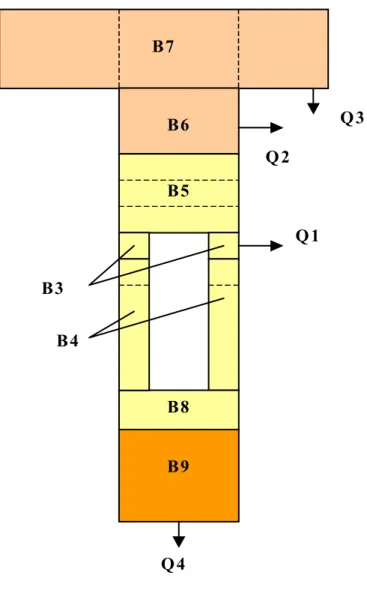
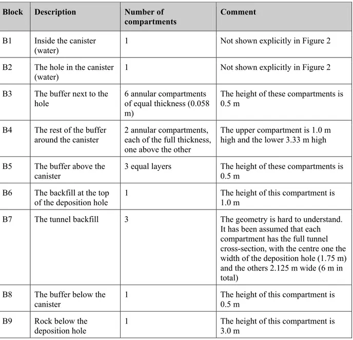
Figure 2 and Table 3 give details of the modelling blocks used in the near field, some of which are broken down into a number of compartments. Table 4 lists the release

pathways from the near field to the geosphere that have been addressed in the model.

B7 B6 B5 B8 B9 B4 B3 Q1 Q 2 Q 3 Q 4

(30)

Table 3: Near-Field Blocks.

Block Description Number of

compartments

Comment

B1 Inside the canister (water)

1 Not shown explicitly in Figure 2 B2 The hole in the canister

(water)

1 Not shown explicitly in Figure 2 B3 The buffer next to the

hole

6 annular compartments of equal thickness (0.058 m)

The height of these compartments is 0.5 m

B4 The rest of the buffer around the canister

2 annular compartments, each of the full thickness, one above the other

The upper compartment is 1.0 m high and the lower 3.33 m high B5 The buffer above the

canister

3 equal layers The height of these compartments is 0.5 m

B6 The backfill at the top of the deposition hole

1 The height of this compartment is 1.0 m

B7 The tunnel backfill 3 The geometry is hard to understand. It has been assumed that each compartment has the full tunnel cross-section, with the centre one the width of the deposition hole (1.75 m) and the others 2.125 m wide (6 m in total)

B8 The buffer below the

canister 1 The height of this compartment is 0.5 m B9 Rock below the

deposition hole

1 The height of this compartment is 3.0 m

Table 4: Near-Field Release Routes.

Route Location

Q1 From the outer B3 compartment Q2 From the B6 block

Q3 From one of the outer B7 compartments Q4 From the rock below the deposition hole

(31)

5.1.1 Transfers between Near-Field Compartments

Diffusional transfers can take place in horizontal or vertical directions, and these were specified by SKB in terms of resistances between compartments. For diffusion in a given direction, the resistance between compartments i and j is given by:

) ( 2 1 j j j i i i ij A D d A D d ₊ = Ω , 5.1

where A is the area perpendicular to the direction of transport, D is the effective diffusion coefficient, and d is the length of the compartment in the direction of radionuclide transport.

The associated transfer rate between compartment i and compartment j is _λij_{given by:}

ij i ij Ω = κ λ 1 , _5.2

where _κi_{is the capacity of compartment i defined by:} i

i i

i _θ _R _V

κ = , 5.3

where _θi_{is the compartment porosity, R}i _{is the retardation coefficient for the} radionuclide in question and _Vi_{is the compartment volume.}

Analytical expressions are used for the transfer resistances from the source term into the buffer. For the canister-hole resistance we have:

Hole Hole A D d = Ω , _5.4

where dHole is the length of the hole.

The resistance for the buffer-hole interface is taken as:

Hole A D 2π 1 = Ω , _5.5

The four release locations have different properties. The fracture zones (Q1 and Q3) have extra resistance because of the small size, while Q2 and Q4 just have a flow resistance.

(32)

where Aq is a lumped parameter with values 0.03, 0.1, 1 and 1 m2.5 y-0.5 for Q1-Q4 respectively. Here q is the near-field Darcy flux (taken to have a value of 0.002 m y-1). This resistance was considered in Neretnieks (1979) is discussed in more detail in Appendix A.

For Q1 and Q3 additional resistances are added according to

D B

=

Ω , _5.7

where B is another lumped parameter with dimensions m-1_{. For Q1 this had a value of}

0.9 m-1 and for Q3 0.333 m-1. The theory behind this representation is given by Neretnieks (1986).

In the geosphere, the flowing fracture was discretised into 5 compartments, consistent with a Peclet number in the region of 10. Six rock matrix compartments were associated with each fracture compartment, with the sizes of the matrix compartments increasing by a factor of 3 from the fracture to the diffusion limit.

It was assumed that the walls of the fracture compartments (to a depth δ) are in equilibrium with flowing water. This introduces an effective fracture retardation coefficient Rf given by a K R d f ) ( 2 1+ δ θ +ρ = , 5.8

where θis the rock porosity (dimensionless), ρ is its density (kg m-3_{), a is the fracture}

half-aperture (m) and Kd is the relevant equilibrium sorption coefficient (m3 kg-1). This is effectively the same as introducing a very thin first rock matrix compartment, and can be important for strongly sorbed radionuclides. A value for δ of 2×10-3_{m was}

employed.

5.2 Deterministic Calculations

As noted in Section 4.2.8 the SR-Can Interim Report presents no deterministic calculations. Selected deterministic AMBER calculations are presented here with the aim of contributing to an understanding of the important issues that derive from the SKB PA calculations.

5.2.1 Calculations based on SR 97 Parameter Values

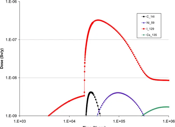
A first set of calculations has been undertaken based on the SR 97 test case parameter values, except that biosphere effective does factors for Beberg were used for well and mire biospheres (Nordlinder et al., 1999).

(33)

Cs-135. There is a very rapid increase in dose soon after the hole in the canister is assumed to increase in size at 20 000 years.

1.E-09 1.E-08 1.E-07 1.E-06

1.E+03 1.E+04 1.E+05 1.E+06

Time (Years) Dose (Sv/y) C_14I Ni_59 I_129 Cs_135

Figure 3: Calculated Doses Using SR 97 Data for a Well Biosphere with 5 Failed Canisters.

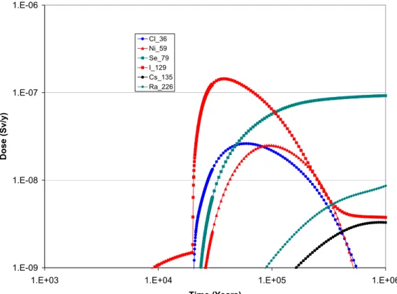
Figure 4 shows corresponding calculations doses for a mire biosphere. The peak dose rate is slightly lower, but a wider range of radionuclides are important: Cl-36, Ni-59, Se-79, I-129, Cs-135 and Ra-226.

(34)

1.E-09 1.E-08 1.E-07 1.E-06

1.E+03 1.E+04 1.E+05 1.E+06

Time (Years) Dose (Sv/y) Cl_36 Ni_59 Se_79 I_129 Cs_135 Ra_226

Figure 4: Calculated Doses Using SR 97 Data for a Mire Biosphere with 5 Failed Canisters.

5.2.2 Calculations based on SR-Can Parameter Values

The AMBER case file used for the calculations presented in Section 5.2.1 was modified to include some key changes in SKB's calculations between SR 97 and the SR-Can Interim Main Report. The aim was to help identify the significance of the changes that have been made.

Table 5 gives details of these changes. Some other parameter values, such as diffusivities, have also changed, but these were considered to be less important and were not implemented in the revised calculations.

The AMBER calculations were undertaken with a fracture half-aperture b of 1×10-4_m.

The implied F value can be calculated (as in Hartley et al., 2004), as T/b, where T is the geosphere transport time in years. This gives F=1×106_{y m}-1_{, towards the bottom end of}

(35)

Table 5: The Main Modifications to the SR 97 Data for the AMBER Deterministic Calculations.

Data SR 97 SR-Can Comments

Biosphere Factors Beberg factors from TR-99-15

Tables A-16 and A-17 in the SR-Can Data Report

Factors can vary by up to about two orders of magnitude for individual radionuclides.

Fuel Dissolution Rate (y-1₎ 1×10

-8_2.75×10-7_{: mid-point of}

data range

The SR-Can range represents an increase by a factor of 50 to 500 over the SR 97 values. Matrix penetration depth (m) 2.0 0.4 Geosphere Travel Time (y) 10 100 SR-Can value is representative of travel times to the terrestrial environment.

Sorption Coefficients

Kd (m3 kg-1)

Bentonite values from Table A-9 in the SR-Can Data Report Rock values from Table A-15 in the SR-Can Data Report

Significant changes from SR 97 values for some radionuclides.

Solubility Data Table A-3 in the SR-Can Data Report

Generally minor

differences between two sets of data.

Near-field Darcy velocity in fracture (m y-1₎

2×10-3 _3×10-5_{: representative}

value from Table 6-3 of SR-Can data report

Used in calculation of near-field transport resistances

'Large' area of hole when sudden increase takes place

0.01 Effectively infinite In SR-Can there is effectively no resistance to radionuclide transport from the canister when the hole increases in size.

(36)

It is understood that SKB did not model explicitly the daughters of Ra-226 (Pb-210 and Po-210) in the near field and geosphere. In addition, Pb-210 is referred to in the

biosphere calculations, but Po-210 is not. However, it is stated in the Interim Report that the results presented for doses from Ra-226 include contributions from its daughters. There is therefore a lack of clarity about the modelling of the bottom end of the U-238 decay chain.

In the calculations presented here, two variants have therefore been considered. The first is where Pb-210 is assumed to be mobile in the near field and geosphere, and the second where it is assumed to have the same transport properties as Ra-226 in these parts of the system. This approach has been taken in order to provide an indication of the

uncertainties that may arise from not modelling the decay chain in full. In both sets of calculations only the biosphere doses from Pb-210 are considered, as no information is available on the biosphere EDF for Po-210.

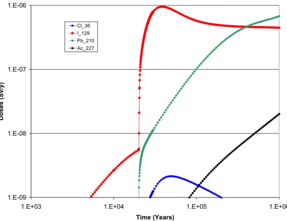
Figure 5 shows the calculated doses for a well biosphere assuming that lead (Pb-210) is mobile in the near field and geosphere. One of the key radionuclides is again I-129, with a peak dose rate of around 1×10-6_{Sv y}-1_{; however, the dose rate from Pb 210 (a}

daughter of Ra-226) is still increasing after a million years. Other important radio-nuclides are Cl-36 and Ac-227 (part of the U-235 decay series). Alternatively, if lead is assumed to have the same transport characteristics as radium in the near field and geosphere, there are no significant contributions from the U-238 decay chain members (so that the curve for Pb 210 does not appear in Figure 5).

1.E-09 1.E-08 1.E-07 1.E-06

1.E+03 1.E+04 1.E+05 1.E+06

Time (Years) D o ses (Sv/ y) Cl_36 I_129 Pb_210 Ac_227

(37)

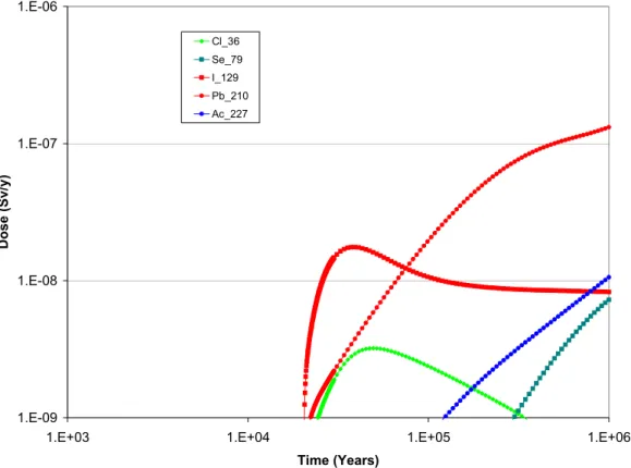
Figure 6 shows the corresponding calculations for a mire biosphere. Peak dose rates are slightly lower than for the well biosphere. As was the case for the well biosphere, if lead is assumed to have the same transport characteristics as radium in the near field and geosphere, there are no significant contributions from the U-238 decay chain members (so that the Pb 210 curve does not appear in Figure 6).

These deterministic calculations are useful in suggesting that the details of the dose calculations have changed as a result of the parameter changes between SR 97 and SR Can, but the overall peak dose calculations are comparable (typically 10-6 to 10-7 Sv y-1 for 5 failed canisters). In addition, the possible importance of detailed modelling of the U-238 decay chain from Ra-226 to Po-210 has been identified.

1.E-09 1.E-08 1.E-07 1.E-06

1.E+03 1.E+04 1.E+05 1.E+06

Time (Years) Dose ( S v/y) Cl_36 Se_79 I_129 Pb_210 Ac_227

Figure 6: Calculated Doses Using SR-Can Data for a Mire Biosphere with 5 Failed Canisters.

5.3 Probabilistic Calculations

Independent calculations have been undertaken for SKB's base case, and for the variant in which all 4500 canisters are assumed to fail after 1×103_{years. For all the AMBER}

runs only 500 samples were used in order to keep the computer run times and the size of the data files produced to a manageable scale. This is adequate to determine the key features of a run, but more samples could be used if required in order to explore

(38)

The geosphere and biosphere data used in SKB’s PA calculations are derived from other code calculations; only statistical summary data are provided in the SR-Can

documentation, and so the precise numbers used are not available.

Probabilistic AMBER calculations were undertaken, with key uncertain parameters being sampled. Table 6 gives details of the sampled parameters.

Table 6: Sampled Parameters in the AMBER Probabilistic Calculations.

Data Parameter Values Comments

Canister failure time 0 to 1×106_years

(triangular, peaking at 1×106_{y) for base case}

1×103_{y (fixed) for case}

with all canisters failing

Allowance is made for 1×103_y

delay time between canister failure and release of radioactivity

Fuel Dissolution Rate (y-1₎ _{Uniform (5×10}-8_{, 5×10}-7₎ _{The SR-Can range represents an}

increase by a factor of 50 to 500 over the SR 97 values.

Time for transport resistance at the canister hole reduces to zero

Uniform (0, 1×105₎

Matrix penetration depth (m) Triangular (0.05, 0.4, 3)

Fracture aperture (m) Uniform (1×10-5_{, 1×10}-3₎ _{Chosen to simulate uncertainty in}

the F factor. This gives a range for the F factor of 1×105_{to 1×10}7_y

m-1_{. Note that fixed values have}

been retained for the lumped parameters in the buffer / fracture interface transport resistance

It should be noted that the mean values for the biosphere EDF's were employed, so there is no contribution to the uncertainty in the overall results for the Quintessa calculations from the biosphere uncertainties.

Table 7 gives details of other sampled parameters in the SR-Can probabilistic calculations that are treated as deterministic in the AMBER calculations.

(39)

Table 7: Sampled Parameters in the SR-Can Calculations retained as Deterministic in the AMBER Calculations.

Data SKB Parameter Values Comments

Solubility Data Table A-3 in the SR-Can Data Report

Buffer Diffusivities Table A-7 in the SR-Can Data Report

Buffer Porosities Table A-7 in the SR-Can Data Report

These are element-dependent, with triangular distribution for anions

Buffer Sorption parameters Table A-9 in the SR-Can Data Report

Backfill Sorption parameters Table A-12 in the SR-Can Data Report

Near-field Darcy velocity q Section 6.5 of data report Statistical information only provided by SKB - no sampling undertaken in the Quintessa calculations

Far-field F factor Section 6.5 of data report Statistical information only. Simulated by variation in fracture aperture in AMBER calculations (see Table 6)

Rock Sorption Coefficients

Kd (m3 kg-1)

Table A-15 in the SR-Can Data Report

Matrix diffusivity values Table A-14 in the SR-Can Data Report

Biosphere Factors Tables A-16 and A-17 in the SR-Can Data Report

Mean values employed - no sampling undertaken in the Quintessa calculations

5.3.1 The Base Case

Figure 7 and Figure 8 show the results of AMBER calculations for the SKB base case where the transport characteristics of Pb-210 in the near field and geosphere are taken to be the same as for Ra-226. The figures show the mean dose and the 95th percentiles for the mean. These follow closely the calculated mean doses in Figures 12-2 and 12-3 of the Interim Report. This demonstrates that the AMBER calculations have satisfactorily

(40)

1.0E-10 1.0E-09 1.0E-08 1.0E-07 1.0E-06

1.0E+04 1.0E+05 1.0E+06

Time (Years) Do ses (Sv/y) Mean Upper 95% Lower 95%

Figure 7: Base Case Calculation for the Well Biosphere.

1.E-10 1.E-09 1.E-08 1.E-07 1.E-06

1.E+04 1.E+05 1.E+06

Time (Years) Do ses (Sv/y) Mean Upper 95% Lower 95%

(41)

If Pb-210 is assumed to be mobile, significantly increased doses are calculated, as illustrated in Figure 9, which can be compared with Figure 8.

1.E-10 1.E-09 1.E-08 1.E-07 1.E-06 1.E+05 1.E+06 Time (Years) Do se (Sv/y) Mean Upper 95% Lower 95%

Figure 9: Base Case Calculation for the Mire Biosphere with Mobile Pb.

The contributions from I-129 and Pb-210 to total dose as a function of time are shown in Figure 10 and Figure 11.

1.E-10 1.E-09 1.E-08 1.E-07 1.E-06 1.E+05 1.E+06

I-129 Dose (Sv/y)

Mean Upper 95% Lower 95%

(42)

1.E-10 1.E-09 1.E-08 1.E-07 1.E-06 1.E+05 1.E+06 Time (Years) Pb-210 Dose (Sv/y) Mean Upper 95% Lower 95%

Figure 11: Base Case Calculation for the Mire Biosphere for mobile Pb-210.

5.3.2 The All Canisters Failed Case

Figure 12 and Figure 13 illustrate the results of calculations for the variant case where all the canisters are assumed to fail after 1000 years. The calculations for the mire biosphere compare well with the SR-Can calculations given in Figure 12-22 of the Interim Report. 1.E-07 1.E-06 1.E-05 1.E-04 1.E-03 1.E-02

1.E+03 1.E+04 1.E+05 1.E+06

Time (Years)

Doses (Sv/y)

(43)

1.E-07 1.E-06 1.E-05 1.E-04 1.E-03 1.E-02

1.E+03 1.E+04 1.E+05 1.E+06

Time (Years) D o se (Sv/ y) Mean Upper 95% Lower 95%

Figure 13: Probabilistic Calculations for the Mire Biosphere with 4500 Failed Canisters.

Figure 14 and Figure 15 give results for the corresponding calculations if Pb-210 is assumed to be mobile in the near field and geosphere. Again, this results in dose rates increasing by about an order of magnitude.

1.0E-07 1.0E-06 1.0E-05 1.0E-04 1.0E-03 1.0E-02

1.0E+03 1.0E+04 1.0E+05 1.0E+06

Dose ( S v/y) Mean Upper 95% Lower 95%

(44)

1.0E-07 1.0E-06 1.0E-05 1.0E-04 1.0E-03 1.0E-02

1.0E+03 1.0E+04 1.0E+05 1.0E+06

Time (Years)

Doses (Sv/y)

Figure 15: Probabilistic Calculations for the Mire Biosphere with 4500 Failed Canisters with Mobile Pb.

Figure 16 gives the percentile plot for the mire biosphere corresponding to Figure 15. This illustrates the wide range of dose rates calculated for the 500 samples. At a million years, the difference between the 5th and 95th percentiles is around 3 orders of

magnitude. 1.0E-07 1.0E-06 1.0E-05 1.0E-04 1.0E-03 1.0E-02

1.0E+03 1.0E+04 1.0E+05 1.0E+06

Time (Years)

Doses (Sv/y)

5% 50% 95%

(45)

Figure 17 and Figure 18 give some scatter plots for this calculation. It can be seen that there appears to be a positive correlation between dose rate from Pb-210 and the fuel dissolution rate, but not with the maximum matrix penetration depth.

1.E-09 1.E-08 1.E-07 1.E-06 1.E-05 1.E-04 1.E-03 1.E-02 1.E-01

1.0E-08 1.0E-07 1.0E-06

Fuel Dissolution Rate (y^-1)

Pb-210 Dose (Sv/y)

Figure 17: Scatter Plot of Dose Rate from Pb-210 at 1×106 Years against Fuel Dissolution Rate. 1.E-09 1.E-08 1.E-07 1.E-06 1.E-05 1.E-04 1.E-03 1.E-02 1.E-01 0 0.5 1 1.5 2 2.5 3 Pb-210 D o se (Sv/y)

(46)

5.4 Summary

The key points that have emerged from the AMBER calculations can be summarised as follows:

1. The lack of any deterministic calculations in the SR-Can Interim Report is unfortunate, as these can provide the basis for an understanding of the most important features of the safety assessment. Without these, it is more difficult to ensure a full understanding of the implications of the probabilistic calculations that have been undertaken.

2. The SR-Can probabilistic calculations use output from hydrogeological

calculations, and only summary data have been presented in the Interim Report. This means that a full reproduction of the SR-can probabilistic calculations was not possible.

3. Probabilistic AMBER calculations with selected use of sampled parameters from SR-Can have nevertheless provided very similar results to those in the Interim Report for both the Base case and the variant where all canisters are assumed to fail simultaneously.

4. There remain uncertainties over how SKB have modelled the U-238 decay chain, and whether this could affect the calculated doses significantly. AMBER calculations that assume the daughters of Ra-226 are mobile (not sorbed) in the near field and geosphere give calculated dose rates that are typically an order of magnitude higher than obtained under the assumption that they have similar transport properties to the parent.

5. As discussed in Appendix A, there remain uncertainties over the details of how SKB have modelled the transport resistance at the buffer-fracture interface. Fixed values for the lumped transport resistance parameters were employed in the AMBER calculations reported here.

(47)

6 Conclusions

The main conclusions that have been drawn can be summarised as follows:

1. The effects of climate evolution on engineered barriers have not been analysed in detail in the Interim Report, and this limits the usefulness of the preliminary calculations that have been undertaken.

2. A key aspect of SKB's approach is the use of an integrated near-field evolution model. The information provided on this model demonstrates its capability efficiently to reproduce calculations from individual process models, but insufficient information is given at the present time to justify statements about interactions between processes. In particular it is assumed that relatively short-term thermal and resaturation processes do not affect the properties of the buffer and its longer-term performance.

3. The underlying methods for considering radionuclide transport are little changed from SR 97, although useful improvements have been made in some areas. The approach taken means that additional calculations are needed to address issues related to the evolution of the system with time. Whether the overall

methodology will enable a comprehensive assessment to be undertaken in practice can only be judged when the full SR-Can assessment is available. 4. The documentation of the models used in PA calculations often relies on

references going back over a period of twenty years updated by model validity documents for each model. The production of a single up-to-date supporting document giving full details of the models used would greatly assist the transparency of the safety case presentation.

5. The consideration of conceptual uncertainties in the supporting Process Report is restricted to the buffer. This restriction greatly limits the usefulness of the Process Report in providing information on the overall methodology. For example, it is not clear whether the approach taken for the buffer will be satisfactory for addressing conceptual model uncertainties in the geosphere. 6. SKB have not presented any deterministic PA calculations. Without these it is

often difficult to understand fully the probabilistic calculations that are presented, although independent AMBER calculations have been able to

reproduce the key features of these calculations. It is suggested that deterministic calculations should be part of SR-Can safety assessment.

7. It has been possible to reproduce the key features of the interim SR-Can probabilistic calculations with AMBER, although there remain uncertainties deriving from the way that SKB have modelled the U-238 decay chain in different parts of the system.