Do Retail Investors Benefit From a High Dividend Yield? : The Dogs of the Dow strategy applied on the Swedish stock market.

MASTER THESIS WITHIN: Business Administration &

Finance

NUMBER OF CREDITS: 30 hp

PROGRAMME OF STUDY: Civilekonom AUTHOR: Daniel Gerson Frisö

TUTOR: Urban Österlund & Tina Wallin JÖNKÖPING 05 2016

Do Retail Investors Benefit

From a High Dividend

Yield?

The Dogs of the Dow strategy applied on the Swedish

stock market.

I

Acknowledgments

First of, I would like to thank my supervisors PhD. Urban Österlund and Doctoral Candidate Tina Wallin along with all the students in our seminar group who have provided me with feedback these past months, that has improved the thesis enormously. I would also like to thank Adina Alic and Johan Ideskog for all the hours we have spent discussing and for all the feedback they have given me, which has led to improvements and an overall better thesis.

Daniel Gerson Frisö Jönköping, May 2016

Abstract

In this thesis, the ten stocks with the highest dividend yield from the OMXS30 have been used to construct a portfolio, a strategy called The Dogs of the Dow. The portfolio was equally weighted and rebalanced every year. The purpose of this thesis is to see how the strategy would perform in terms of return and risk compared to the market. To define the market two indexes were used, OMXSPI and OMXSGI, which excludes and includes dividends respectively. A low dividends portfolio was also used as a benchmark. Though beating the market some individual years and showing a tendency of performing better in an up-going market, the strategy's average annual return of 9.69 percent for the whole period only beat one of the benchmarks. The strategy's risk was fairly similar to the market risk hence, it does not compensate the lower return with lower risk. The Sharpe ratio showed that the Dogs of the Dow portfolio had the best risk adjusted return in only two out of the eleven years. This points towards the conclusion that the strategy would not have performed better, overall, compared to the benchmarks between the years of 2005 and 2015.

II

1

Introduction ... 1

1.1 Background ... 2

1.2 Problem Discussion ... 3

1.3 The Swedish Market ... 4

1.4 Purpose and Research Questions ... 4

1.5 Delimitations ... 5

1.6 Methodology & Disposition ... 5

2

Theoretical Framework ... 7

2.1 Dividend Policy and the Demand for Dividends ... 7

2.2 Dogs of the Dow Studies ... 7

2.3 Dog of the Dow Articles With Methods Used in This Study ... 11

2.4 Log Returns vs. Simple Returns ... 16

3

Method ... 17

3.1 Sub-periods ... 18

3.2 Data ... 19

3.3 Portfolio Construction ... 20

3.4 Evaluation of the DoD strategy ... 21

3.5 Statistical Significance ... 22

4

Results and Analysis ... 23

4.1 The companies ... 23

4.2 Return ... 25

4.3 Abnormal Return and Sub-periods ... 27

4.4 Dividend ... 33

4.5 Risk and Risk Adjusted Return ... 34

5

Discussion ... 38

5.1 The Performance of the DoD Portfolio and the Benchmarks ... 38

5.2 Implications of the Findings ... 40

5.3 Limitations and Method Critic ... 41

6

Conclusion ... 42

III

Appendix ... 46

Appendix 1: Companies included in the low dividend portfolio ... 46

Appendix 2: Portfolio value and return down-going sub period ... 47

Appendix 3: Portfolio value and return up-going sub period ... 48

Appendix 4: Company categories of the DoD portfolio ... 49

IV

Tables

Table 1: Previous Dog of the Dow studies ... 15

Table 2: Dogs of the Dow companies throughout the years ... 24

Table 3: Total yearly return ... 27

Table 4: Yearly Abnormal Returns of the DoD Portfolio (t-statistic) ... 29

Table 5: Bear market 07/2007-12/2008 ... 32

Table 6: Bull market 01/2009-05/2011 ... 32

Table 7: Difference in Dividend ... 34

Table 8: Standard Deviation ... 35

Table 9: Sharpe Ratios ... 35

Figures

Figure 2: Standardized return during the down-going period ... 30

Figure 3: Standardized return during the up-going period ... 31

V

Key Terms

Retail Investor: An individual investor that invests her/his private money.

Benchmark: A pre-determined comparison, in this case the low-dividend portfolio, OMXSGI and OMXSPI.

Dividend: The total amount paid out from a company to its shareholders during a year, including ordinary and extra dividend as well as in the form of new stocks.

Dividend yield: The total amount of dividend paid out per share during one year divided by the current share price.

OMXS30: A weighted index of the 30 biggest companies, with respect to trade volume on the Stockholm stock exchange

OMXSGI: A weighted index for all shares notated on the Stockholm stock exchange including dividend.

OMXSPI: A weighted index for all shares notated on the Stockholm stock exchange excluding dividend.

Sharpe Index/Ratio: A risk adjusted measure of the return developed by William Sharpe (1966).

1

1 Introduction

____________________________________________________________________

In Chapter One, an introduction to the topic is given together with a short background after which the purpose and the research questions are stated and a

delimitation of the topic is given.

___________________________________________________________________

How about getting an amount of money into your account on a yearly basis without you having to do anything. Perhaps this is too good to be true now that interest rates are at a historical low (André Meiton, 18 Jan. 2016), but maybe the dividend paid by a stock could work as a replacement for interest to some extent. Investing in a company’s stock means becoming one of the owners of that company and as an owner you should be able to get a part of the revenue. This is one reason why companies pay out dividend. Investing in stocks that have high dividend yield (i.e. dividend-to-price ratio) could therefore be attractive. For people without expert knowledge about the stock market many things could seem confusing in the beginning. However, understanding that a dividend yield of four percent is higher than two percent should be quite easy even for a stock market novice. Therefore this is perhaps something one can take advantage of when building a stock portfolio.

Trading with stocks has become something that almost everybody has access to and is able to do. It just takes a couple of minutes to set up an account at an internet broker and you are set. After taking another couple of minutes to get to know the brokers website, one can easily sort the companies after their dividend yield. One is by then ready to construct a portfolio consisting of high dividend yield companies. Constructing the portfolio consisting of high dividend yield stocks is not much more complicated than putting money into your savings account, but is it better? There is a consensus among experts that it is beneficial for the individual to have their savings exposed towards the stock market as long as they have a long time horizon for their savings (Lieber, 8 Jan. 2016). This can be done in several ways, for example by buying funds or directly investing in stocks. With the different alternatives come different levels and types of risks. Losing one’s life savings would for almost anybody be devastating, so keeping

2

the risk low, or at least to a level at which you are able to sleep at night, is of course an important part when choosing between investments.

When investing, choosing the stocks of relatively big companies can give the investor a certain level of confidence in that the risk of default is not as big as it is when investing in a small company. Because of that, investing in the highest dividend yielding stocks, which also are some of the biggest companies on the market, is perhaps a preferable way to go. Companies, whose stocks have shown growth over decades, perhaps even centuries together with a yearly payment in cash. To sum up, there is a possibility of, with very little effort, letting your money grow and getting a yearly payment in cash without taking a too big risk. Again this maybe is too good to be true it is, however, worth looking into further.

1.1 Background

Dogs of the Dow, (DoD) is the name of the investment strategy first presented by Johan

Slatter in an article in the Wall Street Journal 1988 (Vähämaa & Rinn, 2011). In short, the original strategy was that investors should buy the ten highest dividend yielding stocks of the Dow Jones Industrial Average (DJIA) the first trading day of the year. The portfolio should be equally weighted and after a year, rebalanced by which stocks are then the highest dividend yielding. There are also other variants of the strategy e.g. one only picks the five highest dividend yielding (Da Silva, 2001). The first step of the DoD strategy is to calculate or retrieve the dividend yield of all the stock on an index containing the biggest companies on the market. Usually the index will contain approximately 30 companies (for example, DJIA, OMXS30, OMXH25 and the Toronto 35 Index). Thereafter you chose the ten stocks with the highest dividend yield and invest an equal amount in them. This is all done in the beginning of the year according to the original strategy, although there are several variants of the starting date. The dividend received during the year is reinvested in the stock and when the year comes to an end, the procedure of picking the top-ten is then repeated.

3

1.2 Problem Discussion

Even though the main idea of the DoD investment strategy is that it is an easy way to beat the index, originally the DJIA, the performance of the strategy fluctuates in different research. With several papers testing the performance of the DoD strategy (e.g. Da Silva, 2001, ap Gwilym, Seaton and Thomas, 2005 and Visscher & Filbeck, 2003) and drawing different conclusions on its performance it is possible that certain market attributes, specific to the market tested, can affect the DoD strategy’s performance. With the possibility of market characteristics affecting its performance one should be hesitant to draw major conclusions from previous studies that were done on other markets than the Swedish. As argued above the simplicity of the strategy is what makes it appealing. It is also possible for retail investors to, in an easy way, construct a DoD portfolio. This motivates the usage of a retail investor’s perspective when researching the strategy’s performance. The chosen perspective of a retail investor broadens the problem in the sense that, having a source confirming or rejecting the performance over the chosen benchmark is crucial for individuals to be able to trust in the investment strategy. This is because, not every retail investor can take the time, or has the knowledge, to perform empirical tests with historical data before deciding whether to build a portfolio or not, independent on whichever strategy the portfolio in question may be based on.

The objective with this thesis is to clarify whether the strategy will work or not on the Swedish market. The existing literature leaves room for further evaluation of the DoD strategy on the Swedish stock market in particular, since it is the US market that is the market most thoroughly tested so far. Together with the fact that the DoD investment strategy seems, according to previous literature (see table 1 for an overview of the current literature) to give different results depending on the market that it is tested upon.

To conclude the problem discussion, since the DoD strategy was developed there have been several attempts to evaluate its performance. With fluctuating results in previous research, another attempt to assess a high dividend yield based portfolio will be done in this thesis. This will contribute to the existing literature by analyzing the effectiveness

4

of the strategy on a different market and adding a piece to the puzzle of whether it is a valuable strategy from an economical view.

1.3 The Swedish Market

Why is it theninteresting to look at the Swedish market when there already exist studies conducted around the world? Rinne and Vähämaa (2011) discuss the reasons why applying the DoD strategy on the Finnish stock market can result in different conclusions than when applied on the US stock market. They say that the small number of companies listed on the Finnish market compared to the US is one of the specific differences. This difference is true as well for the Swedish market compared with the US. Another characteristic of the Swedish stock market that differentiates it from the US stock market is the small number of stocks, with a few companies having a large market capitalization. There are also many firms listed with a small market capitalization (Lidén, 2007).

In previous studies, the argument has been laid out that even if the DoD strategy creates abnormal returns, they are not big enough to cover transaction costs and taxes. The fact behind the argument is that dividend was taxed more heavily than return gained from price changes (see McQueen, Shield & Thorley, 1997 and ap Gwilym, Seaton & Thomas, 2005). In Sweden there are today new forms of saving accounts (investeringssparkonto) that use a standard tax rate based on the current interest rate level and do not take into consideration differences between dividend and price returns. For that reason the taxation will not differ between investing in high dividend paying stocks or low.

1.4 Purpose and Research Questions

The purpose of this thesis is to investigate how the DoD strategy, if applied on the Swedish stock market by a retail investor, will perform against the market, and whether the strategy would have a higher or lower risk than the market. The thesis will investigate the strategy in terms of its return and its risk and compare it to benchmarks

5

that will be used to define the market as well as to an alternative low dividend portfolio. To fulfill the purpose of the thesis the following research questions will be stated:

• Would the DoD strategy, if applied on the Swedish stock market generate a greater return than the benchmarks?

• How does the risk in the DoD portfolio compare to the benchmarks’ risks? 1.5 Delimitations

The thesis is delimited in two ways: First of, the thesis considers only the Swedish market. Other studies have investigated the DoD strategy on several different markets such as the US, Canadian and Finnish. The varying result from previous research is further reason to only include the Swedish market, as well is the perspective of a retail investor, which is applied in this thesis. This contributes also to the easy-to-follow attribute of the strategy. Further, this thesis will closely follow the original DoD strategy, which was based on the DJIA, therefore OMXS30 will be the base from which the DoD portfolio will be constructed. As the DJIA, OMXS30 consists of 30 major companies and is, like the DJIA based on the most traded stocks on the market. (Nasdaq OMX Nordic, 2016)

Secondly, the period that will be investigated will not go back any further than to 2005. The fast evolution of technology has made trading with stocks accessible for the masses. This motivates not going back too far in time. Another reason comes from that if one would go back further in time it would be easy to slip in to the burst of the it-bubble in the beginning of the 21st century. With two crises within the test period the results may become biased. Because of obvious reasons, such as access to data, the test period will be up until and including 2015.

1.6 Methodology & Disposition

In empirical research and within finance in particular, a positivistic view is frequently held. A view that implies that what is perceived as a truth is rooted in what can be observed and proved from an objective standpoint. A reason for such a view can be

6

traced to the fact that the subject of finance is often empirical in itself (Ryan, Scapens & Theobald, 2002). Due to the thesis’ purpose a positivistic methodology is adopted whereby empirical methods will be used to try to fulfill the purpose and answer the above stated research questions.

The rest of the thesis is structured as follows: in Chapter Two the theoretical framework of the thesis is given. In that chapter the theories surrounding the Dogs of the Dow strategy are presented as well as other theoretical concepts that are of interest for this thesis. Articles and literature were gathered by searching databases such as Primo. In this review, onlyarticles on the DoD topic that have been published and peer reviewed are presented. In Chapter Three the method used to fulfil the purpose is presented. The results follow in Chapter Four together with an analysis. A broader discussion and suggestion on further research is given in Chapter Five. To end the thesis, the results are concluded in Chapter Six.

7

2 Theoretical Framework

___________________________________________________________________

In Chapter Two the theoretical framework that surrounds the thesis is given. This will give the reader the results from previous studies and the knowledge needed to

understand the method used and the results of the thesis.

___________________________________________________________________ 2.1 Dividend Policy and the Demand for Dividends

The dividend policies of companies have been discussed in many academic papers during several decades. Modigliani and Miller (1961) suggested that a company’s dividend payout policy does not matter in a perfect market. Hence, it will not affect the value of the company’s shares. The important part here being that it applies under perfect market conditions. Textbooks in corporate finance still refer to the Modigliani and Miller (1961) dividend irrelevance theorem. However, since the early 1960’s the view of how the payout policy influences a company´s value has shifted. Still keeping some of the original assumptions of a perfect market, DeAngelo and DeAngelo (2006) states that the payout policy of a company will affect the company’s value. Either way, one can confirm by looking through the literature that there exist investors with a preference for dividend, both retail and institutional investors (Dong, Robinson & Veld 2005, Graham & Kumar 2006). In theory the possibility of recreating cash dividend by selling stock is often mentioned, Shefrin & Stateman (1984) argues the contrary, meaning that selling stocks should not be seen as a perfect substitute for receiving dividend. They also argue that, in some cases, there exists a willingness to pay a premium on the share price to be able to receive cash dividends. The reason for this, seen as quite odd behavior to some, is to minimize the risk of feeling regret if the sold share will increase in value soon after the investor has sold it.

2.2 Dogs of the Dow Studies

The literature surrounding dividend investing is extensive and there are several papers that are dedicated to the DoD strategy specifically. To get an overview of the existing

8

literature a review of the articles was conducted. Articles were gathered by a thorough search of databases such as Primo with the key words; Dogs of the Dow and dividend

investing. Some articles were found by being referred to in newer articles. The articles

are divided into two sections, first are articles that have applied the DoD strategy but which methods are not explained thoroughly in the article itself. Thereafter, articles, with methods, that are more deeply explained and, that possibly are of use for this thesis are presented. The results from all articles that have applied the DoD strategy are summarized in Table 1 at the end of the section.

As briefly mentioned above, the DoD strategy seems to first appear in the Wall Street

Journal in 1988. In a column written by John Slatter, at that time working as an analyst,

evidence was presented that investing in the ten highest dividend yielding stocks of the DJIA would give a return of 18 percent compared to the market return of 11 percent. The return was the annual average during the sample period of 1972-1987 (Filbeck & Visscher, 1997). The strategy was further made popular when a couple of books were published confirming the, at that time, unquestionable success of the DoD strategy (see O’Higgins & Downes, 1991 and Knowles & Petty, 1992). In the books, the original DoD strategy was applied, just as before, on the DJIA. The periods investigated in both of the books, though they go back a bit further than previously, are similar to the period first tested by Slatter. This could be one obvious reason as to why all of the studies confirm the success of the strategy.

After that the DoD strategy itself was tested, researchers started to look for reasons for its success. In a study conducted by Domian, Louton and Mossman (1998) it was hypothesized that the performance of the DoD strategy can be linked to a ‘winner-loser effect’. In their study, Domian et al. (1998) formed two portfolios, one with the high yield stocks and one with low yield, and for their benchmark, they used the S&P 500 as the market portfolio. Then they tested the performance of the portfolios twelve months before and after the portfolios where set up. The results implied that stocks included in the high dividend portfolio had been underperforming before the portfolio was set up, and therefore had a high dividend yield. Hence, the high return can be traced back to a normalization of the stock price by the market. The opposite was true for the low

9

dividend portfolio. The stock in that portfolio had over performed compared to the market prior to the portfolio construction.

Hirschey (2000) presents several reasons that he argues can explain the excess return found in previous studies. He points towards data mining and errors in the choice of test periods. In addition he states that the strategy’s easy to understand attribute and the way it has been marketed are reasons for its popularity. Hirschey (2000) argues that there does not exist any real evidence proving that the DoD strategy does create excess return compared to the DJIA. Da Silva (2001) conducted a study of the DoD strategy on the Latin American markets of Argentina, Brazil, Chile, Colombia, Mexico, Peru and Venezuela The study looked at 97 percent of the total Latin American and Caribbean stock markets, measured in market capitalization. Da Silva (2001) tested several versions of the DoD strategy, these were; top ten, top five, top one, and the second highest dividend yielding stock on its own. The strategy was also tested with different starting days, this to see if seasonal factors impact the performance. The portfolios were started on the first trading day of January, in accordance with the original strategy. An alternative starting day was set to the first trading day in July due to it being as far away from January as possible. To measure the risk adjusted return of the portfolios the Sharpe index was calculated. The portfolios were compered against a broad index for each of the markets. Da Silva (2001) does deduct both taxes and transaction costs from the return. The returns were calculated from the adjusted price of the stock and were calculated monthly. The risk-free rate used for the Sharpe index was a three month deposited rate from the individual country. He found that, despite evidence suggesting that the strategy may be successful in all countries except for Brazil the findings did not have statistical significance due to the short test period.

Up until the mid 2000s most of the academic literature on DoD often had its focus on the US market. However, starting in 2005, several papers applied the DoD investment strategy upon different markets around the world (e.g. Alles F Fin & Tze Sheng, 2008, Tai-Leung Chong & Keung Luk, 2010 and Rinne & Vähämaa, 2011). In Alles F Fin & Tze Sheng (2008) the DoD was evaluated on the Australian stock market between the years of 2000 and 2006. They set up a portfolio containing the ten highest dividend yielding stock as of December 31. The stocks were picked from the S&P/ASX 50

10

Index. The returns were continuously compounded and calculated annually. They found that the strategy did produce abnormal returns compared, in this case, with the expected returns calculated via the Capital Asset Pricing Model using data from the ASX All Ordinaries index. In their results they also argued that the abnormal return would hold for transaction costs. Another study that tried to explain the reasons behind the, now somewhat questioned, investment strategy was carried out by Wang, Larsen, Aninina, Akhbari & Nicolas (2011). They suggested that it is herding and the individual’s irrational behavior that are the reasons for why the DoD strategy works. They tested the investment strategy on the Chinese stock market where their findings, they argue, are in line with the behavioral finance theory of that any inefficiencies in the market can be traced back to the above mentioned human behavior.

As a contrast to the above articles that were all written from an academic point of view, Clemens (2011) investigates dividend investing from a practitioner’s view. He shows that a portfolio containing high dividend yield will have a higher return. He tests, between 1992-2012, both the strategy on the US market as well as the world market using world indexes. Clemens (2011) argues that the companies paying out dividend will face lower agency costs that are usually associated with stock buy backs, acquisitions of other companies or mergers, and that it could be a reason for the better performance of those companies’ stocks.

ap Gwilym, et al. (2005) sorted out the 350 biggest companies on the UK stock market measured by market capitalization and created several benchmarks out of them. These are the 100 biggest, the next 250 and then all of the 350 companies. They also used the FT 30 index, which they argue is the one that most closely resembles the DJIA. Portfolios consisting of the top-five and top-ten dividend yielding stock were created from all benchmarks. The portfolios were set up like the original DoD strategy on the first trading day of the year, they were equally weighted and held for one year. An equally weighted portfolio consisting of all the stocks in the FT 30 index was also set up. Like in the study by McQueen et al. (1997) the risk was adjusted by investing at the risk free rate and the transaction costs were assumed to be one percent. Their findings suggested that any return higher than the market disappeared when the strategy was adjusted for risk and transaction costs.

11

Chong & Luk (2011) tested two versions of the DoD strategy on the Hong Kong market. Both were created at the end of the year and were equally weighted. One consisted of the top-ten dividend yielding stocks listed on the Hong Kong Stock Exchange and the second consisted of the top five stocks of the Hang Seng Index, the sum of 1 000 000 USD was invested in each of the strategies. The returns were calculated by simple return (see eq. 3). They found that the results differed between the two indexes. The strategy applied on the Hong Kong Stock Exchange gave a negative return of almost 1.3 percent. Whilst the strategy applied on the Hang Seng Index provided a positive return of over 8 percent. However, for reasons left out in their paper, the different strategies were only applied on one of the benchmarks. They did not apply the top-ten strategy upon the Hang Seng index and vice versa.

These articles mentioned above are some of those written within the topic of dividend investing and concerning the DoD investment strategy. Articles that use methods of greater importance for this thesis will be presented below. Where the different methods used by researchers, both when it comes to constructing the portfolio and when evaluating the portfolio, will be explained more in depth to give the reader a good basis for Chapter Three.

2.3 Dog of the Dow Articles With Methods Used in This Study

McQueen et. al (1997) formed portfolios that consisted of both the top-ten highest dividend yielding stocks as well as all the 30 stocks of the DJIA. The portfolios were created in the beginning of the year and held intact for the remaining year, and both of them were equally weighted. The dividend was reinvested in the stock that paid it at the end of the month. McQueen et al. (1997) used the last quarterly dividends payment, which they annualized, and the price of the stock at the end of the year to calculate the dividend yields. First, they compared the return of the two portfolios with each other. Thereby they found that the top-ten portfolio outperformed the portfolio consisting of all the stocks with three percentage points, which they found to be statistical significant. However, to get a more fair comparison, hence, risk adjusting the returns, McQueen et al. (1997) invested a portion of the total wealth of the top ten-portfolio in Treasury bills

12

so that the standard deviation of the two portfolios was the same. That meant that 13 percent of the total top-ten portfolio value was invested in Treasury bills, shrinking the difference of the returns from three percent to 1.5 percent. Drawing from this result, the conclusion is that most of the abnormal return can be associated to the higher risk in the top-ten portfolio. To fully answer their main question, further deductions were made for transaction costs. Since the top-ten portfolio on average changed almost three firms each year, to compare to only 0.35 firms per year for the comparison portfolio, they argued that with transaction costs of one percent, only 0.95 percentage points in difference between the two portfolios remain. Due to big differences in taxes depending on individual circumstances McQueen et al. (1997) were not able to make any deduction for tax, however they still stated that the strategy would probably not work.

Filbeck and Visscher (1997) applied the DoD strategy on the British market. They calculated the dividend yields of all of the 100 stocks on the Financial Times-Stock Exchange 100 Index on the first of March instead of on the first trading day of the year because the index was created in February 1984. They took the ten stocks with the highest yield and created a portfolio by investing 1 000 GBP in each of the stocks. The returns were calculated by, simply adding the price change with eventual dividend and then dividing the sum with the price in the beginning of the month. After a year they started all over again by investing a new 1 000 GBP in that years ten stocks with the highest dividend yield. The risk free rate was calculated every month and consisted of the twelfth root from the sum of one plus the 90-day Treasury bill return. They compered the top-ten portfolio with the Financial Times-Stock Exchange 100 Index, from which the portfolio was created, by calculating the difference between the top-ten and the market return. They also performed a paired difference test to get the t-statistic. For, as they say, comparison reasons, Filbeck and Visscher (1997) calculate the Sharpe index as well as the Treynor index. They calculated the Sharpe index by dividing the difference of the return (either the top ten portfolio or the market) and the risk-free rate with the standard deviation of that difference and then multiplying the quotient with the root out of 12. They argued that the Sharpe index is the most appropriate measurement in the case when the investor is exposed to company specific risk, i.e. when the portfolio is not fully diversified. The opposite is then true for the Treynor index, hence, it should be the measurement of choice when the portfolio is well diversified and the

13

risk is systematic. The Treynor measure is the difference of the return (either the top ten portfolio or the market) and the risk-free rate divided by the respective beta. Their results indicate that the DoD investment strategy does not perform better than the market. During their test period of 1984-1994 the DoD portfolio beat the market in only four individual years. They lift the fact that they compared the portfolio against an index of a 100 stock as a reason for why it did not perform better when studies comparing against the DJIA, which only has 30 stocks, had shown that the strategy does work.

A portfolio consisting of the top-ten, highest dividend yielding stocks, was created from the Toronto 35 Index by Visscher and Filbeck (2003). In their study they hypothesized that the top-ten portfolio would beat the Toronto 35 Index as well as the broader TSE 300 index. They used the 31 of July as their starting and rebalancing date, one reason was because the Toronto 35 Index was created in March the same year as their sample period started and they wanted to give the index a few months to settle. The second reason was to avoid effects from possible tax trading on the last trading day, when they created their portfolio. The procedure followed closely the procedure of Filbeck and Visscher (1997). The returns were calculated monthly by adding the price change with the dividend and dividing the sum by the price of the stock in the beginning of the month. The portfolio value was determined by investing 10 000 CAD in each of the stocks and then multiplying it with the stock’s return and summarizing the values. After a year, they repeated the procedure by again investing 10 000 CAD in each stock included in the top-ten portfolio. Just like in previous studies, Visscher and Filbeck (2003) calculated both the Sharpe ratio and the Treynor index via the difference between the top-ten portfolio return and the index return. They also used the difference between the return i.e. the abnormal return, to calculate the t-statistic by a paired difference test.

𝑡 =_!!

! ∙ 𝑛 − 1 (eq. 1)

Where, 𝑑 is the difference between the portfolio and market return, 𝑆_! is the standard deviation of the difference between the returns and 𝑛-1 is degrees of freedom.

14

Visscher and Filbeck (2003) made assumptions about both the tax rate and the transactions costs, whereby they exaggerated the tax disadvantage by setting the marginal tax for the top-ten portfolio to 40 percent and 20 percent for the index return. The transaction costs they assumed to be 1 percent of the total portfolio value. In this case the found the strategy producing higher return than the index, even after being risk adjusted. Both the Sharpe ratio and the Treynor ratio were found to be higher for the DoD portfolio than for the Toronto 35 Index.

Rinne and Vähämaa (2011) applied a different statistical technique to evaluate the DoD strategy that they argued would help avoid problems such as small sample bias. They tested the investment strategy on the Finnish market, which they believe has certain characteristics that are not found on other markets yet tested e.g. relatively few companies listed and one company making up a large proportion of the whole market. They followed the original DoD strategy, where on the last trading day the dividend yield is calculated by dividing the dividend paid out during the year with the current share price and an equally weighted portfolio was created. The portfolio was held for a year after which they rebalanced it to whichever ten stocks had the highest dividend yield. The stocks were picked from the OMXH25 index, which is similar to the OMXS30 index. To evaluate the strategy Rinne and Vähämaa (2011) calculated abnormal returns, defined as:

𝐷𝑜𝐷_!" = 𝐷𝑜𝐷_! − 𝐵𝑒𝑛𝑐ℎ𝑚𝑎𝑟𝑘_! (eq. 2)

Where, DoDAR is the DoD portfolio’s abnormal return, DoDR is the return of the DoD

portfolio and BenchmarkR is the benchmark’s return.

In order to prevent small sample bias, they use a bootstrapping approach whereby they took 10 000 random samples with the mean and median of the abnormal return to calculate non-parametric confidence intervals. Rinne and Vähämaa (2011) showed that the DoD strategy on the Finnish market during the period 1988-2008 would give an abnormal return of, on average, 4.5 percent yearly. Their findings point towards that the DoD strategy can be successful on the Finnish stock market but they also mention that the result may lack economical significance. Meaning that the transaction costs and taxes might be too high for the abnormal return to survive compared to the index return.

15

Table 1: Pervious Dogs of the Dow studies

* Annual average

1_{Reported average monthly data annualized}

2_{The reported excess return against the 350 largest stocks}

3

Average of the reported yearly returns

Work Period Market DoD

portfolio return* Benchmark index return* Difference Slatter (1997) 1972-1988 USA 18.4 % 10.8 % 7.6 % O’Higgins & Downes (1991) 1973-1991 USA 16.6 % 10.4 % 6.2 %

Knowles & Petty (1992) 1957-1990 USA 14.2 % 10.4 % 3.8 % McQueen et. Al (1997) 1946-1995 USA 16.8 % 13.7 % 3.1 % Filbeck & Visscher (1997) 1985-1994 UK 9.5 % 11.6 % -2.1 % Hirschey (2000) 1961-1998 USA 14.2 % 12.4 % 1.8 % Da Silva (2001)1 1994-1999 Argentina Brazil Chile Colombia Mexico Peru Venezuela 8.3 % 17.3 % 15.9 % -2.8 % 10.6 % 9.8 % 15.9 % 5.9 % 35.6 % 4.3 % -4.7 % 8.0 % 9.0 % 11.1 % 2.4 % -18.3 % 11.6 % 1.9 % 2.6 % 0.8 % 4.8 % Visscher & Filbeck (2003) 1988-1997 Canada 15.1 % 9.0 % 6.1 % ap Gwilym, et al. (2005) 1980-2001 UK N/A N/A 2.7 %2

Alles F Fin & Tze Sheng (2008)3 2000-2006 Australia 18.5 % 8,9 % 9.6 % Tai-Leung Chong & Keung

Luk, (2011) 1993-2007 Hong Kong (two indexes) -1.28 % 8.61 % N/A N/A Rinne and Vähämaa (2011) 1988-2008 Finland 15.5 % 11.0 % 4.5 %

16

2.4 Log Returns vs. Simple Returns

In almost every financial article the term return is used, but it is not always specified how it is calculated. There are two main ways that returns can be calculated, either simple returns or log returns, which are also known as continuously compounded returns. Which to choose can be of importance for understanding the research and being able to draw conclusions from the empiric findings in the future. (Dorfleitner, 2003) Simple return and log return are defined respectively as:

𝑅_!"#$%& = !"#$%!

!"#$%!!!− 1 (eq. 3)

Where, 𝑉𝑎𝑙𝑢𝑒 is the total portfolio value in dollar terms at time t.

𝑅_!"# = ln 𝑉𝑎𝑙𝑢𝑒_!!! − ln (𝑉𝑎𝑙𝑢𝑒_!) (eq. 4)

Where, 𝑉𝑎𝑙𝑢𝑒 is the total portfolio value in dollar terms at time t.

The advantages of using log returns are its additive properties. If a multi-period is to be examined, it is possible to simply add together several single-period log returns. However, the log returns, unlike the simple returns, will not be the same as the true value change stated in terms of money (Hudson & Gregoriou, 2015). Dorfleitner (2003) argues that when a portfolio is to be considered as the interest of the research, the simple return calculation is the most appropriate, and that is therefore the method of choice in this thesis.

17

3 Method

___________________________________________________________________

In Chapter Three, an extensive explanation of how the research was carried out is given, as well as a description of the method used to answer the research

questions.

___________________________________________________________________

By sorting the OMXS30 by which stocks have the highest dividend yield, a portfolio was set up of those that have the ten highest yields. Monthly data from 2005 up until and including 2015 was used. By applying the investment strategy to this period, the data contained an up-going trend, a financial crisis as well as a recovery of the stock market, in other words both, so called, bull and bear markets. Therefore, the evaluation of the strategy is done both over the entire period and broken in to sub-periods. Hence, it will be possible to analyze the performance of the investment strategy during a specific period, such as an economical downturn.

What determines whether the portfolio has been successful, or not, is dependent on both which method is used to calculate the return and to against what the return is compared. Having a suitable benchmark to compare the portfolio against is crucial. Three specific benchmarks were used in this thesis to assess the investment strategy, where two are indexes, which will represent the market. Indexes can be categorized into two broad categories. The first one is when the index measures exclusively the price changes in the market. In that case, the dividend is not taken into account, i.e. the dividend from companies is deducted when the index value is calculated. The second category is when the dividend is taken into account. This gives a measure of how the total return of the index moves as it adds the dividend paid out together with the price changes of the stocks. (Nasdaq OMX Nordic, 2016).

First, the broad index OMXSPI was used to compare the strategy’s performance against the market. This index includes all the stocks listed on Nasdaq OMX (i.e. Stockholm stock exchange) and therefore gives a good picture of how the Swedish stock market has developed. However, OMXSPI does not contain any dividends, it is a

price-18

development-only index, because of that, OMXSGI is used as a complement. It is also a broad index containing all the stocks listed on the Stockholm stock exchange, but with the difference that it will show how the market, including dividend has developed. This creates a more fair comparison against the DoD portfolio since OMXSGI does not exclude any economical gain, such as dividend. A third benchmark, which is used, is a portfolio consisting of the ten stocks with lowest dividend yield on the OMXS30. This creates the option of analyzing the question if the dividend yield is a reason in itself for a more or less successful portfolio.

The benchmarks:

• Benchmark 1: Low dividend portfolio (based on OMXS30) • Benchmark 2: OMXSPI (excluding dividend)

• Benchmark 3 OMXSGI (including dividend)

A common measure that is used when it comes to comparing portfolio’s performance is the Sharpe ratio (Sharpe, 1966), which takes into account the risk, or more specifically the standard deviation, of the portfolio. The Sharpe ratio provides a number, which will be comparable among the different portfolios. The advantage of the Sharpe ratio is that it considers company specific risk and it is therefore suitable when the portfolio is not well diversified (Visscher & Filbeck, 2003). With the different risks accounted for, it provides a better measure of the performance of the portfolios as well as being comparable to other investment strategies.

3.1 Sub-periods

The period that was studied was between 2005 and 2015. Besides the whole period several sub-periods were studied as well. These consist of both individual years and of periods with down-going and up-going market. The down-going period was between September 2007 and December 2008. In this period, the broad market index, OMXSP, does not exceed previous levels at any time.

19

The up-going period starts with the recovery from the financial crisis in January 2009 and ends in May 2011. Within this period, the index does not fall more than two consecutive months. The period ends due to a four-month decline of the OMXSPI. The periods of the down-going and up-going trends were chosen by studying the graph over the entire period of 2005-2015. After approximated periods were chosen from the graph, the OMXSPI index price was studied in detail to find trends and to set more precise start and end dates. The sub-periods: Down-going market (bear market), September 2007 to December 2008 and up-going market (bull market), January 2009 to May 2011.

3.2 Data

Data containing the closing prices and the dividend paid out was the main data used in this thesis, the closing prices were taken monthly. This data is gathered from Thomson DataStream as well as from the individual companies’ annual reports when necessary. The data that was used is historical data both for the dividends paid and the closing price. The data collected on the dividend is the total dividend paid out during the year. This will therefore include, apart from the ordinary dividends, extra dividends as well as dividends in the form of stocks. All these different types of dividends are considered in the calculated dividend yield of each company since it is in reality what an individual investor would gain economically. For the purpose of giving an as fair picture as possible, the modified closing price was used to calculate the returns. The modified closing price subtracts any dividend and stock splits. Because of that, it shows the return of the stock without it being affected by dividends of any sort, this will also have the advantage that there will be no risk of letting the dividend have “twice“ the impact compared to the benchmarks. If a company were to be sold and delisted during a year in which they are included in one of the portfolios, the money received from the sell will be kept as cash until the next rebalancing of the portfolio. Nordnet and Nasdaq Nordic proved to be valuable sources, both when it came to answering questions concerning data gathering as well as providing the data in itself.

20

3.3 Portfolio Construction

A portfolio consisting of the companies that currently have the highest dividend yield is set up on the first trading day of the year. It is thereafter held for one year after which it will be rebalanced to, once again be an equally weighted portfolio containing the ten highest dividend-yielding stocks. This procedure was repeated for the entire test period of 2005 to 2015. To be included in the DoD portfolio, the stock should have a top-ten dividend yield, which is defined as the total dividend payment during the preceding year divided by the current price of the stock. The same procedure goes for the portfolio that consists of the ten lowest dividend yielding stocks, the low dividend portfolio, of course with the difference that to be included in that portfolio, the stock most have one of the ten lowest dividend yields. To be able to consider the dividend in the return calculations the fictive sum of 10 000 SEK was used to buy shares in each of the companies respectively. Previous studies have used a similar amount and it will also have the advantage that a fair amount of shares will be able to be bought, combined with the fact that the total amount invested will not be too big from a retail investor’s perspective. This is done on the first trading day of the first year of the test period. As the dividend is paid out it was reinvested in the same stock at the closing price used for the month in which it was received. Contrary to the method used in Filbeck and Visscher (1997) and Visscher and Filbeck (2003), a new 10 000 SEK will not be used to invest in the next year's portfolio. Instead the amount held at the end of the year will be used. This will give a more realistic setting of how the portfolio value changes without affecting the return reported. At the first trading day of the year, the total value of the portfolio from the previous year will be divided equally between the ten stocks that will be included in that year’s portfolio. This procedure is then repeated for every year. By multiplying the closing prices with the number of shares of each stock the total value of the portfolio is retrieved.

Portfolio value = 𝑆ℎ𝑎𝑟𝑒𝑠_! × 𝐶𝑙𝑜𝑠𝑖𝑛𝑔 𝑃𝑟𝑖𝑐𝑒_! (eq. 5)

Where Sharesi is the total number of shares owned of a specific company and Closing

Pricei is the closing price of that stock. The return of the portfolio stock is calculated by

21

calculated monthly, as monthly data is gathered. Simple returns were calculated since it is the most suitable in the specific case of this thesis, because of that the research focuses on portfolio performance. For the index benchmark the simple return was calculated based on its closing price and also in this case, monthly.

3.4 Evaluation of the DoD strategy

To evaluate the DoD portfolio in accordance with previous conducted studies the abnormal return was calculated. This led as well to getting results that were comparable between studies. The abnormal return was also the result that was the base for the statistical testing. The return of the DoD portfolio was subtracted by the returns of the benchmarks, each individually, to generate any abnormal returns, defined as in equation 2:

𝐷𝑜𝐷_!" = 𝐷𝑜𝐷_! − 𝐵𝑒𝑛𝑐ℎ𝑚𝑎𝑟𝑘_!(eq. 2)

Where, DoDAR is the DoD portfolio’s abnormal return, DoDR is the return of the DoD

portfolio and BenchmarkR is the benchmark’s return.

The Sharpe ratio was calculated for the DoD portfolio as well as for all the benchmark portfolios. This will enable a comparison of the performance of the DoD strategy with adjustment for risk. The Sharpe ratio is defined as:

𝑆ℎ𝑎𝑟𝑝𝑒 𝑟𝑎𝑡𝑖𝑜 = !!"#$%"&'"!!!

!".!"#.!"#$%&#'(# (eq. 6)

Where, 𝑅_!"#$%"&'" is the portfolio return, 𝑅_!is the risk-free rate and 𝑆𝑡. 𝐷𝑒𝑣._!"#$%&#'(# is the standard deviation of the portfolio return. The risk-free rate was held constant for one year and is the rate of the ten-year Swedish government bond taken on the first trading day of the specific year.

22

3.5 Statistical Significance

Comparing the different portfolios and the index’s returns can in itself give an indication on the performance. A problem arises when the differences between the portfolios are small. To ensure reliable results and conclusions there needs to be statistical significance behind the findings. A t-test can help determine if the difference between, in this case two returns, is significantly different. This is a simple statistical test which will give a deeper insight in to the findings, in particular how the return findings of the DoD investment strategy stands against its benchmark returns. (Anderson, Sweeney, Williams, Freeman & Shoesmith, 2014)

To secure the robustness of the results, previous studies have calculated the t-statistic and performed a t-test on the abnormal returns of the DoD portfolio. This was done as well in this thesis. Following earlier studies, a paired difference test was calculated with the t-statistic defined as in equation 1.

If statistical significance does exist, conclusions can be drawn from the difference in performance between the DoD portfolio and the benchmark. The null hypothesis tested is that the abnormal return is equal to zero, with the alternative hypothesis of that the abnormal return is not equal to zero, defined as:

𝐻_!: 𝐷𝑜𝐷_!" = 0 𝐻!: 𝐷𝑜𝐷!" ≠ 0

The evaluation of the portfolio was done in several ways, as has been discussed above. First there is the abnormal return of the DoD portfolio. This gave an indication of how much more, or less, return the investments strategy has generated compared to each of the benchmarks individually. Secondly, the Sharpe ratio showed the performance of the portfolio adjusted for risk. The Sharpe ratio was compared between the DoD portfolio, the low dividend portfolio and the indexes. The comparison gave a picture of the portfolios’ and indexes’ performances adjusted for the individual level of risk in each of them. Lastly, the abnormal return of the DoD portfolio was checked for statistical significance by a t-statistic.

23

4 Results and Analysis

___________________________________________________________________

In Chapter Four the results from the research will be presented and analyzed. The companies included in the portfolio will be presented first, followed by the returns

and last the risk of the DoD portfolio.

___________________________________________________________________ 4.1 The companies

The companies that appeared in the DoD portfolio are presented in table 2 below, as well as which year(s) they were included. In total, there were 32 companies that at some point were included in the DoD portfolio during the period investigated. On average, there were 3.3 new companies in the portfolio every year, the turnover of companies each year is similar to the results of McQueen et al. (1997). TeliaSonera is the only company that is included in the DoD portfolio every year.

Of the 32 companies eight are in the category industrial goods and services, banks and basic resources are the two categories that follow with four companies each. In 2015, there are 4 banks in the portfolio, this is also the most companies within one category included during the test period. During the period, there are a total of 13 categories represented at some point in the DoD portfolio (see appendices 5.4 and 5.5 for a full specification of the categories).

The industry categories of which the companies within the DoD portfolio belong to show no strong patterns during the test period. There is though a tendency of banks having high dividend yields from about the second half of the period and staying in the portfolio from that point on. Swedbank enters the DoD portfolio in 2011 followed by both Nordea and SEB in 2012. This could perhaps depend on normalization effects of both the stock price and dividend level after the financial crisis. Both Nordea and Swedbank are in the portfolio before and during the crisis. Due to the drop in the stock prices during this period it is the dividend in itself that lowers the dividend yield the period after the crisis and up until when they re-enter the portfolio. This suggests that the crisis forced the banks to hold on to their money and not pay out dividends to the stockholders.

24

Table 2: Dogs of the Dow companies throughout the years

2005 2006 2007 2008 2009 2010 2011 2012 2013 2014 2015 Alfa Laval X AstraZeneca X X X X X X X Atlas Copco A X Atlas Copco B X X Boliden X X X X Fabege X Electrolux X Eniro X X Ericsson B X X X X HM X X Holmen B X X Investor B X Lundin Petroleum X MTG B X X X Nokia X X X X X X Nordea X X X X X X X Sandvik X X X SCA B X X X X Scania X X SEB A X X X X Securitas X X X X X SHB X Skanska X X X X X X X X X X SKF B X X SSAB A X Stora Enso R X Swedbank4 _{X X X X X X X} Swedish Match X Tele2 X X X X X X X X X TeliaSonera X X X X X X X X X X X Wihlborgs X Volvo B X X X 4

Swedbank was traded under the name Föreningssparbanken up until 2006 but for convenience Swedbank is the only name that is used in this thesis.

25

Because of the spread of companies among 13 industry categories, the investment strategy gives the investor the benefit of diversity among company categories, which contributes to lowering the risk. One cannot say, even with the variety of companies included, that the portfolio is fully diversified due to that only ten stocks are included, however. The level of diversification varied also between the years. This has the implication that the return can, in some years, be heavily dependent on a certain category. In 2015, for example, 40 percent of the portfolio consisted of banks. Having that much weight of one sector in the portfolio exposes the investor to high risk. This is contrary to the often used argument that the DoD strategy as a safer strategy.

4.2 Return

Figure 1, below, shows how the portfolios and indexes develop during the entire test period. In the figure the amount earned is reinvested every year, no value that was created is taken out from the portfolios. i.e. the portfolios will receive the effect of compound interest, or as in this case, return. The figure shows clearly that the DoD portfolio does not outperform any index, nor the low dividend portfolio. The figure also indicates that the strong performance of the low dividend portfolio kicks off right after the financial crisis of 2008.

26

Figure 1: Standardized return during the whole period

In table 3, the returns for the individual years are presented as well as the average yearly return. The table confirms the picture given by figure 1. In addition, the DoD portfolio has the highest single year return during the whole period, this was in 2009 when the return of the portfolio was over 91 percent. The worst return of the DoD portfolio was not surprisingly in 2008 when the portfolio had a return of -36.22 percent. However, this return was not worse than either of the indexes that year, which both had a negative return of over 40 percent. All the yearly returns are between the span of 91.30 percent as highest and -45.83 as lowest. Comparing the annual averages, the DoD portfolio has the third highest out of the four. Still, its average return is higher than the OMXSPI index. In some years it is beneficial to invest in the DoD portfolio, but it will not generate a greater return then the benchmarks over a longer period.

The result of the average yearly return being higher than the broad OMXSPI is inline with most of the previous research. Only Filbeck & Visscher (1997) and Da Silva (2001) (in Brazil) find negative abnormal return for the DoD portfolio against the benchmarks used. However, here it is also clear that the choosing of the benchmark

0 100 200 300 400 500 600 700 01-2005 05-2005 09-2005 01-2006 05-2006 09-2006 01-2006 05-2007 09-2007 01-2008 05-2008 09-2008 01-2009 05-2009 09-2009 01-2010 05-2010 09-2010 01-2011 05-2011 09-2011 01-2012 05-2012 09-2012 01-2013 05-2013 09-2013 01-2014 05-2014 09-2014 01-2015 05-2015 09-2015 DoD Low Dividend Por8olio OMXSPI OMXSGI

27

plays an important part in the results, since the DoD portfolio has a negative average yearly return when compared against the OMXSGI.

Table 3: Total yearly return

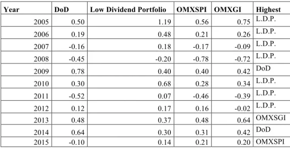
Year DoD Low Dividend portfolio OMXSPI OMXSGI Winner

2005 24.95% 41.09 % 26.32 % 30.59 % L.D.P. 2006 8.47 % 18.44 % 22.16 % 24.15 % OMXSGI 2007 -22.18 % 26.27 % -5.40 % -2.10 % L.D.P. 2008 -36.22 % -21.37 % -45.83 % -43.43 % L.D.P. 2009 91.30 % 61.21 % 39.90 % 45.19 % DoD 2010 15.77 % 36.19 % 17.23 % 20.50 % L.D.P. 2011 -17.77 % 5.98 % -19.98 % -17.18 % L.D.P. 2012 6.15 % 8.66 % 8.61 % 12.95 % OMXSGI 2013 24.86 % 12.39 % 17.83 % 22.23 % DoD 2014 16.63 % 8.30 % 10.63 % 14.40 % DoD 2015 -5.4 1% 8.62 % 10.89 % 10.04 % OMXSPI Average 9.69 % 18.71 % 7.49 % 10.67 % L.D.P.

The three years that the DoD portfolio had the individual year highest return came in 2009 and then again in 2013 and 2014. The first year, 2009, was right after the financial crisis. It was a year when the stock market was in an up-going trend. This pattern is true for the pair of winner years of 2013 and 2014 as well, though it had not been a crisis the year before, the market was still in an up-going trend.

In the DoD portfolios of 2008, 2009 and 2010 there are many industrial goods and services and some basic material companies included. This could be an explanation of the better performance during the years after the 2008 crisis. These types of companies can be especially sensitive to the current market condition, taking a big beating during the crisis. That leads in turn to the possibility of a greater recovery the years after. Both the big beating and then the recovery could possibly be overreactions of the market, as well as that the recovery could be the effect of normalization of the stock price.

4.3 Abnormal Return and Sub-periods

The abnormal returns of the DoD portfolio compared to the benchmarks are presented in table 4 together with the associated t-statistic (calculated as presented in eq. 1). The

28

standard deviation is shown as well, because it is included in the t–statistic calculation. In total, the DoD portfolio had 12 positive abnormal yearly returns, three against the low dividend portfolio, five against OMXSPI and four against OMXSGI. Again, it is 2009 that is the most successful year for the portfolio with an abnormal return of over 51 percent as highest, against OMXSPI. The worst abnormal return was in 2007 against the low dividend portfolio, that year the abnormal return was -48.46 percent. Overall the DoD has five years with positive abnormal return as best, those were against the OMXSPI index. The greatest loss is against the low dividend portfolio where the DoD portfolio only creates a positive abnormal return in three out of eleven years. In total, 25 of the 33 observed abnormal returns are statistically significant different from zero on at least the 90 % confidence level.

Most of the independent years abnormal return against the benchmarks were found to be statistically significant on at least the 90 % confidence level. Due to n-1 degrees of freedom equaled ten, the significance became highly dependent on the difference between the returns. The abnormal return against the low dividend portfolio had only one year of not being statistically different from zero, a lot due to the high difference in return between the portfolios. Against the indexes, there were four and three years of statistical insignificance for the abnormal return against OMXSPI and OMXSGI respectively. Even though it can seem as much when faced with only eleven observations, the results point towards that the DoD portfolio follows the index closely for several individual years. This is also inline with what can be seen from figure 1. As mentioned in section 1.3, the Swedish market has a few companies with a large market capitalization. This means that they weigh heavily when the weighted indexes are calculated, and if these companies also are included in the DoD portfolio it could be a reason for why the portfolio and index follow each other closely. This is an effect that is hard to avoid due to the DoD properties, since the portfolio is based on some of the biggest companies on the market. Having that somewhat troublesome property leads to that the DoD strategy will have it tougher to beat the market. This gives also an indication of the importance of the benchmark, since the outcome can differ if a non-weighted index would be chosen instead.

29

DoD-Low Div. DoD-OMXSPI DoD-OMXSGI

2005 -16.14 %*** (-2.32253109) -1.37 % (-0.219654487) -5.64 %** (-0.950657301) 2006 -9.8 %*** (-1.435279871) -13.69 %*** (-2.190251551) -15.68 %*** (-2.643338955) 2007 -48.46 %*** (-6.971721278) -16.78 %*** (-2.685143005) -20.08 %*** (-3.384955934) 2008 -14.84 %*** (-2.135640509) 9.62 %*** (1.53868014) 7.21 %** (1.215976159) 2009 30.10 %*** (4.330194519) 51.40 %*** (8.223124403) 46.11 %*** (7.771695578) 2010 -20.42 %*** (-2.93730183) -1.46 % (-0.233125602) -4.73 %* (-0.796887421) 2011 -23.76 %*** (-3.417790278) 2.21 % (0.353862312) -0.59 % (-0.099350383) 2012 -2.51 % (-0.361019296) -2.46 % (-0.393647095) -6.80 %** (-1.145814043) 2013 12.46 %*** (1.792943211) 7.03 %** (1.124045442) 2.63 % (0.443130855) 2014 8.33 %** (1.198119352) 6.00 %** (0.959879223) 2.23 % (0.375556463) 2015 -14.03 %*** (-2.018323591) -16.30 %*** (-2.607592101) -15.45 %*** (-2.603569111) St.Dev. 20.85 % 18.75 % 17.80 % *𝐻! rejected on the 90 % confidence level **𝐻! rejected on the 95 % confidence level ***𝐻! rejected on the 99 % confidence level

Da Silva (2001) has a similar testing period of ten years and found that his results lacked statistical significance. His return results indicated however that the DoD portfolio could give positive returns against the market. The results of this thesis point towards a bigger uncertainty as to whether the DoD strategy beats the market or not. Therefore, not having abnormal returns statistically different from zero does not change the findings since the findings are that the DoD portfolio does follow the index to some extent.

30

Moving on to the sub-periods of the down-going (bear market) and up-going (bull market), figures 2 and 3 show the standardized development during those periods. During the bear market the DoD follows the indexes development closely, ending up just above them as 2008 ends. The low dividend portfolio is the benchmark that loses the least during this period and the only one that beats the DoD portfolio. Looking at figure 3, the results are similar. The DoD portfolio did perform better than both indexes during the period, but in the end a bit worse than the low dividend portfolio. However, the DoD portfolio has a higher return than the low dividend portfolio in 14 out of 29 months.

Figure 2: Standardized return during the down-going period

0 20 40 60 80 100 120 140

31

Figure 3: Standardized return during the up-going period

In the bear market sub-period between the fall of 2007 and 2008, the DoD portfolio came out just a bit over the indexes in terms of value development (see figure 2). The results are also confirmed by the average monthly return. The low dividend portfolio does out perform both the indexes and the DoD portfolio, just as in the case of the whole period. In the bear market, the DoD portfolio does perform better than the indexes, comparing their Sharpe ratios. Its risk is also lower than the low dividend portfolio, though its return is worse, which is the main reason for the difference in the Sharpe ratio.

During a crisis, investors often look for safer companies to invest in, they seek for so-called value shares, mature companies that usually have a good dividend payment. The fact that the low dividend portfolio as created from companies on the OMXS30 could be a possible explanation for it not performing worse than it does. Since the way it is created means that it still includes some of the most traded and largest companies on the Swedish stock market, which might still be seen as value stocks by investors. The results of the DoD portfolio beating the market during the bear market are in accordance with the results from Rinne and Vähämaa (2011) who found that the DoD strategy worked particular well when the market was in a down-going trend. However, they did not have a low dividend portfolio as a benchmark.

0,00 50,00 100,00 150,00 200,00 250,00

32

Table 5: Bear market 07/2007-12/2008

DoD Portfolio

Low Dividend

Portfolio OMXSPI OMXGI

Average Monthly Return -3.33 % 0.12 % -4.26 % -4.06 %

St.Dev. 0.07 0.10 0.06 0.06

Sharpe Ratio -0.51 -0.02 -0.78 -0.74

In the bull market the difference between the DoD portfolio return and the benchmarks’ returns are smaller than in the bear market. The risk of the DoD portfolio is similar to the indexes’ risk, and its Sharpe ratio comes out a bit over OMXPI and the low dividend portfolio but worse than OMXSGI as shown in table 6. The result of the DoD portfolio having a higher Sharpe ratio than the low dividend portfolio is a bit surprising when one compares the results from the whole period. Studying the risk and return during the bull market it can be seen that it is the lower risk of the DoD portfolio that drives the higher Sharpe ratio, since the return is lower. These results are somewhat opposite to those of that the DoD performs better in a down-going market. An explanation in this case can again be the fact that the portfolio contains those company categories that can make a big recovery after a crisis such as industrial goods and services and some basic material. One should though be careful to draw too big conclusions due to that only one up-going period is investigated.

Table 6: Bull market 01/2009-05/2011

DoD Portfolio

Low Dividend

Portfolio OMXSPI OMXGI

Average Monthly Return 2.79 % 3.26 % 2.57 % 2.90 %

St.Dev. 0.06 0.08 0.06 0.06