Lossless Message Compression
Bachelor Thesis in Computer Science
Stefan Karlsson
skn07007@student.mdh.se ehn05007@student.mdh.se
Erik Hansson
School of Innovation, Design and Engineering
Mälardalens Högskola
Västerås, Sweden
2013
ABSTRACT
In this thesis we investigated whether using compression when sending inter-process communication (IPC) messages can be beneficial or not. A literature study on lossless com-pression resulted in a compilation of algorithms and tech-niques. Using this compilation, the algorithms LZO, LZFX, LZW, LZMA, bzip2 and LZ4 were selected to be integrated into LINX as an extra layer to support lossless message compression. The testing involved sending messages with real telecom data between two nodes on a dedicated net-work, with different network configurations and message sizes. To calculate the effective throughput for each algo-rithm, the round-trip time was measured. We concluded that the fastest algorithms, i.e. LZ4, LZO and LZFX, were most efficient in our tests.
Keywords
Compression, Message compression, Lossless compression, LINX, IPC, LZO, LZFX, LZW, LZMA, bzip2, LZ4, Effective throughput, Goodput
SAMMANFATTNING
I detta examensarbete har vi unders¨okt huruvida komprimer-ing av meddelanden f¨or interprocesskommunikation (IPC) kan vara f¨ordelaktigt. En litteraturstudie om f¨orlustfri kom-primering resulterade i en sammanst¨allning av algoritmer och tekniker. Fr˚an den h¨ar sammanst¨allningen uts˚ags al-goritmerna LZO, LZFX, LZW, LZMA, bzip2 och LZ4 f¨or integrering i LINX som ett extra lager f¨or att st¨odja kom-primering av meddelanden. Algoritmerna testades genom att skicka meddelanden inneh˚allande riktig telekom-data mel-lan tv˚a noder p˚a ett dedikerat n¨atverk. Detta gjordes med olika n¨atverksinst¨allningar samt storlekar p˚a meddelandena. Den effektiva n¨atverksgenomstr¨omningen r¨aknades ut f¨or varje algoritm genom att m¨ata omloppstiden. Resultatet visade att de snabbaste algoritmerna, allts˚a LZ4, LZO och LZFX, var effektivast i v˚ara tester.
Special thanks to:
Ericsson Supervisor: Marcus J¨agemar Ericsson Manager: Magnus Schlyter MDH Examiner: Mats Bj¨orkman IRIL Lab Manager: Daniel Flemstr¨om
Table of Contents
1 Introduction 3
1.1 Contribution . . . 3
1.2 Structure . . . 3
2 Method for literature study 3 3 Related work 4 4 Problem formulation 5 5 Compression overview 6 5.1 Classifications . . . 6 5.2 Compression factors . . . 6 5.3 Lossless techniques . . . 6 5.3.1 Null suppression . . . 6 5.3.2 Run-length encoding . . . 6 5.3.3 Diatomic encoding . . . 7 5.3.4 Pattern substitution . . . 7 5.3.5 Statistical encoding . . . 7 5.3.6 Arithmetic encoding . . . 7
5.3.7 Context mixing and prediction . . . 7
5.3.8 Burrows-Wheeler transform . . . 8 5.3.9 Relative encoding . . . 8 5.4 Suitable algorithms . . . 8 5.4.1 LZ77 . . . 8 5.4.2 LZ78 . . . 8 5.4.3 LZSS . . . 8 5.4.4 LZW . . . 9 5.4.5 LZMA . . . 9 5.4.6 LZO . . . 9 5.4.7 LZFX . . . 9 5.4.8 LZC . . . 9 5.4.9 LZ4 . . . 9 5.4.10 QuickLZ . . . 9 5.4.11 Gipfeli . . . 9 5.4.12 bzip2 . . . 9 5.4.13 PPM . . . 9 5.4.14 PAQ . . . 9 5.4.15 DEFLATE . . . 10
6 Literature study conclusions 10 6.1 Motivation . . . 10
6.2 Choice of algorithm and comparison . . . 10
7 Method 11 7.1 Test cases . . . 11
7.2 Data working set . . . 12
7.3 Formulas for effective throughput . . . 12
8 Implementation 12 8.1 Test environment . . . 12 8.2 Compression algorithms . . . 13 8.2.1 LZO . . . 13 8.2.2 LZFX . . . 13 8.2.3 LZW . . . 13 8.2.4 LZMA . . . 13 8.2.5 bzip2 . . . 13 8.2.6 LZ4 . . . 14 9 Results 14 10 Conclusion 14 11 Discussion 16 12 MDH thesis conclusion 16 13 Future work 17
1.
INTRODUCTION
The purpose of compression is to decrease the size of the data by representing it in a form that require less space. This will in turn decrease the time to transmit the data over a network or increase the available disk space [1]. Data compression has been used for a long time. One early example was in the ancient Greece where text was written without spaces and punctuation to save space, since paper was expensive [2]. Another example is Morse code, which was invented in 1838. To reduce the time and space required to transmit text, the most used letters in English have the shortest representations in Morse code [3]. For example, the letters ‘e’ and ‘t’ are represented by a single dot and dash, respectively. Using abbreviations, such as CPU for Central Processing Unit, is also a form of data compression [2]. As mainframe computers were beginning to be used, new coding techniques were developed, such as Shannon-Fano coding [4, 5] in 1949 and Huffman coding [6] in 1952. Later, more complex compression algorithms that did not only use coding were developed, for example the dictionary based Lempel-Ziv algorithms in 1977 [7] and 1978 [8]. These have later been used to create many other algorithms.
Compressing data requires resources, such as CPU time and memory. The increasing usage of multi-core CPUs in today’s communication systems increases the computation capac-ity quicker compared to the available communication band-width. One solution to increase the communication capacity is to compress the messages before transmitting them over the network, which in theory should increase the effective bandwidth depending on the type of data sent.
Ericsson’s purpose with this work was to increase the avail-able communication capacity in existing systems by simple means, without upgrading the network hardware or modi-fying the code of existing applications. This was done by analysing existing compression algorithms, followed by in-tegrating a few suitable algorithms into the communication layer of a framework provided by Ericsson. The communica-tion layer in existing systems can then be replaced to support compression. Finally, testing was performed to determine the most promising algorithms. Since this implementation was used in Ericsson’s infrastructure, the message data was very specific. There was no need to test a variety of different data sets, i.e. the compression was done on data gathered from a real system.
1.1
Contribution
We have tested how the performance of LINX IPC mes-sages of sizes between 500 and 1400 bytes sent over a simple network are affected by implementing an extra layer of com-pression into LINX, and at which network bandwidths and message sizes it is beneficial to use such an implementation. We also provide a general idea of what types of compression algorithms to use when sending small sized messages over a network and what affects their performance.
1.2
Structure
This report starts with an introduction to compression, the purpose of this work, the contribution and the structure of this report in Section 1. In Section 2 the method used to find sources for the literature study is described, followed by re-lated work in Section 3 where we summarize papers that are related to our work. Section 4 describes the task and what
we did and did not do in this thesis. Section 5 contains an overview of how compression works, including compression classification, some of the techniques used in compression and suitable compression algorithms for our work. In Sec-tion 6 we drew a conclusion from the literature study and motivated which algorithms we chose to use in our work, as well as describing their properties. Section 7 describes the method for the work. This section includes where we integrated the chosen algorithms, how the message trans-fer was conducted, the test cases used, a description of the data used in the tests and how we calculated the effective throughput. In Section 8 we describe how we integrated the compression algorithms and where we found the source code for them. Here we also describe the hardware used and the network topology, i.e. the test environment. Section 9 con-tains the results of the tests and in Section 10 we draw a conclusion from the results. In Section 11 we discuss the re-sults, conclusion and other related topics that emerged from our work. Section 12 contains the thesis conclusions that are of interest for MDH. Finally Section 13 contains future work.
2.
METHOD FOR LITERATURE STUDY
To get an idea of the current state of research within the field of data compression, we performed a literature study. Infor-mation on how to conduct the literature study was found in Thesis Projects on page 59 [9]. We searched in databases using appropriate keywords, such as compression, lossless compression, data compression and text compression. When searching the ACM Digital Library1 with the com-pression keyword, we found the documents PPMexe: Pro-gram Compression [10], Energy-aware lossless data compres-sion [11], Modeling for text comprescompres-sion [12], LZW-Based Code Compression for VLIW Embedded Systems [13], Data compression [1], Compression Tools Compared [14], A Tech-nique for High Ratio LZW Compression [15] and JPEG2000: The New Still Picture Compression Standard [16].
By searching the references in these documents for other sources, we also found the relevant documents A block-sorting lossless data compression algorithm [17], Data Compression Using Adaptive Coding and Partial String Matching [18], A method for construction of minimum redundancy codes [6], Implementing the PPM data compression scheme [19], Net-work conscious text compression system (NCTCSys) [20], A universal algorithm for data compression [7], Compres-sion of Individual Sequences via Variable-Rate Coding [8], Longest match string searching for Ziv-Lempel compression [21], A corpus for the evaluation of lossless compression al-gorithms [22], PPM Performance with BWT Complexity: A New Method for Lossless Data Compression [23], The math-ematical theory of communication [4], PPM: one step to practicality [24], A Technique for High-Performance Data Compression [25], The Transmission of Information [5], Data Compression via Textual Substitution [26] and The Data Compression Book [27].
Searching the ACM Digital Library with the keywords loss-less compression yielded the additional documents Energy and Performance Evaluation of Lossless File Data Compres-sion on Server Systems [28] and An Analysis of the Burrows-Wheeler Transform [29].
We also searched the IEEE Xplore database2using the
key-words compression, lossless compression, data compression, high speed compression algorithm and text compression and found the documents Lossless Compression Using Efficient Encoding of Bitmasks [30] and Improving Code Density Us-ing Compression Techniques [31], LIPT: a lossless text trans-form to improve compression [32], Unbounded Length Con-texts for PPM [33] and Scaling Down Off-the-Shelf Data Compression: Backwards-Compatible Fine-Grain Mixing [34]. Searching the references in these we found the documents Adaptive end-to-end compression for variable-bandwidth com-munication [35], Adaptive online data compression [36], Fine-Grain Adaptive Compression in Dynamically Variable Net-works [37], Efficient end to end data exchange using config-urable compression [38], Gipfeli - High Speed Compression Algorithm [39] and The hitchhiker’s guide to choosing the compression algorithm for your smart meter data [40]. To find more information about specific algorithms we found in the other documents, we searched Google Scholar3 using
the keywords LZMA, LZSS, LZW, LZX, PPM, DEFLATE, BZIP2, LZ4, LZO, PAQ. This way, we found the papers Hardware Implementation of LZMA Data Compression Al-gorithm [41], The relative efficiency of data compression by LZW and LZSS [42] and Lossless Compression Based on the Sequence Memoizer [43]. Looking at the references in these papers we also found the paper A Comparative Study Of Text Compression Algorithms [44].
We also searched the IEEE Global History Network4 using
the keyword compression to find the page History of Lossless Data Compression Algorithms [45].
While searching Google with the key words effective through-put compression and data transmission compression to find more information on how to calculate effective throughput we stumbled upon a few papers addressing the effect of com-pression in network applications and protocols. The pa-pers found were Improving I/O Forwarding Throughput with Data Compression [46], Robust Data Compression of Net-work Packets [47] and A Comparison of Compressed and Uncompressed Transmission Modes [48].
Finally, to find some more recent benchmarks, we also searched Google using the keywords compression benchmarks to find the page Compression Benchmarks [49] and LZ4 - Extremely Fast Compression algorithm [50].
3.
RELATED WORK
In 1949, C. Shannon and R. Fano invented Shannon-Fano coding [4, 5]. Using this algorithm on a given block of data, codes are assigned to symbols in a way that is inversely proportional to the frequency at which the symbols appear. Two years later, D. Huffman developed a very similar but more efficient coding algorithm called Huffman coding [6]. This technique is often used in combination with other mod-ern algorithms, for example with the Burrows-Wheeler trans-form in bzip2 [51] and with LZ77 or LZSS in the DEFLATE algorithm [52].
In 1977, A. Lempel and J. Ziv developed a new compression algorithm called LZ77 which uses a dictionary to compress
2http://ieeexplore.ieee.org/ 3
http://scholar.google.com/
4http://www.ieeeghn.org/
data [7]. The dictionary is dynamic and generated using a sliding window over the input data. A year later, they developed the LZ78 algorithm, which generates and uses a static dictionary [8]. Many algorithms have been developed based on the LZ77 and LZ78 algorithms, such as DEFLATE [52], the Lempel-Ziv-Markov chain algorithm (LZMA) [53] and the Lempel-Ziv-Welch algorithm (LZW) [25].
One category of algorithms used in data compression that is not based on the LZ77 and LZ78 algorithms is Prediction by Partial Matching (PPM). PPM algorithms have been de-veloped since the mid-1980s by for example Cleary and Wit-ten [18], but have become more popular as the amount of RAM in computers has increased. The PPM algorithms uses the previous symbols in the data stream to predict which the next symbol is. One version called PPMd, developed by D. Shkarin in 2002 [24], aimed to have complexity comparable to the LZ77 and LZ78 algorithms. He showed that the al-gorithm could offer compression ratio comparable to LZ77 and bzip2 but with lower memory requirements and faster rate of compression, or offer better compression ratio than LZ77 and bzip2 but with higher memory requirements and compression time, depending on the settings used.
The Burrows-Wheeler transform (BWT), invented by M. Burrows and D. Wheeler in 1994, does not compress data itself but it makes the data more suited for compression with other algorithms [17]. Used with simple and fast algorithms, such as a move-to-front coder, they were able to show that the algorithm had compression ratio comparable with sta-tistical modellers, but at a rate of compression comparable to Lempel-Ziv algorithms.
In Adaptive end-to-end compression for variable-bandwidth communication [35] by Knutsson and Bj¨orkman from 1999, messages were compressed using an adaptive algorithm which changed the compression level depending on the length of the network queue. They showed that the effective band-width could be increased on networks with 1-3 Mbit/s through-put by compressing the data using a comthrough-puter with a 133 MHz CPU.
In Robust Data Compression of Network Packets [47], S. Dorward and S. Quinlan experimented with different com-pression algorithms to improve the performance of packet networks. The experiments were conducted on 125 and 1600 byte packet sizes on a network with 10 kbit/s, 100 kbit/s, 1 Mbit/s and 10 Mbit/s link speed. They concluded that speed is important when compressing network packets, es-pecially if the bandwidth is large when compared to the available computational capacity.
In 2001 N. Motgi and A. Mukherjee proposed a Network conscious text compression system (NCTCSys) [20] which compressed text based data and could be integrated on ap-plication level into different text based network transfer pro-tocols like HTTP, FTP and SMTP. The compression appli-cations tested were bzip2 and gzip together with LIPT (A lossless text transform to improve compression [32]). With this method they where able to reduce the data transmission time by 60-85%.
On the Distributed Computing Systems conference in 2005, C. Pu and L. Singaravelu presented Fine-Grain Adaptive Compression in Dynamically Variable Networks [37] where they applied adaptive compression on data packets using
a fine-grain mixing strategy which compressed and sent as much data as possible and used any remaining bandwidth to send uncompressed data packets. The compression algo-rithms they tried were gzip, bzip2 and LZO which all have different properties regarding rate of compression and com-pression ratio. Their experiments were conducted on a net-work with up to 1 Gbit/s bandwidth and concluded that improvement gained when using the different compression algorithms was reduced as the physical bandwidth increased to the point where it was worse than non-compressed trans-mission. The maximum bandwidth where compression was beneficial was different for each of the algorithms.
In Energy-aware lossless data compression [11] a comparison of several lossless compression algorithms was made by K. Barr and K. Asanovi´c, where not only compression ratio and rate of compression was measured but also memory usage. This study concludes that there are more factors to consider than only the compression ratio, i.e. a fast algorithm with high compression ratio probably uses a lot more memory than its counterparts. This is something that needs to be considered for implementation on the target architecture. Y. Wiseman wrote The relative efficiency of data compres-sion by LZW and LZSS [42] in 2007 where he compared the compression algorithms LZW and LZSS which are based on LZ77 and LZ78, respectively. The study shows that de-pending on how many bits are used for the pointer, and the number of bits for the length component in LZSS, the re-sults will vary. With too many bits, each pointer will take up too much space, and with too few bits the part of the file which can be pointed to will be too small. The efficiency on different file formats is also compared, and it is concluded that LZSS generally yields a better compression ratio, but for some specific types of files, where the number of point-ers generated by LZW and LZSS are almost equal, LZW performs better since its pointers are smaller than those of LZSS.
In the paper Improving I/O Forwarding Throughput with Data Compression [46] B. Welton, D. Kimpe, J. Cope et al. investigated if the effective bandwidth could be increased by using data compression. They created a set of compression services within the I/O Forwarding Scalability Layer and tested a variety of data sets on high-performance computing clusters. LZO, bzip2 and zlib were used when conducting their experiments. For certain scientific data they observed significant bandwidth improvements, which shows that the benefit of compressing the data prior to transfer is highly dependent on the data being transferred. Their results sug-gest avoiding computationally expensive algorithms due to the time consumption.
In 2011 A Comparative Study Of Text Compression Algo-rithms by S. Shanmugasundaram and R. Lourdusamy was published in the International Journal of Wisdom Based Computing [44]. They presented an overview of different statistical compression algorithms as well as benchmarks comparing the algorithms. The benchmarks were focused on algorithms based on LZ77 and LZ78 but also included some other statistical compression techniques. The proper-ties that were compared in the benchmarks were compres-sion ratio and rate of comprescompres-sion.
In The hitchhiker’s guide to choosing the compression al-gorithm for your smart meter data [40], M. Ringwelski, C. Renner, A. Reinhardt et al. performed tests on compres-sion algorithms to be implemented in Smart Meters5. They
tested compression ratio, rate of compression and memory consumption for different algorithms. Besides the test re-sults, which are relevant to us, they also suggest that the processing time of the algorithms are of high importance if the system runs on battery.
In November 2012 M. Ghosh posted the results of a pression benchmark [49] done with a self-made parallel com-pression program called Pcompress [54] which contains C implementations of LZFX, LZMA, LzmaMt6, LZ4, libbsc,
zlib and bzip2. He also showed that some of the algorithms used can still be optimized, for example he optimized LZMA by using SSE instructions which improved the rate of com-pression. The results are fairly new, which makes them very relevant to our work when deciding which algorithms to in-tegrate.
R. Lenhardt and J. Alakuijala wrote Gipfeli - High Speed Compression Algorithm for the 2012 Data Compression Con-ference where they created their own compression algorithm based on LZ77 called Gipfeli [39]. Gipfeli is a high-speed compression algorithm designed to increase the I/O through-put by reducing the amount of data transferred. Gipfeli is written in C++ and the compression ratio is said to be similar to that of zlib but with three times faster rate of compression.
4.
PROBLEM FORMULATION
The task was to take advantage of compression by integrat-ing it into the supplied communication framework used by the Ericsson Connectivity Packet Platform (CPP). The im-plementation should be done in user-mode, to make it easier to maintain the code if the kernel is upgraded. This would however come at the cost of restricted access to resources that are used in kernel-space. We did a literature study to investigate existing compression algorithms. Based on the study, a few promising algorithms were selected for in-tegration and testing to analyse the effect of compression in the existing environment. The communication was done with LINX Inter-Process Communication (IPC) [55] with the compression as an extra layer which hopefully would increase the communication capacity, i.e. each LINX IPC message was compressed and decompressed.
The tests were performed with varying message sizes on dif-ferent network bandwidths, as well as network topologies, to see if the performance of the algorithms changed. The tests were done without any other traffic present, which meant that the tests had full utilization of the bandwidth. We did not test the effect of compression when communi-cating between processes internally in the CPU. Neither did we develop our own compression algorithm due to time con-straints and we did not use adaptive compression methods. The benchmark did not include an analysis of memory usage for the algorithms, instead we left this for future work.
5
System that sends wireless sensor signals to a target device
5.
COMPRESSION OVERVIEW
This section contains a general introduction to compression and its terms.
5.1
Classifications
The two most distinct classifications of compression algo-rithms are lossy and lossless. Lossy compression reduces the data size by discarding information that requires large amounts of storage but is not necessary for presentation. For example by removing sound frequencies not normally perceived by human hearing in an audio file, as in the MP3 audio format. Lossy compression has proven to be effec-tive when applied to media formats such as video and au-dio [27]. However, when using lossy compression it is im-possible to restore the original file due to removal of essen-tial data. Because of this, lossy compression is not optimal for text-based data containing important information [45]. Lossless data compression can be achieved by various tech-niques that reduces the size without permanently remov-ing any data. Compared to lossy compression, the original data can be restored without losing any information. Loss-less data compression can be found everywhere in comput-ing. Some examples are to save disk space, transmitting data over a network, communication over a secure shell etc. Lossless compression is widely used in embedded systems to improve the communication bandwidth and memory re-quirements [30].
Some examples of compression used in different media for-mats can be seen in Table 1.
Compression type Image Audio Video
Noncompressed RAW WAV CinemaDNG
Lossy JPEG MP3 MPEG
Lossless PNG FLAC H.264
Table 1: Compression used in typical media formats
5.2
Compression factors
Compressing data requires execution time and memory to decrease the size of the data. The compression factors used to describe this are rate of compression, compression ratio and memory usage.
The rate of compression, also known as compression speed, is the time it takes to compress and decompress data. The time it will take for an algorithm to compress and decompress the data is highly dependent on how the algorithm works. Compression ratio is how much a set of data can be com-pressed with a specific algorithm, i.e. how many times smaller in size the compressed data is compared to the noncom-pressed data. The definition of compression ratio is:
R = Size before compression
Size after compression (1)
This definition is sometimes referred to as compression fac-tor in some of the papers used in the literature study. We chose to use this definition instead due to the cognitive per-ception of the human mind [56], where larger is better. Memory usage is how much memory a specific algorithm uses while compressing and decompressing. Like rate of com-pression, the memory usage is highly dependant on how the
algorithm works. For example if it needs additional data structures to decompress the data.
5.3
Lossless techniques
Since we were required to use lossless compression, this sec-tion summarizes some of the existing techniques used when performing lossless data compression. Different variants of the techniques discussed in this section has spawned over the years. Because of this, techniques with similar names can be found, but in the end they work in the same way. For example scientific notation works as Run-length encoding, where 1 000 000 is represented as 1e6 or 1 × 10⁶ in scientific notation and as 1Sc06 in Run-length encoding (here Sc is
the special character, corresponding to ∅ in our examples below).
5.3.1 Null suppression
Null or blank suppression is one of the earliest compression techniques used and is described in [1,57]. The way the tech-nique works is by suppressing null, i.e. blank, characters to reduce the number of symbols needed to represent the data. Instead of storing or transmitting all of the blanks ( ) in a data stream, the blanks are represented by a special symbol followed by a number representing the number of repeated blanks. This would reduce the number of symbols needed to represent the data. Since it needs two symbols to encode the repeated blanks, at least three blanks needs to be re-peated to use this technique, else no compression would be achieved. An example can be seen in Table 2 where the first
With invisible blanks With visible blanks
Date Name Date Name 27-11-1931 Ziv 27-11-1931 Ziv
Table 2: Null suppression example
column is what a person would see and the second column is the actual data needed to form this representation. If we would transfer the information as it is we also need to trans-fer all the blanks. The first two blanks before “Date” cannot be compressed but the other blanks can. If we were to trans-fer the information line by line and use null suppression we would instead send the following data stream:
1. Date∅C11Name
2. 27-11-1931∅C10Ziv
Where the symbol ∅ is the special compression indicator character, Ciis an 8-bit integer encoded as a character and
i is the decimal value of the integer in our example. This means that the maximum number of repeating blanks that can be encoded this way is 256, since this is the maximum value of an 8-bit integer.
By encoding the example in Table 2 and using Equation (1) the compression ratio is
R = 43 27≈ 1.59 The total size was reduced by 37.2%.
5.3.2 Run-length encoding
Like null suppression, Run-length encoding tries to suppress repeated characters as described in [1, 25, 44, 45, 48, 57]. The
difference is that Run-length encoding can be used on all types of characters, not only blanks. Run-length encoding also works similar to null suppression when indicating that a compression of characters has been performed. It uses a special character that indicates that compression follows (in our case we use ∅), next is the character itself and last the number of repeats. To achieve any compression, the number of repeated characters needs to be at least four. In the
exam-Original string Compressed string
CAAAAAAAAAAT C∅A10T
Table 3: Run-length Encoding example
ple in Table 3 we reduced the number of characters from 12 to 5, saving 58% space with a compression ratio of 2.4 when using Equation (1) on the preceding page. If Run-length en-coding would be used on a repetition of blanks it would yield an extra character (the character indicating which charac-ter was repeated) when compared to Null suppression. The use of a mixture of several techniques is suggested due to this [57].
5.3.3 Diatomic encoding
Diatomic encoding is a technique to represent a pair of char-acters as one special character, thus saving 50% space or a compression ratio of 2. This technique is described in [57]. The limitation is that each pair needs a unique special char-acter. The number of special characters that can be used are however limited, since each character consists of a fixed number of bits. To get the most out of this technique one first needs to analyse the data that is going to be compressed and gather the most common pairs of characters, then use the available special characters and assign them to each of the most common pairs.
5.3.4 Pattern substitution
This technique is more or less a sophisticated extension of Diatomic encoding [57]. Patterns that are known to repeat themselves throughout a data stream are used to create a pattern table that contains a list of arguments and a set of function values. The patterns that are put into the table could for example be reserved words in a programming lan-guage (if, for, void, int, printf etc.) or the most common words in an English text (and, the, that, are etc.). Instead of storing or transmitting the full string, a character indicating that a pattern substitution has occurred followed by a value is stored or transmitted in place of the string. When de-coding, the pattern substitute character and the subsequent value is looked up in the table and replaced with the string it represents. The string could contain the keyword itself plus the preceding and succeeding spaces (if any exists), which would yield a higher compression ratio due to the increased length of the string.
5.3.5 Statistical encoding
Statistical encoding is a technique used to determine the probability of encountering a symbol or a string in a specific data stream and use this probability when encoding the data to minimize the average code length L, which is defined as:
L =
n
X
i=1
LiPi (2)
Where n is the number of symbols, Li is the code length
for symbol i and Pi is the probability for symbol i.
In-cluded in this category are widely known compression meth-ods such as Huffman coding, Shannon-Fano encoding and Lempel-Ziv string encoding. These techniques are described in [6–8, 44, 45, 48, 57].
Huffman coding is a technique which reduces the average code length of symbols in an alphabet such as a human lan-guage alphabet or the data-coded alphabet ASCII. Huffman coding has a prefix property which uniquely encodes sym-bols to prevent false interpretations when deciphering the encoded symbols, such that an encoded symbol cannot be a combination of other encoded symbols. The binary tree that is used to store the encoded symbols is built bottom up, compared to the Shannon-Fano tree which is built top down [6, 44, 48, 57]. When the probability of each symbol appearing in the data stream has been determined, they are sorted in order of probability. The two symbols with the low-est probability are then grouped together to form a branch in the binary tree. The branch node is then assigned the combined probability value of the pair. This is iterated with the two nodes with the lowest probability until all nodes are connected and form the final binary tree. After the tree has been completed each edge is either assigned the value one or zero depending on if it is the right or left edge. It does not matter if the left edge is assigned one or zero as long as it is consistent for all nodes. The code for each symbol is then assigned by tracing the route, starting from the root of the tree to the leaf node representing the symbol.
Shannon-Fano encoding works in the same way as Huff-man coding except that the tree is built top down. When the probability of each symbol has been determined and sorted, the symbols are split in two subsets which each form a child node to the root. The combined probability of the two sub-sets should be as equal as possible. This is iterated until each subset only contains one symbol. The code is created in the same way as with Huffman codes. Due to the way the Shannon-Fano tree is built it does not always produce the optimal result when considering the average code length as defined in Equation (2).
Lempel-Ziv string encoding creates a dictionary of en-countered strings in a data stream. At first the dictionary only contains each symbol in the ASCII alphabet where the code is the actual ASCII-code [57]. Whenever a new string appears in the data stream, the string is added to the dictio-nary and given a code. When the same word is encountered again the word is replaced with the code in the outgoing data stream. If a compound word is encountered the longest matching dictionary entry is used and over time the dictio-nary builds up strings and their respective codes. In some of the Lempel-Ziv algorithms both the compressor and de-compressor needs to construct a dictionary using the exact same rules to ensure that the two dictionaries match [44,57].
5.3.6 Arithmetic encoding
When using Arithmetic encoding on a string, characters with high probability of occurring are stored using fewer bits while characters with lower probability of occurring are stored using more bits, which in the end results in fewer bits in total to represent the string [1, 44, 45, 58].
5.3.7 Context mixing and prediction
Prediction works by trying to predict the probability of the next symbol in the noncompressed data stream by first building up a history of already seen symbols. Each symbol then receives a value between one and zero that represents
the probability of the symbol occurring in the context. This way we can represent symbols in the specific context that has high occurrence using fewer bits and those with low oc-currence using more bits [59].
Context mixing works by using several predictive models that individually predicts whether the next bit in the data stream will be zero or one. The result from each model are then combined by weighted averaging [60].
5.3.8 Burrows-Wheeler transform
Burrows-Wheeler Transform, BWT for short, does not ac-tually compress the data but instead transforms the data to make it more suited for compression and was invented by M. Burrows and D. Wheeler in 1994 [17, 45]. This is done by performing a reversible transformation on the input string to yield an output string where several characters (or set of characters) are repeated. The transformation is done by sorting all the rotations of the input string in lexicographic order. The output string will then be the last character in each of the sorted rotations. BWT is effective when used together with techniques that encodes repeated characters in a form which requires less space.
5.3.9 Relative encoding
Relative encoding, also known as delta filtering, is a tech-nique used to reduce the number of symbols needed to rep-resent a sequence of numbers [41, 57]. For example, Relative encoding can be useful when transmitting temperature read-ings from a sensor since the difference between subsequent values is probably small. Each measurement, except the first one, is encoded as the relative difference between it and the preceding measurement as long as the absolute value is less than some predetermined value. An example can be seen in Table 4.
16.0 16.1 16.4 16.2 15.9 16.0 16.2 16.1
16.0 .1 .3 -.2 -.3 .1 .2 -.1
Table 4: Relative Encoding example
5.4
Suitable algorithms
In this section some suitable algorithms for our implemen-tation will be described. These are the algorithms that were most often used in the studies we analysed. Figure 1 shows how some of the algorithms described in this section are related to each other and when they were developed.
5.4.1 LZ77
LZ77 is the dictionary-based algorithm developed by A. Lem-pel and J. Ziv in 1977 [7]. This algorithm uses a dictionary based on a sliding window of the previously encoded char-acters. The output of the algorithm is a sequence of triples containing a length l, an offset o and the next symbol c after the match. If the algorithm can not find a match, l and o will both be set to 0 and c will be the next symbol in the stream. Depending on the size of l and o, the com-pression ratio and memory usage will be affected. If o is small, the number of characters that can be pointed to will be small, reducing the size of the sliding window and in turn the memory usage [44].
5.4.2 LZ78
The LZ78 algorithm was presented by A. Lempel and J. Ziv in 1978 [8]. Like LZ77, it is a dictionary-based algorithm,
Figure 1: Compression hierarchy7.
but with LZ78 the dictionary may contain strings from any-where in the data. The output is a sequence of pairs contain-ing an index i and the next non-matchcontain-ing symbol c. When a symbol is not found in the dictionary, i is set to 0 and c is set to the symbol. This way the dictionary is built up. The memory usage of LZ78 might be more unpredictable than that of LZ77, since the size of the dictionary has no upper limit in LZ78, though there are ways to limit it. A benefit of LZ78 compared to LZ77 is the compression speed [44].
5.4.3 LZSS
LZSS is an algorithm based on LZ77 that was developed by J. Storer and T. Szymanski in 1982 [26]. Like LZ77, LZSS also uses a dictionary based on a sliding window. When using LZSS, the encoded file consists of a sequence of char-acters and pointers. Each pointer consists of an offset o and a length l. The position of the string which is pointed to is determined by o, and l determines the length of the string. Depending on the size of o, the amount of characters that may be pointed to will vary. A large o will be able to point to a larger portion of a file, but the pointer itself will take up more space. With a small o, there may not be enough data to find similar strings, which will impact the compression ratio. This behaviour is shown in a study by Y. Wiseman from 2007, where the best compression ratio was found with a pointer size of 18 to 21 bits [42]. In a similar way, the size of l will also have to be adjusted to achieve good performance. If l is too large, there may never be any recurring strings of that length, while if it is too small there may be recurring strings longer than the max value of l. This behaviour was also shown by Wiseman, where the best performance was found at l = 5. The optimal values for these parameters will
be dependent on the data being compressed. In the study by Wiseman the data was plain text from King James Bible.
5.4.4 LZW
LZW was developed by T. Welch in 1984, and was designed to compress without any knowledge of the data that was being compressed [25]. It is based on the LZ78 algorithm and is used for example in the GIF format. The dictionary used is initialized with the possible elements, while phrases of several elements are built up during compression [13]. It has somewhat fallen out of use because of patent issues, al-though the patents have now expired [27]. LZW applies the same principle of not explicitly transmitting the next non-matching symbol to LZ78 as LZSS does to LZ77 [44]. Just as in LZSS, the offset pointer size chosen affects the memory usage of the algorithm [42]. The compression ratio for LZW is often not as good as with many other algorithms, as seen in the study by S. Shanmugasundaram and R. Lourdusamy, where the compression ratio for most types of data is worse compared to LZ78, LZFG, LZ77, LZSS, LZH and LZB [44]. For some data, for example files containing a lot of nulls, LZW may outperform LZSS as shown by Y. Wiseman [42].
5.4.5 LZMA
The Lempel-Ziv-Markov chain algorithm was first used in the 7z format in the 7-Zip program. It is based on LZ77 and uses a delta filter, a sliding dictionary algorithm and a range encoder. The delta filter is used to make the data better suited for compression with the sliding window dictionary. The output from the delta filter is in form of differences from previous data. The sliding dictionary algorithm is then applied to the output of the delta filter. Finally, the output from the sliding dictionary is used in a range encoder which encodes the symbols with numbers based on the frequency at which the symbols occur [41]. LZMA uses a lot of memory and requires a lot of CPU resources, but seems to yield a better compression ratio than most algorithms except some PPM variants [40, 49].
5.4.6 LZO
LZO is an algorithm developed by M. Oberhumer which is designed for fast compression and decompression [61]. It uses LZ77 with a small hash table to perform searches. Com-pression requires 64 KiB of memory while decomCom-pression requires no extra memory at all. The results from a study comparing the memory usage, speed and ratio of compress, PPMd, LZO, zlib and bzip2 by K. Barr and K. Asanovi´c [11] confirms this. LZO is the fastest of the tested algorithms, with the least amount of memory used. The compression ratio was worse than the other algorithms, but still compa-rable with for example compress. This algorithm is also im-plemented in Intel Integrated Performance Primitives since version 7.0 [62], which means it might be even faster than in the benchmarks by Barr and Asanovi´c if implemented correctly.
5.4.7 LZFX
LZFX [63] is a small compression library based on LZF by M. Lehmann. Like LZO, it is designed for high-speed com-pression. It has a simple API, where an input and output buffer and their lengths are specified. The hash table size can be defined at compile time. There are no other com-pression settings to adjust.
5.4.8 LZC
LZC was developed from LZW and is used in the Unix utility compress. It uses codewords beginning at 9 bits, and doubles the size of the dictionary when all 9-bit codes have been used by increasing the code size to 10 bits. This is repeated until all 16-bit codes have been used at which point the dictionary becomes static [11]. If a decrease in compression ratio is detected, the dictionary is discarded [27]. In the study by K. Barr and K. Asanovi´c [11], they found that compress was relatively balanced compared to the other algorithms, not being the best or worst in any of the categories. The data used for compression in this study was 1 MB of the Calgary corpus and 1 MB of common web data.
5.4.9 LZ4
LZ4 is a very fast compression algorithms based on LZ77. Compressing data with LZ4 is very fast but decompressing the data is even faster and can reach speeds up to 1 GB/s, es-pecially for binary data [64]. LZ4 is used in some well known applications like GRUB, Apache Hadoop and FreeBSD.
5.4.10 QuickLZ
QuickLZ is one of the fastest compression library in the world, compressing and decompressing data in speeds ex-ceeding 300 Mbit per second and core. It was developed by L. Reinhold in 2006 [65]. It features an auto-detection of incompressible data, a streaming mode which results in optimal compression ratio for small sets of data (200-300 byte) and can be used with both files and buffers. QuickLZ is easy to implement, is open source and has a commercial and GPL license.
5.4.11 Gipfeli
A high-speed compression algorithm based on LZ77 which was created by R. Lenhardt and J. Alakuijala [39].
5.4.12 bzip2
bzip2 compresses files using move-to-front transform, Burrows-Wheeler transform, run-length encoding and Huffman cod-ing [51]. In the study by K. Barr and K. Asanovi´c, it was the one of the slowest and most memory requiring algorithms but offered high compression ratio.
5.4.13 PPM
The development of PPM algorithms began in the mid-1980s. They have relatively high memory usage and com-pression time, depending on the settings used, to achieve some of the highest compression ratios. PPM algorithms have been said to be the state of the art in lossless data com-pression [60]. One suitable PPM algorithm is the PPMd, or PPMII, algorithm by D. Shkarin, which seems to have good performance for both text and non-text files [24]. PPMd is one of the algorithms used in WinRAR [11]. K. Barr and K. Asanovi´c compared this algorithm to LZO, bzip2, compress and zlib and showed that it had the best compression ratio of these algorithms [11]. The memory usage can be varied, but in these tests PPMd used more memory than the other algorithms. The only other algorithm that had lower rate of compression was bzip2.
5.4.14 PAQ
PAQ is an open source algorithm that uses a context mix-ing model to achieve compression ratios even better than PPM [60]. Context mixing means using several predictive models that individually predicts whether the next bit in the
data stream will be 0 or 1. These results are then combined by weighted averaging. Since many models are used in PAQ, improvements to these models should also mean a slight im-provement for PAQ [43]. The high compression ratio comes at the cost of speed and memory usage [60].
5.4.15 DEFLATE
The DEFLATE algorithm was developed by P. Katz in 1993 [45]. As described in RFC1951 [52], the DEFLATE algo-rithm works by splitting the input data into blocks, which are then compressed using LZ77 combined with Huffman coding. The LZ77 algorithm may refer to strings in pre-vious blocks, up to 32 kB before, while the Huffman trees are separate for each block. This algorithm is used in for example WinZip and gzip. Benchmarks on this algorithm, in form of the zlib library, were made by K. Barr and K. Asanovi´c which showed that it had worse compression ratio than for example bzip2, but was faster and used less mem-ory. However, it was not as fast and memory efficient as LZO.
6.
LITERATURE STUDY CONCLUSIONS
This section will summarize the results of the literature study and include the algorithms chosen for integration and the motivation to why they were chosen.
6.1
Motivation
When comparing compression algorithms the most impor-tant factors are rate of compression, compression ratio and memory usage as describes in Section 5.2 on page 6. Most of the time there is a trade-off between these factors. A fast algorithm that uses minimal amounts of memory might have poor compression ratio, while an algorithm with high compression ratio could be very slow and use a lot of mem-ory. This can be seen in the paper by K. Barr and K. Asanovi´c [11].
Our literature study concluded that compressing the data before transferring it over a network can be profitable under the right circumstances.
If the available bandwidth is low and the processing power of the system can compress the data in a short amount of time or significantly reduce the size of the data, the actual throughput can be increased. For example if one could com-press the data without consuming any time at all and at the same time reduce the size of the data by a factor of two, the actual bandwidth would be increased by 100% since we are transferring twice the amount of data in the same amount of time.
An algorithm that has high compression ratio is desirable but these algorithms take more time than those with lower compression ratio, which means that it will take longer time before the data can begin its journey on the network. On the other hand, if the transfer rate of the network is high, com-pressing the data can negatively affect the effective through-put. Thus a fast algorithm with low compression ratio can be a bottleneck in some situations. By increasing the amount of allocated memory an algorithm has access to an increase in compression ratio can be achieved, however the amount of memory is limited and can be precious in some systems. The size and the content of the noncompressed data can also be a factor when it comes to compression ratio.
In our type of application, i.e. compressing the data,
trans-ferring it from one node to another followed by decompress-ing it, fast algorithms are usually the best. However there are some circumstances that can increase the transmission time and therefore change this. Adaptive compression is a technique used to adaptively change the compression algo-rithm used when these kind of circumstances changes, which in turn can increase the effective throughput.
To investigate the effect of all these factors, we tried to select one algorithm that performs well for each factor. A list of the most common algorithms was made, and we then looked at the properties of each of these algorithms. A key note to add is that we also made sure that we could find the source code for all the algorithms chosen.
6.2
Choice of algorithm and comparison
Based on the literature study we selected the algorithms seen in Table 5. Since the time frame of this thesis was limited, we also took into account the ease of integrating each algorithm. We also tried to pick algorithms from different branches as in seen the compression hierarchy Figure 1 on page 8. One of our theories was that since we were sending LINX IPC messages, the speed of the algorithm would be important because the messages would probably be quite short and contain specific data. This was also one of the conclusions we made from the literature study, but since we did our tests on different network bandwidths with specific message data and size we needed a verification of the conclusion. Due to this we selected some slow algorithms even though it contradicted the conclusion.
LZMA was chosen because of the benchmark results in [49] and [40], it also achieves better compression than a few other algorithms [45]. Ghosh made his own more optimized ver-sion of LZMA and showed that the algorithm still can be improved by parallelization [49], which should be optimal for the future if the trend of increasing the amount of cores in CPU:s continues. The LZMA2 version also takes advan-tage of parallelization, however we could not find a multi-threaded version designed for Linux and it would be too time consuming to implement it ourselves. Our supervisor at Ericsson also suggested that we looked at LZMA. An-other reason why we chose LZMA is because it has high compression ratio but is rather slow which goes against the conclusion we made with the literature study, thus we can then use LZMA to verify our conclusion.
LZW was chosen because it has decent factors overall. It is also based on LZ78 while LZMA and LZO are based on LZ77. The patent on LZW expired in 2003. Because of this very few of the papers in the literature study has used LZW (some of them have used LZC which derives from LZW) therefore it could be interesting to see how it will perform. bzip2 was chosen because of the benchmarks in [11, 49]. It uses Move-To-Front transform, BWT, Huffman coding and
LZO bzip2 LZW LZFX LZMA LZ4 S Fast Medium Medium Fast Slow Fast R Low High Medium Low High Low M Low High Medium ? High Low
Table 5: Comparison of compression speed (S ), com-pression ratio (R) and memory usage (M ) for algo-rithms.
RLE [51], and is completely separated from the LZ algo-rithms as seen in Figure 1 on page 8. Like LZMA, it is also a rather slow algorithm with high compression ratio, how-ever it should be a lot faster than LZMA but still slower than LZFX [49].
LZFX [63] was chosen because it is very fast, which can be seen in the benchmarks made by [49]. The compression ratio is however very low. The source code is also very small and simple to use which made it optimal as a first test integra-tion.
LZO was chosen for the same reasons as LZFX: it is fast but has low compression ratio and is easy to integrate. LZO and LZFX should have been optimal for our application ac-cording to the conclusion we made from the literature study, which was that fast algorithms are preferred.
LZ4 was chosen because it is very fast which can be seen in the benchmark by Collet [50]. It is also open source and easy to integrate.
Some suitable algorithms were discarded or replaced, like QuickLZ, PPMd, zlib and Gipfeli. The reason why we did not integrate QuickLZ was because we discovered it very late in the project. The source code for PPMd was too complex and time consuming to analyse due to the lack of comments and documentation, instead we chose bzip2. Gipfeli is writ-ten in C++ and therefore not supported “out of the box” in our implementation. zlib was discarded because it has properties comparable to some of the algorithms we chose; if we had chosen zlib we would have too many algorithms with the same properties.
7.
METHOD
To determine the effect of compression when applied to LINX IPC messages that are transferred over a network, we first needed a suitable environment where the tests would be per-formed. We started by installing and configuring two servers where the tests would be performed. The idea was to con-struct a dedicated network where no other network traffic was present to maximize the available bandwidth and to make sure that each test was performed under the same conditions regardless of when it was conducted. To test the effect of different network bandwidths we configured the link speed of the servers interface connected to the data network to 10, 100 and 1000 Mbit/s and performed the tests for each bandwidth.
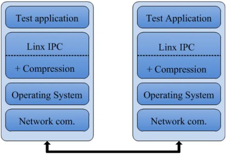
To get a general idea of how and where the actual compres-sion and decomprescompres-sion was performed we needed to famil-iarize ourselves with the provided communication framework by analysing the source code. We were provided with an early prototype that already had LZFX integrated, which gave us a general idea on how to integrate the other al-gorithms. The source code for the selected algorithms was analysed and edited to fit the provided communication frame-work. The compression and decompression was integrated directly into the LINX library as an extra layer to extend the functions that are handling the Inter-Process Communi-cation, as seen in Figure 2. The test application then used the LINX library to send IPC messages between the sender and receiver. The sender, called pong, compresses a mes-sage (if compression is selected) and sends the mesmes-sage to the receiver, called ping, which decompresses the message followed by immediately compressing the message again and
sending it back to pong. Before sending the message, pong adds the current time to the message header. When the transfer was complete the application used this timestamp to calculate the Round-trip Time (RTT) of the message. We added a global variable in the LINX library that contained the compression ratio, which was used by pingpong to calcu-late the average compression ratio for consecutive messages compressed with the same algorithm as well as printing it out to the user. The message flow can be seen in Figure 2.
Figure 2: Message flow with compression as an extra layer in LINX
7.1
Test cases
The real telecom message data was exported from a Wire-shark8 log. While analysing the Wireshark log, we noticed
that the messages were sent with a throughput of 14 Mbit/s. This could be because the bandwidth was low or the network load was high. However, we had 10, 100 and 1000 Mbit/s dedicated throughput when our tests were performed, i.e. no other traffic was present. Together with this informa-tion and the factors in Secinforma-tion 6 on the preceding page, we constructed the test cases that can be seen below.
For 10, 100, and 1000 Mbit/s network bandwidth
– Send 5000, 10000 and 20000 messages, respectively, with telecom signal data of size 500, 700, 1000 and 1400 byte
– Compress and decompress the messages with LZO, LZFX, LZMA, bzip2, LZW, LZ4 and without com-pression
– Acquire the average round-trip time and compression ratio
– Calculate the effective throughput using the average round-trip time
Note that there was only one concurrent message on the network at any given time, i.e. we do not send a stream of messages. This means that one message was sent and the next message was not sent until the previous message returned.
As a last test we determined the maximum throughput for our application by sending many large messages over a long period of time while at the same time monitoring the through-put using iftop. This was done to see if we could utilize one hundred percent of the maximum available bandwidth. To verify that the available bandwidth was correct we used iperf in TCP mode. We used TCP mode since we use LINX with TCP connections.
7.2
Data working set
The data set used in the experiments was taken from a dump of traffic data that was acquired by sniffing the traffic of a node in a real telecom network. From this dump, 100 packets were exported as static arrays to a C header file using Wireshark. The exported packets were not filtered for any specific senders or receivers. To fill the payload of the messages in our experiment, we looped through the arrays in the header file and copied the data. Initial test runs showed that the protocol header of each packet could be compressed to a higher degree than the payload of the packet. Because of this, we excluded the headers of the packets to give the worst-case scenario. The total amount of data, excluding protocol headers, was approximately 20kB.
7.3
Formulas for effective throughput
In our experiment, the throughput B is defined as B =Dc
t (3)
where Dcis the size of the compressed data and t is the time
required to send that data between the two nodes. This means the time to compress and uncompress the data is also included in t. While running the tests for a specific bandwidth, B should be constant and Dcand t should vary
depending on the compression algorithm used.
The effective throughput Be, also called goodput, is defined
as
Be=
D
t (4)
where D is the size of the data before compression and t is the same as in Equation (3). In our tests D will be constant. If we use no compression, the compressed size of the data Dc will be equal to the size of the noncompressed data D,
which means that by using Equation (3) and Equation (4), we get B = Be in the case of sending noncompressed data.
To calculate the change in effective throughput from using some compression algorithm A, we calculate the quotient QA
between BeA and B, where BeA is the effective throughput for algorithm A QA= BeA B = D/tA D/tU C =⇒ Q = tU C tA (5) Here, tA is the time when using algorithm A and tU C is
the time when sending noncompressed data. The effective throughput for algorithm A will then be
BeA= QAB = tU C
tA
B (6)
8.
IMPLEMENTATION
In this section we describe how we setup the test environ-ment and impleenviron-mented the compression algorithms chosen.
8.1
Test environment
The test environment is shown in Figure 3 where the “Con-trol Network” is the network to access the servers where the tests were done. The connection between server 1 and 2, called “Data Network” in Figure 3, is where the communi-cation was done. The “Data Network” is where we config-ured the bandwidth by setting the link speed on the servers, while the link speed of the switch remained the same in all tests. We also tested how the performance is affected when removing the switch between the servers and connect-ing them point-to-point. Both networks have 1000 Mbit/s network capacity. The servers have all the software needed to perform the tests. This includes a test program that sends noncompressed and compressed LINX IPC messages using the selected compression algorithms as seen in Fig-ure 2 on the previous page. The servers runs Ubuntu Linux 12.10 (Quantal Quetzal) with kernel version 3.5.0-28-generic x86 64. The specification of the server hardware can be seen in Table 6.
Figure 3: Hardware setup used in the tests
CPU 2 x AMD Opteron® 6128 2.00 GHz
- Physical cores per CPU: 8 - Max threads per CPU: 8
- L1 instr. cache per CPU: 8 × 64 kB - L1 data cache per CPU: 8 × 64 kB - L2 Cache per CPU: 8 × 512 kB - L3 Cache per CPU: 2 × 6 MB
Memory Samsung DDR3 32 GB
- Clock Speed: 1333 MHz
HDD Seagate 250 GB
- RPM: 7200
- I/O transfer rate: 300 MB/s - Cache: 8 MB
NIC Intel 82576 Gigabit Network Connection - Data rate: 10/100/1000 Mbps
- Number of ports: 2
8.2
Compression algorithms
The algorithms were integrated directly into the LINX li-brary, more specifically into ../liblinx/linx.c. The method linx_send_w_s has been extended to compresses the mes-sages with the selected algorithm while the linx_receive method handles the decompression. In these methods the RTT and compression ratio were also calculated. The test application, pingpong, that uses the LINX library to send and receive messages was used to select which compression algorithm to use, how many messages that should be sent, the content and size of each message and where to send the messages. Here we also calculated the average RTT and the average compression ratio. pingpong also fills the message payload with data. In our case we call the func-tion fill_buffer where the first parameter fill_method determines which method to use. One of the methods is to use real telecom data by calling the function init_buffer-_from_pkts, which is implemented in pkt1_to_100.h. This function fills the payload buffer with real telecom data as described in Section 7.2 on the preceding page.
8.2.1 LZO
The source code used for LZO was taken from the offi-cial website [61]. We used the lightweight miniLZO version since all that was needed was the compress and decompress functions. The files minilzo.c, minilzo.h, lzodefs.h and lzoconf.h were included directly into ../liblinx/linx.c. Compression was then done by using the lzo1x_1_compress function, while decompression was done by using the lzo1x_-decompress function. Both functions take pointers to the in-put and outin-put buffers, as well as the size of the inin-put buffer by value and the size of the output buffer as a pointer. The number of bytes written to the output buffer will be written to the address of the output buffer pointer when the func-tion returns. The compression funcfunc-tion also takes a pointer to a memory area that is used as working memory. The size of the working memory used was the default size.
8.2.2 LZFX
For LZFX, we used the source code found on [63]. The files lzfx.c and lzfx.h were included in ../liblinx/linx.c without any modifications. Compression and decompres-sion was then performed by calling the lzfx_compress and lzfx_decompress methods, respectively. Pointers to the in-put and outin-put buffers are passed to both the decompress and compress functions. The size of the input buffer is sent by value, while the size of the output buffer is sent as a pointer. When the functions return, the number of bytes written to the output buffer is stored in the address of this pointer.
8.2.3 LZW
The source code used for LZW is based on M. Nelson’s ex-ample source code which was modified in 2007 by B. Banica to use buffers instead of files [66]. To be able to use the code in our application we made the following changes:
– Modified the source to work without the main-method so that we could use the encode and decode method di-rectly, this was done by moving the memory allocation into encode and decode.
– Changed the interface for encode and decode to take a pointer to the output buffer and the size of the buffer instead of allocating the buffer in the functions.
– Made the function calls re-entrant by replacing most of the static variables with function parameters. – Added checks to avoid reading or writing outside the
buffers and some small optimizations.
– Change the way fatal errors was handled by returning a value instead of terminating the application. Zero means the execution was successful, negative one in-dicates that the output buffer was too small or the compressed size was larger than the original size and negative two are fatal errors which terminates our test application.
LZW does not take any other arguments, however it is pos-sible to redefine the number of bits used for the code-words by changing the value of the BITS constant. We did some test runs and came to the conclusion that 9 bits was optimal for our data.
8.2.4 LZMA
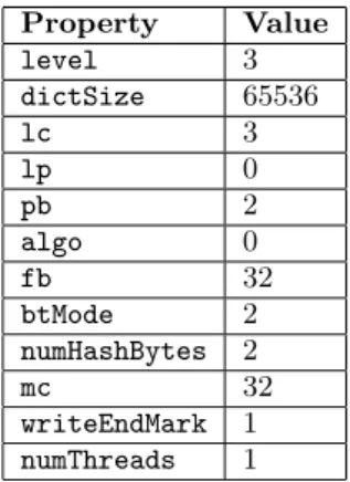
The source code used for LZMA was the one included in the LZMA SDK version 9.20 by 7-zip [53]. The files needed to compress and decompress using LZMA were: LzFind.c, LzFind.h, LzHash.h, LzmaDec.c, LzmaDec.h, LzmaEnc.c, Lz-maEnc.h and Types.h. To compress and decompress mes-sages the methods LzmaEncode and LzmaDecode were used. LzmaEncode required additional properties to determine how the compression would be done, e.g. dictionary size, com-pression level, whether to use an end-mark or not etc. When calling LzmaDecode the properties used when encoding must be known. We chose to insert the properties in the begin-ning of each message. We performed some test runs with real telecom data to determine appropriate values for each property. The values we selected can be seen in Table 7.
Property Value level 3 dictSize 65536 lc 3 lp 0 pb 2 algo 0 fb 32 btMode 2 numHashBytes 2 mc 32 writeEndMark 1 numThreads 1
Table 7: LZMA encode and decode properties
8.2.5 bzip2
To integrate bzip2 we used version 1.0.6 of the library lib-bzip2 [51], which we compiled and installed on the sys-tem. Encode and decode methods were implemented into linx.c and the libbzip2 library is linked in when building the LINX library as well as the test application pingpong. The block size for compression was set to the smallest pos-sible value, 100 kB, since the size of the messages that were compressed is at most a few kilobytes. The workFactor pa-rameter is used to determine when to use a slower, but more deterministic, fallback algorithm. We tested different values
for this parameter on the real telecom data, but saw no dif-ference. This should mean the data we used is not near the worst-case, because the fallback algorithm is only used for worst-case data. We therefore used the default value. In the decompress function, the small parameter is used to switch to a slower algorithm that uses at most 2300 kB of memory. Since the literature study showed that fast algorithms were to prefer, we used the faster version of the function with higher memory requirements.
8.2.6 LZ4
We used the official source code for LZ4 made by Y. Col-let [50]. We decided to use the normal version of LZ4 and not the threaded version since we did not use multi-threading support for the other algorithms. Some of them did not even have support for multi-threading, thus mak-ing it more fair. The files needed to integrate LZ4 were lz4.c, lz4.h, lz4_decode.h and lz4_encode.h. We did not need to change the source code at all, we simply call the LZ4_compress and LZ4_decompress_safe methods for compressing and decompressing. Pointers to the input and output buffers were passed to these functions, as well as an integer specifying the size of the input data. The de-compression function also takes an argument that specifies the maximum size of the output buffer, while it is assumed in the compression function that the output buffer is of at least the same size as the input buffer. Both functions re-turns the number of bytes written to the output buffer, in case of success. In order to avoid stack overflow, we needed dynamic memory allocation and therefore changed the value of HEAPMODE to 1.
9.
RESULTS
The results from the tests when using a switch on the data network can be seen in Figure 4, 5 and 6, while the mea-surements from the point-to-point connection can be seen in Figure 7, 8 and 9. All the measurements were calculated ac-cording to Equation (6) on page 12. The lines represents the average effective throughput for one concurrent mes-sage when using the different compression algorithms and no compression. The available link speed can be seen at the top of each figure, which is also the theoretical imum throughput. As a final test we measured the max-imum throughput for the test application as described in Section 7.1 on page 11. The result of this test can be seen in Table 8.
Connection type Maximum Throughput
Switched 261 Mbit/s
Point-to-point 265 Mbit/s
Table 8: Maximum throughput for the test applica-tion with point-to-point and switched connecapplica-tion.
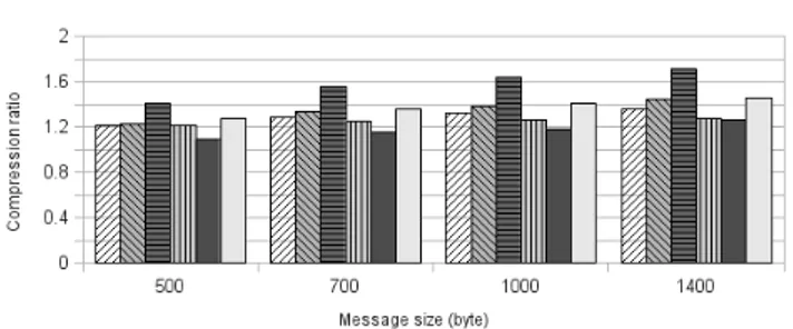
Figure 10 shows the average compression ratio for all the algorithms used when compressing LINX IPC messages of size 500, 700, 1000 and 1400 byte.
10.
CONCLUSION
When compressing LINX IPC messages, some factors had impact on whether it was beneficial or not, in terms of ef-fective throughput. If the time spent on transferring the messages was high, compared to the time spent compress-ing and decompresscompress-ing the messages, an increase in efficient
network throughput could be achieved. Regardless of if the time spent transferring the messages depends on low net-work bandwidth or a high number of hops, the compression and decompression time will be such a small part of the total transfer time that it will be profitable to use compression. This means that the choice of algorithm depends on the size of the messages, as well as the properties of the network, such as the complexity and available bandwidth. In our case the fastest algorithms, that still achieved a relatively high compression ratio, were best suited. This was also the conclusion we made from the literature study.
LZ4 and LZO performs almost equally and are the most effective of all the algorithms we tested. They are both de-signed to be very fast, just as LZFX. However, LZFX is always a few steps behind both LZ4 and LZO, and this gap seems to increase with higher link speed. This could be the effect of lower compression ratio, as seen in Figure 10 on page 16, or possibly slightly longer compression and decom-pression time. LZ4 was slightly better than LZO, most of the time achieving a few percent higher effective throughput, and in worst case performing equal to LZO.
The performance of LZW is low because the compression ratio does not increase much when the size of the message increases, compared to other algorithms. This is probably because we chose to use a low number of bits for the code-words, due to the small size of the messages.
LZMA achieved the highest compression ratio of all the tested algorithms, but since the compression and decom-pression time was high, we did not see any improvement of the effective throughput. However, what we can see was that LZMA gained more than the other algorithms from increased complexity in the network, which means that it might be the most beneficial algorithm in more complex net-works.
bzip2 was the worst of the algorithms tested since it had too low compression ratio compared to the other algorithms. The compression and decompression time was also the longest of all algorithms.
Looking back at Table 5 on page 10 the predictions were correct for LZO, LZFX, LZMA and LZ4. bzip2 seemed to have a longer execution time than LZMA and the compres-sion ratio was very low, while we expected it to be high. The achieved compression ratio for LZW was also lower than we had expected.
As discussed in Section 6 on page 10, the compression might become a bottleneck when transferring messages. When the link speed was set to 1000 Mbit/s, regardless of whether we used point-to-point or switched connection, we got negative effects when using any of the compression algorithms. In table 8 we can see that the maximum throughput for the test application was around 260 Mbit/s, which means that we never used the maximum available throughput when the link speed was set to 1000 Mbit/s. However, the through-put was approximately 14 Mbit/s when analysing the logs for real telecom traffic. This means it should be beneficial to use compression in the real environment since we saw improvement on bandwidths up to 100 Mbit/s.
Figure 4: Average effective throughput per message using various algorithms with 10 Mbit/s link speed and a switched network.
Figure 5: Average effective throughput per message using various algorithms with 100 Mbit/s link speed and a switched network.
Figure 6: Average effective throughput per mes-sage using various algorithms with 1000 Mbit/s link speed and a switched network.
Figure 7: Average effective throughput per message using various algorithms with 10 Mbit/s link speed.
Figure 8: Average effective throughput per message using various algorithms with 100 Mbit/s link speed.
Figure 9: Average effective throughput per mes-sage using various algorithms with 1000 Mbit/s link speed.