Does uncertainty make cost-benefit analyses pointless?
Disa Thureson1 and Jonas Eliasson2 1Division of Transport Economics,
The Swedish National Road and Transport Research Institute (VTI) and Örebro University School of Business, Sweden
2Department of Transport Science, KTH Royal Institute of Technology
CTS Working Paper 2016:8 Abstract
Cost-benefit analysis (CBA) is widely used in public decision making on infrastructure investments. However, the demand forecasts, cost estimates, benefit valuations and effect assessments that are conducted as part of CBAs are all subject to various degrees of uncertainty. The question is to what extent CBAs, given such uncertainties, are still useful as a way to prioritize between infrastructure investments, or put differently, how robust the policy conclusions of CBA are with respect to uncertainties. Using simulations based on real data on national infrastructure plans in Sweden and Norway, we study how investment selection and total realized benefits change when decisions are based on CBA assessments subject to several different types of uncertainty. Our results indicate that realized benefits and investment selection are surprisingly insensitive to all studied types of uncertainty, even for high levels of uncertainty. The two types of uncertainty that affect results the most are uncertainties about investment cost and transport demand. Reducing uncertainty can still be worthwhile, however, because of the huge amounts of money at stake: a 10% reduction in general uncertainty can increase the realized benefits of a national infrastructure investment plan by nearly 100 million euro (assuming that decisions are based on the CBAs). We conclude that, despite the many types of uncertainties, CBA is able to fairly consistently separate the wheat from the chaff and hence contribute to substantially improved infrastructure decisions.
Keywords: Cost-benefit analysis; infrastructure investments; uncertainty; robustness.
JEL codes: R42, R48
Centre for Transport Studies SE-100 44 Stockholm
Sweden
2
1 INTRODUCTION
In public decision making, for example regarding infrastructure investments, CBA is frequently used to systematically compare costs and benefits of various projects. Such analyses are based on forecasts of likely future scenarios, with and without the project in question. These forecasts are obviously subject to uncertainties, and so are the valuations of costs and benefits of the respective projects. Such fundamental uncertainties have led many researchers and policy makers to question the usefulness of CBA as a basis for public decision making. For example, Flyvbjerg (2009) criticizes CBA as a selection criterion based on the lack of precision in forecasts of investment costs and transport demand. He argues that the errors in forecasting are of such magnitude that CBAs will “with a high degree of certainty be strongly misleading,” concluding with the words, “Garbage in, garbage out” (p. 348).
But will this intuitively persuasive argument hold up in reality? In the present study we aim to answer this question by investigating how robust the policy recommendations of CBAs of infrastructure investments are with respect to several kinds of uncertainty. We use a simulation-based approach based on real data to explore how uncertainties affect selection of investments under a given budget, and how they hence affect the total achieved net benefits of the resulting investment portfolio. This is compared with both the ideal selection (under no uncertainty) and a random selection of investments from the list of candidates. The latter comparison represents a choice situation where decisions are made without any consideration of CBA results. In fact, previous research has found that politicians’ investment selections are virtually indistinguishable from random selection from the list of investment candidates, and that the transport administrations’ compilations of investment candidates (which are done before CBAs are made) indicate that it is very difficult, even for professionals, to assess cost-efficiency of investments without CBA results (Eliasson et al., 2015; Eliasson & Lundberg, 2012).
We study the sensitivity of selection and realized total benefits with respect to uncertainties in forecasts of investment costs, transport demand, assessment of effects, and valuations of benefits (travel time savings, freight benefits, traffic safety, and CO2 emissions). We study both systematic and random errors. Data on infrastructure investment CBAs from Sweden and Norway are used to perform the analyses.
Each investment candidate is assumed to have true values of benefits and costs, but the decision maker can only estimate benefits and costs subject to forecasting/measurement errors (which can be systematic or random). The decision maker selects the investments estimated to yield the highest total benefit subject to a budget constraint. This actual selection, based on the estimated costs and benefits, is then compared with the ideal selection, i.e., the one which would actually yield the highest net benefits and which the decision maker would have selected in the absence of the forecasting/measurement errors. We compare actual and ideal selections in terms of both the number of
3
investments that are different and the difference in realized benefits, i.e., the loss in net benefits caused by the uncertainty in benefits and costs.
The analysis consists of two parts. In the first, we examine systematic uncertainty in benefit valuations, i.e., the true valuation of a specific benefit is over- or underestimated for all investments. In the second part, we examine random forecasting errors, i.e., when benefits and costs of each project are estimated subject to errors that differ across projects and that may be different for different types of benefits. We use Monte Carlo simulation for this task, with error distributions of investment costs and travel demand based on Flyvbjerg et al.’s studies (2002, 2005), in order to test whether Flyvbjerg’s claim “garbage in, garbage out” holds in practice. We also study how fast the quality of CBA recommendations deteriorates as total uncertainty increases. This is similar to an analysis by Eliasson and Fosgerau (2013), but in the present study the representation of uncertainty is more detailed.
Sensitivity of CBA ranking to uncertainty has previously been studied by Börjesson et al. (2014) and Holz-Rau and Scheiner (2011). In both cases it was concluded that CBA ranking is fairly robust against the examined uncertainties. These studies only looked at how the ranking was changed, not at the losses in terms of total net benefits that these changes resulted in, which we do in the present study. We show that this methodological difference is important, as the loss in total net benefits is typically significantly more robust against some types of uncertainty. The present study extends the results in Börjesson et al. (2014) and Eliasson and Fosgerau (2013) in several ways; three different datasets are used and compared; investments are selected under a given budget constraint, rather than selecting a fixed number of projects; uncertainty intervals and probability distributions are based on empirical findings; and more types of uncertainty are explored and compared.
The assumption of a fixed investment can of course be questioned. One could argue that the estimated net benefits of potential projects should influence the total size of the investment budget. This may be reasonable in theory, but there is little evidence that it is indeed the case. From this perspective, it seems most realistic to look at ranking and selection decisions under a given budget rather than decisions about the total investment budget.
Our results indicate that selections based on CBA are in fact fairly robust. Selecting investments based on estimated costs and benefits yields much larger total net benefit than random selection from a list of candidates (i.e., disregarding CBA results), even for very high levels of uncertainty. Comparing with a random selection may seem unfair; one might reasonably expect that even if decision makers do not use or trust formal CBAs, there should at least be some correlation between benefits, costs, and decisions. However, this is in fact not the case. Several previous studies have found no or very limited correlation between decisions and measurable benefits and costs (Eliasson et al., 2015; Fridstrøm & Elvik, 1997; Nyborg, 1998; Odeck, 1996, 2010). In other words, it is in fact not uncommon that investment selections are indistinguishable from
4
random selection, from a CBA point of view. Hence, random selection serves as a useful benchmark for assessing the potential gains in total benefit of using CBA. Next section starts with a simple model description and continues with an overview of the most important sources of uncertainty. Section 3 describes the data used in the present study. In Section 4 unit value uncertainty is analyzed and in Section 5 forecast uncertainty is analyzed. The paper ends with some concluding remarks in Section 6.
2 METHODOLOGY
This section starts with a model description, which forms the basis of the analysis in the present paper. Next, the most important sources of uncertainty are described in qualitative terms in relation to the model, through a systematic table (Table 1). We also describe to what extent these different types of uncertainties have been covered in previous studies and how the present study investigates them.
Let qij be effects of different types j resulting from investment 𝑖. The different
types of effects can be for example changes in travel times, emissions, and traffic safety. We will assume that the effects are proportional to transport demand 𝐷𝑖. The monetary benefit 𝐵𝑖𝑗 is the product of the effect and its unit valuation 𝜃𝑗:
𝐵𝑖𝑗 = 𝑞𝑖𝑗∙ 𝜃𝑗.
Note that both 𝑞𝑖𝑗 and 𝜃𝑗 can be either positive or negative. The total benefit of investment 𝑖 is hence:
𝐵𝑖 = ∑ 𝐵𝑖𝑗 𝑗
.
We assume that 𝐵𝑖 ≥ 0 for all 𝑖. Each investment also has an investment cost 𝑐𝑖. The decision maker’s problem is to select an investment portfolio that maximizes total benefits, given a budget constraint C. Letting 𝛿𝑖 be an indicator variable indicating whether investment 𝑖 is selected or not, we can write this problem as: max {𝛿𝑖} ∑ 𝛿𝑖𝜃𝑗𝑞𝑖𝑗 𝑖𝑗 s.t. ∑ 𝛿𝑖𝑐𝑖 𝑖 ≤ 𝐶 𝛿𝑖 ∈ {0,1} ∀𝑖.
The knapsack theorem says that the optimal solution to this maximization problem is to rank all investment candidates according to their benefit/cost ratios 𝐵𝑖/𝑐𝑖 and then select investments according to this ranking until the
5
budget constraint C is met.1 Call the solution to this maximization problem (the optimal investment selection) 𝛿∗= {𝛿
𝑖∗}. Let 𝐵∗ be the net benefit with the optimal investment selection:
𝐵∗ = ∑ 𝛿 𝑖∗[𝜃𝑗𝑞𝑖𝑗 − 𝑐𝑖] 𝑖𝑗 = ∑ 𝛿𝑖∗𝜃 𝑗𝑞𝑖𝑗 𝑖𝑗 − 𝐶,
and define the net benefit/investment cost ratio NBIR* as:
𝑁𝐵𝐼𝑅∗ =𝐵∗ 𝐶.
However, the decision maker can only observe the effects qij, transport demand
𝐷𝑖, the valuations 𝜃𝑗, and the investment costs 𝑐𝑖 subject to uncertainty. Hence, the decision maker selects investments by solving the following optimization problem, conditional on forecasting/measurement errors of effects 𝜀𝑖𝑗𝑞, valuations 𝜀𝑗𝜃, demand 𝜀
𝑖𝐷, and investment cost 𝜀𝑖𝑐: max {𝛿𝑖} ∑ 𝛿𝑖(1 + 𝜀𝑖 𝐷) ∙ (1 + 𝜀 𝑗𝜃)𝜃𝑗∙ (1 + 𝜀𝑖𝑗𝑞)𝑞𝑖𝑗 𝑖𝑗 s.t. ∑ 𝛿𝑖 ∙ (1 + 𝜀𝑖𝑐)𝑐 𝑖 𝑖 ≤ 𝐶 𝛿𝑖 ∈ {0,1} ∀𝑖.
Denote the solution to this problem, i.e., the decision maker’s selection conditional on all the uncertainties, 𝛿 = {𝛿𝑖}. Define the realized net benefits B as:
𝐵 = ∑ 𝛿𝑖[𝜃𝑗𝑞𝑖𝑗 − 𝑐𝑖] 𝑖𝑗
.
B is hence the true net benefit of the investment portfolio selected by the decision maker, conditional on the uncertainty terms.
In our simulations, we use two measures of the consequences of the uncertainty. The first is the share of omitted projects 𝜌𝑝𝑟𝑜𝑗𝑒𝑐𝑡𝑠, defined as the relative number of investments that should have been selected but were not:
1 Note that this formulation tacitly assumes that there is no opportunity cost of money, i.e., there is
no incentive for the decision maker to avoid investments with negative net benefits 𝐵𝑖− 𝑐𝑖 as long
as gross benefits 𝐵𝑖 are positive. This assumption may appear strange but is consistent with the
framing of decision making for public agencies. It is not important for our general conclusions, however, and as long as the total cost for all investments with positive net benefits exceeds the budget constraint, it makes no difference.
6 𝜌𝑝𝑟𝑜𝑗𝑒𝑐𝑡𝑠= 1 −∑ 𝛿𝑖𝛿𝑖 ∗ 𝑖 ∑ 𝛿𝑖∗ 𝑖 .
The second and more important measure is the relative loss in net benefits 𝜌𝑏𝑒𝑛𝑒𝑓𝑖𝑡𝑠, defined as the realized net benefits relative to the maximal achievable net benefits: 𝜌𝑏𝑒𝑛𝑒𝑓𝑖𝑡𝑠 = 1 − 𝐵 𝐵∗ = 1 − ∑ 𝛿𝑖𝑗 𝑖[𝜃𝑗𝑞𝑖𝑗− 𝑐𝑖] ∑ 𝛿𝑖∗[𝜃 𝑗𝑞𝑖𝑗 − 𝑐𝑖] 𝑖𝑗 .
Thus, the relative benefit loss caused by the uncertainties is 𝐵𝐵∗− 1.
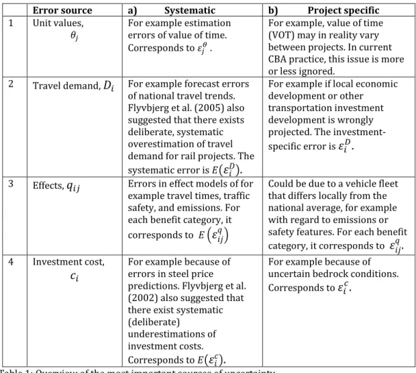
In the following, we will specify the uncertainties in several different ways. The most important sources of uncertainty are summarized in Table 1. Note that each uncertainty can be either systematic or investment specific.
Error source a) Systematic b) Project specific
1 Unit values, 𝜃𝑗
For example estimation errors of value of time. Corresponds to 𝜀𝑗𝜃 .
For example, value of time (VOT) may in reality vary between projects. In current CBA practice, this issue is more or less ignored.
2 Travel demand, 𝐷𝑖 For example forecast errors of national travel trends. Flyvbjerg et al. (2005) also suggested that there exists deliberate, systematic overestimation of travel demand for rail projects. The systematic error is 𝐸(𝜀𝑖𝐷).
For example if local economic development or other transportation investment development is wrongly projected. The investment-specific error is 𝜀𝑖𝐷.
3 Effects, 𝑞𝑖𝑗 Errors in effect models of for example travel times, traffic safety, and emissions. For each benefit category, it corresponds to 𝐸 (𝜀𝑖𝑗𝑞)
Could be due to a vehicle fleet that differs locally from the national average, for example with regard to emissions or safety features. For each benefit category, it corresponds to 𝜀𝑖𝑗𝑞.
4 Investment cost,
𝑐𝑖 For example because of errors in steel price predictions. Flyvbjerg et al. (2002) also suggested that there exist systematic (deliberate)
underestimations of investment costs. Corresponds to 𝐸(𝜀𝑖𝑐).
For example because of uncertain bedrock conditions. Corresponds to 𝜀𝑖𝑐.
Table 1: Overview of the most important sources of uncertainty.
There are two basic types of errors: forecasting errors (rows 3–4 in Table 1), which relate to a quantity, and unit valuation errors (row 1 in Table 1), which relate to monetary valuation of the quantities. Errors may be systematic
7
(column a), for example overestimation of a specific type of benefit for all investments, or project specific (column b).
In Börjesson et al. (2014), the consequences of error type 1a and to some extent 1b2 and 2a3 were examined. In the present study, we examine the consequences of 1a, 2a+2b, 3b and 4a+4b. Note that from a practical perspective, an x% error in 1a is equivalent to an x% error in 3a, and a y% error in 1b is equivalent to a y% error in 3b. Thus, from this perspective the present study also indirectly covers 1b and 3a, which means that we to some extent cover all types of errors described in Table 1. But we still think it is important to stringently distinguish between 1 and 3 on a conceptual level.
We also examine the joint consequences of 2a+2b, 3b, 4a+4b and the effect of increasing the general level of uncertainty, similar to the analysis in Eliasson and Fosgerau (2013) but with a more detailed and partly empirically based representation of uncertainty. Another advantage of the present study compared with the previous ones is that the selection setting is more realistic; instead of choosing a fixed number of projects (regardless of project size), projects are selected to fit in a fixed budget.
The analysis is split into two parts, one where unit valuation uncertainty 𝜀𝑗𝜃 is investigated, and one where forecast uncertainties (of travel demand 𝜀𝑗𝐷, effects 𝜀𝑖𝑗𝑞, and investment cost 𝜀𝑖𝑐) are investigated. In the first part, the analysis is focused on systematic errors in valuations, i.e., possible disparities in valuations that are equal across projects. The uncertainty is represented by extreme values of 𝜀𝑗𝜃, which means that results are in the form of ranges. In the second part, the influence of the forecast uncertainty of each specific project is investigated, using Monte Carlo simulation. In this part, probability density functions are used for 𝜀𝑖𝑗𝑞, which means that results are in the form of expected values and standard deviations.
2 The effect of more differentiated VOT was examined.
3 The effect of factors important for aggregate demand was examined, for example the effect of a
8
3 DATA
Three different datasets of CBAs of road and railway investments in Sweden and Norway are used, referred to as Sweden 2010, Norway 2012, and Sweden 2014. The years refer to the decision year of each national investment plan. The datasets are described in Table 2.
Sweden 2010 Norway 2012 Sweden 2014
Original data source
Candidates for National Transport Investment Plan for Sweden 2010–21 Candidates for National Road Investment Plan for Norway 2014–23 Candidates for National Transport Investment Plan for Sweden 2014–25
Currency SEK NOK SEK
No. of road projects 398 234 94
No. of rail projects 62 0 0
Total no. of projects 460 234 94
Total cost of all projects 223 240 18
Total cost for projects with Bi>ci 98 86 12
Total NBIR 0.12 -0.09 1.00
Table 2: Descriptive data of the datasets used in the present study. All monetary values in billion SEK or NOK.
The projects in these datasets were shortlisted from a larger pool of potential projects. In other words, these are the projects anticipated to yield the highest net benefit according to planners’ judgment. Despite this, the share in terms of total costs, of projects where benefits actually exceed costs, is less than half in the two Swedish datasets. In the Norwegian dataset, even the total NBIR of the complete list is negative.
Sweden 2010 is essentially the same dataset as the one used in Börjesson et al. (2014), although 19 road projects are excluded because of missing data elements. The Sweden 2014 dataset represents only a fraction of the national investment plan, since relevant information required for the analysis is only available for 94 of the road projects (and none of the rail projects). Also, the projects included are relatively small; although they make up almost half of the total number of projects, they only represent about 10% of the total budget (this is partly because rail projects are typically larger). On the other hand, the budget share on beneficial projects is essentially the same as in the original dataset. In the simulations, budget constraints have been assumed to be equal to the total cost of all investments where benefits exceed costs. For Sweden 2010, this assumption corresponds quite well with the total budget in reality.
9
The distributions of NBIRs for the three datasets are shown in Figure 14. The NBIR distributions of the two Swedish datasets are quite similar, but with a higher share of beneficial projects in 2014.
Figure 1: Distribution of net benefits/investment cost ratios (NBIRs) for each dataset. One bar represents one project
4 UNCERTAINTY IN VALUATION
Mackie et al. (2014) show that there is a considerable spread in valuations of benefits, for example the value of time (VOT), the value of a statistical life (VSL), and the valuation of CO2, in the appraisal guidelines of seven OECD countries (including Sweden but not Norway). This can be interpreted as a rather considerable degree of uncertainty. In this section we will analyze the implication of this uncertainty on CBA.
When it comes to uncertainty in valuations (unit values), we are primarily interested in knowing the consequences if current valuations are misestimated. Therefore, the original datasets are assumed to represent the estimated assessments and figures after uncertainty is added to represent the true (unknown) values.
The value of travel time (VOT), value of freight benefits and costs, value of traffic safety, and value of carbon dioxide emissions (CO2) are examined. Travel times and freight benefits are not available separately in the Norwegian dataset, so their combined value (the consumer surplus) is used instead. CO2 emissions are not available either, so this value is not examined in the Norwegian dataset. We use the variation in benefit valuations from Mackie et al. (2014) as an empirical basis for some reasonable uncertainty intervals for each value category. Mackie et al. do not include freight values though, so for this category we use the largest interval of the other categories (value of a statistical life, VSL).5 Table 3 summarizes the findings in Mackie et al. (2014) along with the values used in the present study:
4 Two outliers have been excluded in order to increase visibility. Sweden 2010 has one outlier
with a NBIR of 13.9 (capacity increase on existing motorway in crowded area in the second largest city). Norway 2012 has one outlier, with a NBIR of -12.0 (due to a low investment cost compared with benefits and operational cost).
5 Freight values should in principle be market based, but these values are highly heterogeneous
and less continuous than private trip values and are therefore hard to estimate, which makes them highly uncertain.
-3 0 3 6 9 Sweden 2010 -1 0 1 2 3 Norway 2012 -5 0 5 10 15 Sweden 2014
10
Mackie et al. (2014) The present study
Min max min max
VOT -10% 36% -25% 50%
VSL -18% 169% -40% 150%
CO2 -91% 0% -91% 133%
Table 3: Variation in valuation for three different benefit categories. All figures are related to the Swedish base case.
In general, the idea in this study is to apply slightly larger intervals than in Mackie et al. There is one obvious exception: the maximum VSL from Mackie et al. is higher than in the present study. The reason for this is that the highest value from Mackie et al. (the U.S. valuation) is an extreme outlier compared with the other countries in the study. Since none of the other countries have a higher CO2 value than Sweden, an upper bound needs to be derived from somewhere else. In this case we use the same upper value as the Swedish Transport Administration uses in sensitivity analyses. It is assumed that the valuation of traffic injuries is proportional to VSL.
Table 4 reports the share of omitted projects (𝜌𝑝𝑟𝑜𝑗𝑒𝑐𝑡𝑠) and relative loss in net benefits (𝜌𝑏𝑒𝑛𝑒𝑓𝑖𝑡𝑠). The first columns for each dataset show results when true valuations are lower than estimated valuations, using the numbers in the min column in Table 3. The second columns for each dataset show results when true valuations are higher than estimated valuations, using the max numbers in Table 3.
Dataset Share of omitted projects (%) Relative loss in net benefits (%) Sw10 No12 Sw146 Sw10 No12 Sw14 Travel time 2.5 1.2 0.0 1.6 0.2 1.2 0.0 0.0 Freight 4.6 3.8 1.6 3.3 1.5 1.9 0.0 0.3 Consumer surplus 8.8 1.4 0.8 0.4 Traffic safety 1.9 15 2.7 12 3.3 11 0.6 2.7 0.1 3.4 0.2 1.8 CO2 (SEK/kg) 0.4 4.9 1.6 0.0 0.1 0.5 0.0 0.0
Table 4: Results of inaccurate valuations for three different datasets in the following order: Sweden 2010, Norway 2012, and Sweden 2014.
The most important conclusion is that the relative loss of net benefits is very small, even for the largest errors in valuation – the loss is at most a few percent, despite the fact that the variation in benefit valuations is large. The share of omitted projects is larger, but still small: the largest value is 15%, but in most cases just a few percent. Put differently, the selection manages to get at least 85% and in most cases more than 95% of the investment selection right. Underestimations of the value of traffic safety are systematically more important than underestimations in the other categories, which is consistent
6 The numbers look odd in that 1.6 occurs three times and 3.3 occurs two times, but this is a random
effect. The reason for this is that there is a quite small dataset, so the exact same quotas (20/60 = 3.3% and 1/63 = 1.6%) have appeared several times at random.
11
with the results in Börjesson et al. (2014). This is partly because the uncertainty interval is large and partly because safety benefits account for a relatively large share of total benefits.
That the variation in omitted projects is larger than the loss in total benefits is of course due to the fact that there are several projects with similar net benefits competing for the last spaces in the selection. From a total net benefit point of view, it is not very important which of these are included, which is why the total net benefit is even more robust to uncertainty than the investment selection is. These numbers can be compared with the loss in net benefits resulting from random selection, which varies from 40% to 120% (see Figure 2). (The loss can be larger than 100% because some investments have negative net benefits.) Compared with this, it is clear that using the results of CBA as a selection criterion is immensely better than disregarding them, despite the uncertainties in valuations.
5 FORECAST UNCERTAINTY
In this section the effects of project-specific forecast uncertainty (rows 1–3 in Table 1) are investigated using Monte Carlo simulation. In the simulations, we use the costs and benefits of the projects in the datasets as true values, since true values need to be the same across simulations to allow for comparison. In each simulation, project-specific errors {𝜀𝑖𝑗𝑞}, {𝜀𝑖𝐷}, and/or {𝜀
𝑖𝑐} are drawn from a triangular probability distribution. To compare the importance of different kinds of uncertainties, we simulate different types of errors in different simulations. Each simulation is repeated with 10,000 iterations. The following benefit categories, j, (which are a subset of all categories) are investigated: travel time (for private trips, including business travelers), emissions, freight benefits/costs, traffic safety, and emissions. The uncertainties in transport demand and investment costs are analyzed in the same manner.7 The joint effect of all these types of forecast uncertainties is also investigated.
Two levels of uncertainty are used for each category, one with a low rate of uncertainty and one with a high rate of uncertainty. The shape of the probability density function (PDF) is the same in both cases, but the interval sizes and hence the standard deviations are different. The interval size of the low uncertainty PDF is a quarter of the interval size of the high uncertainty PDF. We use the results from Flyvbjerg et al. (2002, 2005) to decide the standard deviations of the probability distributions for transport demand and investment cost.8 Probability distributions for High rate of uncertainty have been
7 In the case of investment cost and travel demand, the probability distributions are based on
empirical data of deviations ex post compared with ex ante. Therefore, in order to achieve a simulation of ex ante estimates, ex post values are divided by the randomly drawn deviation factors.
8 Note that the data in Flyvbjerg et al. (2002, 2005) was not collected in a systematic,
12
constructed with the same means and standard deviations as in Flyvbjerg et al. (2002, 2005), shown in Table 5.
Study Mode No. Obs. increase % Mean deviation % Standard
Investment cost Flyvbjerg et al., 2002 Both 258 27.6* 38.7*
Travel demand Flyvbjerg et al., 2005
Rail 27 -51.4 44.3
Road 183 9.5 28.1
Present study Both 1.7* 36.7*
Table 5: Reported mean and standard deviaton of increases ex post compared with prediction ex ante, of investment costs and travel demand based on two studies of Flyvberg et al. The three first rows report figures taken directly from the original studies. The last row has been calculated from the two preceeding rows; the mean is taken as weighted avarage while the standard deviation requires more advanced but straightforward calculations9. *The asterix
indicates which figures used to construct probability distributions in the present study. For the purpose of this study, all benefits and costs other than investment cost are assumed to be proprotional to travel demand.
The mode and skewness of the distributions are chosen to be similar to the histograms in Flyvbjerg et al. (2002, 200510).11 The mode of Low rate of uncertainty probability density functions has been set to a quarter of the mode in the High rate of uncertainty distribution. This means that the expected increase in the Low rate of uncertainty distribution is one quarter of the expected increase in the High rate of uncertainty distribution.
Probability distributions of effect uncertainty are based on judgment. The High rate of uncertainty probability distribution is a triangular probability density function with minimum = –50%, mode = 0, and maximum = +100%. This results
Nicolaisen and Driscoll (2014) (see their Table 2), Flyvbjerg et al.’s (2005) results seem to be in line with the other literature from that time. However, there seems to be a downward trend in overestimation of rail travel demand, so that the later studies show a lower degree of
overestimation than in Flyvbjerg et al. (2005). This difference is of limited importance for the present study, though, because no separation between rail and road PDFs is made here and a joint PDF is constructed as a weighted mean of the rail and road pdf:s. Because more road projects than rail projects are included in Flyvbjerg et al.’s study, they will play a more dominant role in the new joint PDF. On the other hand, the mean cost overrun for road projects is high compared with other studies according to Table 3 in Lundberg et al. (2011)), which means that uncertainty regarding investment cost may be overestimated in the present study.
9 𝑠 𝑡𝑜𝑡2 =𝑛 1 𝑡𝑜𝑡−1∑ (𝑥𝑖− 𝑥̅𝑡𝑜𝑡) 2 𝑛𝑡𝑜𝑡 𝑖=1 = =𝑛 1 𝑡𝑜𝑡−1(∑ ((𝑥𝑗− 𝑥̅𝑟𝑎𝑖𝑙) − (𝑥̅𝑡𝑜𝑡− 𝑥̅𝑟𝑎𝑖𝑙)) 2 + 𝑛𝑟𝑎𝑖𝑙 𝑗=1 ∑ ((𝑥𝑘− 𝑥̅𝑟𝑜𝑎𝑑) − (𝑥̅𝑡𝑜𝑡− 𝑥̅𝑟𝑜𝑎𝑑)) 2 𝑛𝑟𝑜𝑎𝑑 𝑘=1 ) = =𝑛 1 𝑡𝑜𝑡−1(∑ ((𝑥𝑗− 𝑥̅𝑟𝑎𝑖𝑙) 2 − 2(xj-x̅rail)(𝑥̅𝑡𝑜𝑡− 𝑥̅𝑟𝑎𝑖𝑙) + (𝑥̅𝑡𝑜𝑡− 𝑥̅𝑟𝑎𝑖𝑙)2) + 𝑛𝑟𝑎𝑖𝑙 𝑗=1 ∑𝑛𝑘=1𝑟𝑜𝑎𝑑((𝑥𝑘− 𝑥̅𝑟𝑜𝑎𝑑)2− 2(xk-x̅road)(𝑥̅𝑡𝑜𝑡− 𝑥̅𝑟𝑜𝑎𝑑) + (𝑥̅𝑡𝑜𝑡− 𝑥̅𝑟𝑜𝑎𝑑)2) 2 ) = =𝑛 1 𝑡𝑜𝑡−1((𝑛𝑟𝑎𝑖𝑙− 1)𝑠𝑟𝑎𝑖𝑙 2 + 𝑛 𝑟𝑎𝑖𝑙(𝑥̅𝑟𝑎𝑖𝑙− 𝑥̅𝑡𝑜𝑡) + (𝑛𝑟𝑜𝑎𝑑− 1)𝑠𝑟𝑜𝑎𝑑2 + 𝑛𝑟𝑜𝑎𝑑(𝑥̅𝑟𝑜𝑎𝑑− 𝑥̅𝑡𝑜𝑡))
10 In the demand case, no aggregate histogram of road and rail projects is presented in Flyvbjerg
et al. (2005). Therefore, in the present study, first two proxy probability distributions of road and rail investments are constructed, then a weighted average PDF of those two is taken as a basis for visual judgment of mode (and skewness). From this, a new triangular probability distribution is constructed with the correct mean and standard deviation.
11 The resulting triangular probability density functions (of change ex post compared with ex
ante) are defined as follows: investment cost – min = –57%, mode= 10%, max =130%; travel demand – min = –84.8%, mode= –5%, max = 94.8%.
13
in a standard deviation of 31.2%, which is of the similar order as the probability distributions from Flyvbjerg et al. (2002, 2005).
Results in terms of share of omitted projects and relative loss of net benefits are shown in Table 6.
Dataset Share of omitted projects (%) Relative loss in net benefits (%) Sw10 No12 Sw14 Sw10 No12 Sw14 Travel time 3.7 10 1.3 7.1 0.2 5.3 0.0 0.8 Freight 0.6 2.6 0.0 1.0 0.0 0.6 0.0 0.0 Consumer surplus 3.4 12 0.4 5.2 Traffic safety 1.5 3.9 2.0 4.0 1.8 5.9 0.0 0.4 0.0 0.8 0.0 0.5 Emissions 0.6 2.2 0.0 0.7 0.0 0.0 0.0 0.1 0.0 0.0 0.0 0.0 Travel demand 4.1 17 4.6 20 3.4 13 0.5 15 0.7 12 0.2 2.2 Investment cost 1.7 6.8 1.9 6.2 1.1 2.3 1.5 15 1.1 12 0.2 1.9 All uncertainties 4.4 14 4.3 15 2.7 4.6 3.2 23 2.3 26 0.4 3.0
Table 6: Results of inaccurate project-specific forecasts for three different datasets in the following order: Sweden 2010, Norway 2012, and Sweden 2014. The first and second columns of each dataset denote a low and a high rate of uncertainty, respectively.
For the low level of uncertainty (the left column for each dataset), the effects of the uncertainties are essentially negligible, i.e., never more than a few percent, even for all kinds of uncertainty combined, and in most cases even much less than that.
For the high level of uncertainty, some types of uncertainty matter: uncertainty of travel demand, investment cost, and travel time savings (included in the consumer surplus in the Norway 2012 dataset) matter for the Sweden 2010 and Norway 2012 datasets. Other uncertainties have negligible effects. Even in these cases, however, the loss of net benefits is limited (12–15%), and the share of omitted projects is also relatively low. Combining all uncertainties simultaneously, the loss of net benefits increases to 23–26% for the Sweden 2010 and Norway 2012 datasets. The loss in the Sweden 2014 data set is much smaller, which is because the budget is relatively high compared with the total cost of investments.
The low share of omitted projects when uncertainty about investment cost is included (the last two rows in Table 6) is slightly misleading. The reason is that costs are underestimated on average, according to the probability density functions used, which are based on Flyvbjerg et al. (2002). This also means that too many projects are included, so that the total budget is overdrawn ex post. When the total budget ex post is expanded, the risk of missing a feasible project is decreased, yet the risk of including a non-feasible project is increased. For example, the share missed out projects in the case of high rate of uncertainty for Sweden 2014, given by the last three rows in Table 6, can be compared to the
14
share of non-feasible projects included: 8% for travel demand, 19% for investment cost, and 20% for all uncertainties.
Uncertainty affects the share of omitted projects more than it affects the relative loss in net benefits. That is, total net benefits is robust when it comes to small forecast uncertainties (much more so than the share of omitted projects), but less so for very large uncertainties. The reason for this is that because there is a great diversion between projects in terms of NBIR, a small uncertainty will not be able to push out good projects; hence robustness will be high for small uncertainties. At the same time, great diversity means that stakes are high. If good projects are pushed out in favor of bad projects, due to large inaccuracies resulting from highly uncertain forecasts, the consequences in terms of total net benefits will be high.
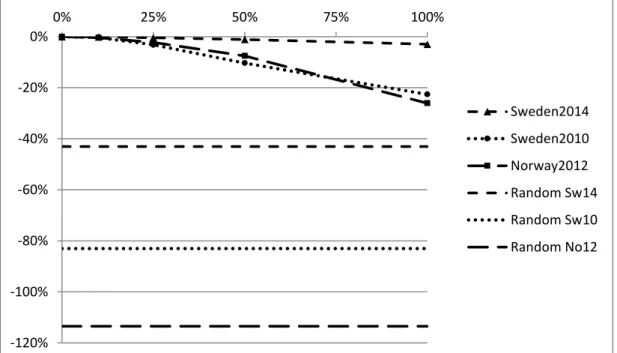
Next, we look at how the relative loss in net benefits changes as overall uncertainty (last row in Table 6) increases. That is, we use the same PDFs as before but gradually expand the interval size from zero to 100% of the interval sizes used in High level of uncertainty analyses. Four simulations are made for each dataset, with different interval of the probability distribution for each simulation: +10%, +25%, +50%, and +100%. The results are shown in Figure 2.
Figure 2: Decrease in total net benefits as a function of total rate of uncertainty, corresponding to the last row in Table 6.
The horizontal axis specifies the degree of uncertainty, as a share of interval size of the High rate of uncertainty pdf in Table 5, and the vertical axis specifies the relative loss in net benefits. The horizontal lines correspond to the loss that would be caused by selecting investments at random.
Although the loss due to uncertainty is significant in the maximum uncertainty case for two of the datasets, the losses are small compared with the losses associated with a random selection. The dataset with the smallest losses due to
-120% -100% -80% -60% -40% -20% 0% 0% 25% 50% 75% 100% Sweden2014 Sweden2010 Norway2012 Random Sw14 Random Sw10 Random No12
15
uncertainty (Sweden 2014) also has the lowest loss from random selection, or conversely, the smallest gain from using CBA ranking as selection criterion instead of a random selection process.
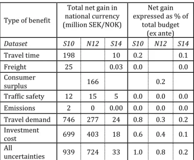
This is not to say that it does not pay off to increase the certainty of cost and benefit estimates. Table 7 shows how total net benefits increase when various types of uncertainty are decreased by 10%, in absolute numbers and relative to the total budget. Since so much money is spent on infrastructure, the potential for increased certainty to yield benefits is also high.
Type of benefit
Total net gain in national currency (million SEK/NOK) Net gain expressed as % of total budget (ex ante) Dataset S10 N12 S14 S10 N12 S14 Travel time 198 10 0.2 0.1 Freight 25 0.03 0.0 0.0 Consumer surplus 166 0.2 Traffic safety 12 15 5 0.0 0.0 0.0 Emissions 2 0 0.00 0.0 0.0 0.0 Travel demand 746 277 24 0.8 0.3 0.2 Investment cost 699 403 18 0.6 0.4 0.1 All uncertainties 939 724 33 1.0 0.8 0.2
Table 7: The implied benefits of a 10% reduction in interval size on an intermediate level of uncertainty (to reduce interval size from 50% to 45% of High rate of uncertainty).12
First, the total gain in benefits is expressed in absolute numbers. In addition, in order to facilitate comparison between countries and relate the figures to something that is certain, it is also presented as share of budget ex ante.
Note that the absolute gain corresponds to different types of pools of projects for the different datasets. Sweden 2010 roughly corresponds to the total national infrastructure investment plan, Norway 2012 roughly corresponds to the national road investment plan, and Sweden 2014 corresponds only to a small subsample of the total investment plan.
One can see that although potential gains are quite modest in share, they are considerable in terms of absolute numbers (for example 939 million SEK is equal to roughly 100 million EUR). This is because total infrastructure investment budgets are typically large.
12 For investment cost, the probability functions with the new, intermediate level of uncertainty
result in expected cost overruns of 13.8%, which is similar to a recent Swedish figure of mean cost overruns of 15.0% (weighted average based on Table 3 in Lundberg et al., 2011). However, standard deviations in Lundberg et al. (2011) were of the same magnitude as in Flyvbjerg et al. (2002), which implies that the benefits of reducing uncertainty may be underestimated in the present study.
16
6 CONCLUSIONS
In the present study we have asked whether uncertainties as regards true costs and benefits of infrastructure investments distort policy recommendations of CBA to an extent that makes them unsuitable for use in decision making. In summary, our results show that uncertainties with regard to valuations and effects cause negligible losses of total net benefits, while the losses caused by project-specific uncertainties regarding investment costs and transport demand matter more, but nowhere near the point at which CBA results become useless or misleading. For the two Swedish datasets, even at the highest uncertainty levels, investment selections based on CBA still achieve realized net benefits that are 70% respective almost five times larger than those of the randomly selected portfolios for each dataset. For the Norwegian dataset, the random selection is too unprofitable for such a comparison to be made, since total net benefits are negative. In the Norwegian case, random selection implies a social loss of 9% of invested capital, whereas the CBA-selected portfolio implies a 110% social return (i.e., the invested capital is more than doubled in terms of value).
One important finding of the present study (in line with results from Eliasson and Fosgerau, 2013) is that, according to Figure 2, potential losses due to uncertainty are small compared with the potential gains of using CBA ranking as selection criterion. Figure 2 also indicates that larger losses due to uncertainty may be correlated with higher gains of using CBA. To use CBA is to utilize variation between projects, and Eliasson and Fosegerau (2013) showed that the higher the variation, the larger the potential gain of using CBA. In the present study we have shown that even when using probability distributions based on the results from Flyvbjerg et al. (2002, 2005), the merit of CBA is not overthrown, in contrast to the claims made in Flyvbjerg (2009). An alternative viewpoint to Flyvbjerg’s could be that in cases with a lot of garbage, it is good to have a filter.
This of course does not mean that suggestions for improvements should not be welcomed. The present study shows that a 10% uniform reduction in uncertainty may yield a 0.2–1% gain as share of budget (last row in Table 7). Because national infrastructures are typically large, these seemingly modest gains add up to large total numbers. In the Swedish case, for example, the potential gain of 1% is equal to 900 million SEK, or roughly around 100 million euro.
However, potential gains are conditional on CBA rankings actually being used as the main criterion for portfolio selection. Eliasson et al. (2015) showed that CBA only partly influences decisions in Sweden and not at all in Norway.13 The present paper, along with others, shows that the greatest potential to increase the quality of infrastructure investment decision may exist in using CBA ranking more consistently.
13It is uncertain to what degree CBA influences decisions also in the United Kingdom, as benefit/cost
17
When it comes to forecast uncertainty, the results indicate that travel demand and investment costs are most important to focus on, and that considerable gains in absolute numbers can be achieved by improving these two types of forecasts. It is also worth noting that systematic errors in investment costs are especially important in that they will lead to a total investment cost that is different from the total budget if no revisions of project plans are made.
REFERENCES
Börjesson, M., Eliasson, J., & Lundberg, M. (2014). Is CBA ranking of transport investments robust? Journal of Transport Economics and Policy, 48(2), 189–204.
Eliasson, J., Börjesson, M., Odeck, J., & Welde, M. (2015). Does Benefit–Cost Efficiency Influence Transport Investment Decisions? Journal of Transport Economics and Policy, 49(3), 377–396.
Eliasson, J., & Fosgerau, M. (2013). Cost overruns and benefit shortfalls - deception or selection? Transportation Research B, 57, 105–113.
Eliasson, J., & Lundberg, M. (2012). Do Cost–Benefit Analyses Influence Transport Investment Decisions? Experiences from the Swedish Transport Investment Plan 2010–21. Transport Reviews, 32(1), 29–48. Flyvbjerg, B. (2009). Survival of the unfittest: why the worst infrastructure gets
built—and what we can do about it. Oxford Review of Economic Policy, 25(3), 344–367.
Flyvbjerg, B., Holm, M. S., & Buhl, S. (2002). Underestimating Costs in Public Works Projects: Error or Lie? Journal of the American Planning Association, 68(3), 279–295.
Flyvbjerg, B., Skamris Holm, M. K., & Buhl, S. L. (2005). How (In)accurate Are Demand Forecasts in Public Works Projects?: The Case of
18
Transportation. Journal of the American Planning Association, 71(2), 131– 146.
Fridstrøm, L., & Elvik, R. (1997). The barely revealed preference behind road investment priorities. Public Choice, 92(1/2), 145–168.
Holz-Rau, C., & Scheiner, J. (2011). Safety and travel time in cost-benefit analysis: A sensitivity analysis for North Rhine-Westphalia. Transport Policy, 18(2), 336–346.
Lundberg, M., Jenpanitsub, A., & Pyddoke, R. (2011). Cost overruns in Swedish transport projects (CTS Working Paper No. 2011:11). Centre for Transport Studies, KTH Royal Institute of Technology.
Mackie, P., Worsley, T., & Eliasson, J. (2014). Transport appraisal revisited. Research in Transportation Economics, Appraisal in Transport, 47, 3–18. Nicolaisen, M. S., & Driscoll, P. A. (2014). Ex-Post Evaluations of Demand
Forecast Accuracy: A Literature Review. Transport Reviews, 34(4), 540– 557.
Nyborg, K. (1998). Some Norwegian Politicians’ Use of Cost-Benefit Analysis. Public Choice, 95, 381–401.
Odeck, J. (1996). Ranking of regional road investment in Norway. Transportation, 23(2), 123–140.
Odeck, J. (2010). What Determines Decision‐Makers’ Preferences for Road Investments? Evidence from the Norwegian Road Sector. Transport Reviews, 30(4), 473–494.