Fermi and Swift Observations of GRB 190114C: Tracing the Evolution of High-energy
Emission from Prompt to Afterglow
M. Ajello1 , M. Arimoto2 , M. Axelsson3,4 , L. Baldini5, G. Barbiellini6,7, D. Bastieri8,9, R. Bellazzini10, A. Berretta11, E. Bissaldi12,13, R. D. Blandford14, R. Bonino15,16, E. Bottacini14,17, J. Bregeon18, P. Bruel19, R. Buehler20, E. Burns21,84,
S. Buson22, R. A. Cameron14, R. Caputo21, P. A. Caraveo23, E. Cavazzuti24, S. Chen8,17, G. Chiaro23, S. Ciprini25,26, J. Cohen-Tanugi18, D. Costantin27, S. Cutini28, F. D’Ammando29 , M. DeKlotz30, P. de la Torre Luque12, F. de Palma15, A. Desai1, N. Di Lalla5, L. Di Venere12,13, F. Fana Dirirsa31, S. J. Fegan19, A. Franckowiak20 , Y. Fukazawa32, S. Funk33,
P. Fusco12,13, F. Gargano13, D. Gasparrini25,26, N. Giglietto12,13, R. Gill34, F. Giordano12,13, M. Giroletti29, J. Granot34 , D. Green35, I. A. Grenier36, M.-H. Grondin37, S. Guiriec21,38, E. Hays21, D. Horan19, G. Jóhannesson39,40, D. Kocevski41, M. Kovac’evic’28, M. Kuss10 , S. Larsson4,42,43 , L. Latronico15, M. Lemoine-Goumard37, J. Li20, I. Liodakis14, F. Longo6,7 ,
F. Loparco12,13, M. N. Lovellette44, P. Lubrano28, S. Maldera15 , D. Malyshev33, A. Manfreda5, G. Martí-Devesa45, M. N. Mazziotta13, J. E. McEnery21,46, I. Mereu11,28, M. Meyer14,33, P. F. Michelson14, W. Mitthumsiri47, T. Mizuno48 , M. E. Monzani14, E. Moretti49, A. Morselli25 , I. V. Moskalenko14 , M. Negro15,16, E. Nuss18, N. Omodei14, M. Orienti29,
E. Orlando14,50, M. Palatiello6,7, V. S. Paliya20 , D. Paneque35, Z. Pei9, M. Persic6,51, M. Pesce-Rollins10, V. Petrosian14, F. Piron18, H. Poon32, T. A. Porter14, G. Principe29, J. L. Racusin21 , S. Rainò12,13, R. Rando8,9, B. Rani21, M. Razzano10,85,
S. Razzaque31, A. Reimer14,45, O. Reimer45, F. Ryde4,42, P. M. Saz Parkinson52,53,54, D. Serini12, C. Sgrò10, E. J. Siskind55, G. Spandre10, P. Spinelli12,13, H. Tajima14,56, K. Takagi32, M. N. Takahashi35, D. Tak21,57, J. B. Thayer14, D. J. Thompson21, D. F. Torres58,59 , E. Troja21,46 , J. Valverde19, B. Van Klaveren14, K. Wood60,86, M. Yassine6,7, G. Zaharijas50, B. Mailyan61, P. N. Bhat61, M. S. Briggs61, W. Cleveland62, M. Giles63, A. Goldstein64, M. Hui65 , Christian Malacaria66,67,87 , R. Preece61,
O. J. Roberts64 , P. Veres61, C. Wilson-Hodge65, A. von Kienlin68, S. B. Cenko69,70 , P. O’Brien71, A. P. Beardmore71, A. Lien72,73, J. P. Osborne71, A. Tohuvavohu74, V. D’Elia75,76, A. D’Aì77, M. Perri75,76, J. Gropp78, N. Klingler78 , M. Capalbi79,
G. Tagliaferri80 , M. Stamatikos21,81,82, and M. De Pasquale83
1
Department of Physics and Astronomy, Clemson University, Kinard Lab of Physics, Clemson, SC 29634-0978, USA
2
Faculty of Mathematics and Physics, Institute of Science and Engineering, Kanazawa University, Kakuma, Kanazawa, Ishikawa 920-1192, Japan arimoto@se.kanazawa-u.ac.jp
3
Department of Physics, Stockholm University, AlbaNova, SE-106 91 Stockholm, Sweden
4
Department of Physics, KTH Royal Institute of Technology, AlbaNova, SE-106 91 Stockholm, Sweden
5
Università di Pisa and Istituto Nazionale di Fisica Nucleare, Sezione di Pisa I-56127 Pisa, Italy
6
Istituto Nazionale di Fisica Nucleare, Sezione di Trieste, I-34127 Trieste, Italy
7
Dipartimento di Fisica, Università di Trieste, I-34127 Trieste, Italy
8
Istituto Nazionale di Fisica Nucleare, Sezione di Padova, I-35131 Padova, Italy
9
Dipartimento di Fisica e Astronomia“G. Galilei”, Università di Padova, I-35131 Padova, Italy
10
Istituto Nazionale di Fisica Nucleare, Sezione di Pisa, I-56127 Pisa, Italy
11
Dipartimento di Fisica, Università degli Studi di Perugia, I-06123 Perugia, Italy
12
Dipartimento di Fisica“M. Merlin” dell’Università e del Politecnico di Bari, I-70126 Bari, Italy
13Istituto Nazionale di Fisica Nucleare, Sezione di Bari, I-70126 Bari, Italy 14
W.W. Hansen Experimental Physics Laboratory, Kavli Institute for Particle Astrophysics and Cosmology, Department of Physics and SLAC National Accelerator Laboratory, Stanford University, Stanford, CA 94305, USA;nicola.omodei@stanford.edu
15
Istituto Nazionale di Fisica Nucleare, Sezione di Torino, I-10125 Torino, Italy
16
Dipartimento di Fisica, Università degli Studi di Torino, I-10125 Torino, Italy
17
Department of Physics and Astronomy, University of Padova, Vicolo Osservatorio 3, I-35122 Padova, Italy
18
Laboratoire Univers et Particules de Montpellier, Université Montpellier, CNRS/IN2P3, F-34095 Montpellier, France
19Laboratoire Leprince-Ringuet, École polytechnique, CNRS/IN2P3, F-91128 Palaiseau, France 20
Deutsches Elektronen Synchrotron DESY, D-15738 Zeuthen, Germany
21NASA Goddard Space Flight Center, Greenbelt, MD 20771, USA;donggeun.tak@gmail.com 22
Institut für Theoretische Physik and Astrophysik, Universität Würzburg, D-97074 Würzburg, Germany
23
INAF-Istituto di Astrofisica Spaziale e Fisica Cosmica Milano, via E. Bassini 15, I-20133 Milano, Italy
24
Italian Space Agency, Via del Politecnico snc, I-00133 Roma, Italy
25
Istituto Nazionale di Fisica Nucleare, Sezione di Roma“Tor Vergata,” I-00133 Roma, Italy
26
Space Science Data Center - Agenzia Spaziale Italiana, Via del Politecnico, snc, I-00133, Roma, Italy
27
University of Padua, Department of Statistical Science, Via 8 Febbraio, 2, 35122 Padova, Italy
28
Istituto Nazionale di Fisica Nucleare, Sezione di Perugia, I-06123 Perugia, Italy
29
INAF Istituto di Radioastronomia, I-40129 Bologna, Italy
30
Stellar Solutions Inc., 250 Cambridge Avenue, Suite 204, Palo Alto, CA 94306, USA
31
Department of Physics, University of Johannesburg, P.O. Box 524, Auckland Park 2006, South Africa
32
Department of Physical Sciences, Hiroshima University, Higashi-Hiroshima, Hiroshima 739-8526, Japan
33
Friedrich-Alexander Universität Erlangen-Nürnberg, Erlangen Centre for Astroparticle Physics, Erwin-Rommel-Str. 1, D-91058 Erlangen, Germany
34
Department of Natural Sciences, Open University of Israel, 1 University Road, POB 808, Ra’anana 43537, Israel;rsgill.rg@gmail.com 35
Max-Planck-Institut für Physik, D-80805 München, Germany
36
AIM, CEA, CNRS, Université Paris-Saclay, Université Paris Diderot, Sorbonne Paris Cité, F-91191 Gif-sur-Yvette, France
37Centre d’Études Nucléaires de Bordeaux Gradignan, IN2P3/CNRS, Université Bordeaux 1, BP120, F-33175 Gradignan Cedex, France 38
The George Washington University, Department of Physics, 725 21st Street, NW, Washington, DC 20052, USA
39
Science Institute, University of Iceland, IS-107 Reykjavik, Iceland
40
Nordita, Royal Institute of Technology and Stockholm University, Roslagstullsbacken 23, SE-106 91 Stockholm, Sweden
41NASA Marshall Space Flight Center, Huntsville, AL 35808, USA;daniel.kocevski@nasa.gov
The Astrophysical Journal, 890:9 (19pp), 2020 February 10 https://doi.org/10.3847/1538-4357/ab5b05 © 2020. The American Astronomical Society.
42
The Oskar Klein Centre for Cosmoparticle Physics, AlbaNova, SE-106 91 Stockholm, Sweden
43School of Education, Health and Social Studies, Natural Science, Dalarna University, SE-791 88 Falun, Sweden 44
Space Science Division, Naval Research Laboratory, Washington, DC 20375-5352, USA
45
Institut für Astro- und Teilchenphysik, Leopold-Franzens-Universität Innsbruck, A-6020 Innsbruck, Austria
46
Department of Astronomy, University of Maryland, College Park, MD 20742, USA
47
Department of Physics, Faculty of Science, Mahidol University, Bangkok 10400, Thailand
48
Hiroshima Astrophysical Science Center, Hiroshima University, Higashi-Hiroshima, Hiroshima 739-8526, Japan
49
Institut de Física d’Altes Energies (IFAE), Edifici Cn, Universitat Autònoma de Barcelona (UAB), E-08193 Bellaterra (Barcelona), Spain
50
Istituto Nazionale di Fisica Nucleare, Sezione di Trieste, and Università di Trieste, I-34127 Trieste, Italy
51
Osservatorio Astronomico di Trieste, Istituto Nazionale di Astrofisica, I-34143 Trieste, Italy
52Santa Cruz Institute for Particle Physics, Department of Physics and Department of Astronomy and Astrophysics, University of California at Santa Cruz, Santa
Cruz, CA 95064, USA
53
Department of Physics, The University of Hong Kong, Pokfulam Road, Hong Kong, People’s Republic of China
54
Laboratory for Space Research, The University of Hong Kong, Hong Kong, People’s Republic of China
55
NYCB Real-Time Computing Inc., Lattingtown, NY 11560-1025, USA
56
Solar-Terrestrial Environment Laboratory, Nagoya University, Nagoya 464-8601, Japan
57
Department of Physics, University of Maryland, College Park, MD 20742, USA
58
Institute of Space Sciences(CSICIEEC), Campus UAB, Carrer de Magrans s/n, E-08193 Barcelona, Spain
59
Institució Catalana de Recerca i Estudis Avançats(ICREA), E-08010 Barcelona, Spain
60
Praxis Inc., Alexandria, VA 22303 USA
61
Center for Space Plasma and Aeronomic Research(CSPAR), University of Alabama in Huntsville, Huntsville, AL 35899, USA;peter.veres@uah.edu 62
Universities Space Research Association(USRA), Columbia, MD 21044, USA
63
Jacobs Technology, Huntsville, AL 35806, USA
64
Science and Technology Institute, Universities Space Research Association, Huntsville, AL 35805, USA
65
NASA Marshall Space Flight Center, Huntsville, AL 35812, USA
66
NASA Marshall Space Flight Center, NSSTC, 320 Sparkman Drive, Huntsville, AL 35805, USA
67
Universities Space Research Association, NSSTC, 320 Sparkman Drive, Huntsville, AL 35805, USA
68
Max-Planck Institut für extraterrestrische Physik, D-85748 Garching, Germany
69
Astrophysics Science Division, NASA Goddard Space Flight Center, 8800 Greenbelt Road, Greenbelt, MD 20771, USA
70
Joint Space-Science Institute, University of Maryland, College Park, MD 20742, USA
71
School of Physics and Astronomy, University of Leicester, University Road, Leicester, LE1 7RH, UK
72
Center for Research and Exploration in Space Science and Technology(CRESST) and NASA Goddard Space Flight Center, Greenbelt, MD 20771, USA
73
Department of Physics, University of Maryland, Baltimore County, 1000 Hilltop Circle, Baltimore, MD 21250, USA
74
Department of Astronomy and Astrophysics, University of Toronto, 50 St. George Street, Toronto, Ontario, M5S 3H4 Canada
75
ASI Space Science Data Center, via del Politecnico snc, I–00133, Rome Italy
76INAF-Osservatorio Astronomico di Roma, via Frascati 33, I–00040 Monte Porzio Catone, Italy 77
INAF-IASF Palermo, via Ugo La Malfa 156, I–90123 Palermo, Italy
78
Department of Astronomy and Astrophysics, 525 Davey Lab, The Pennsylvania State University, University Park, PA 16802, USA
79
INAF-Istituto di Astrofisica Spaziale e Fisica Cosmica di Palermo, Via Ugo La Malfa 153, I–90146 Palermo, Italy
80INAF-Osservatorio Astronomico di Brera, via Bianchi 46, I–23807 Merate (LC), Italy 81
Department of Physics and Center for Cosmology and Astro-Particle Physics, Ohio State University, Columbus, OH 43210, USA
82
Department of Astronomy, Ohio State University, Columbus, OH 43210, USA
83
Department of Astronomy and Space Sciences, Istanbul University, Fatih, 34119, Istanbul, Turkey Received 2019 September 18; revised 2019 November 19; accepted 2019 November 22; published 2020 February 6
Abstract
We report on the observations of gamma-ray burst(GRB) 190114C by the Fermi Gamma-ray Space Telescope and the Neil Gehrels Swift Observatory. The prompt gamma-ray emission was detected by the Fermi GRB Monitor (GBM), the Fermi Large Area Telescope (LAT), and the Swift Burst Alert Telescope (BAT) and the long-lived afterglow emission was subsequently observed by the GBM, LAT, Swift X-ray Telescope(XRT), and Swift UV Optical Telescope. The early-time observations reveal multiple emission components that evolve independently, with a delayed power-law component that exhibits significant spectral attenuation above 40 MeV in the first few seconds of the burst. This power-law component transitions to a harder spectrum that is consistent with the afterglow emission observed by the XRT at later times. This afterglow component is clearly identifiable in the GBM and BAT light curves as a slowly fading emission component on which the rest of the prompt emission is superimposed. As a result, we are able to observe the transition from internal-shock- to external-shock-dominated emission. We find that the temporal and spectral evolution of the broadband afterglow emission can be well modeled as synchrotron emission from a forward shock propagating into a wind-like circumstellar environment. We estimate the initial bulk Lorentz factor using the observed high-energy spectral cutoff. Considering the onset of the afterglow component, we constrain the deceleration radius at which this forward shock begins to radiate in
84
NASA Postdoctoral Program Fellow, USA.
85
Funded by contract FIRB-2012-RBFR12PM1F from the Italian Ministry of Education, University and Research(MIUR), Italy.
86
Resident at Naval Research Laboratory, Washington, DC 20375, USA.
87
NASA Postdoctoral Fellow.
Original content from this work may be used under the terms of theCreative Commons Attribution 3.0 licence. Any further distribution of this work must maintain attribution to the author(s) and the title of the work, journal citation and DOI.
order to estimate the maximum synchrotron energy as a function of time. We find that even in the LAT energy range, there exist high-energy photons that are in tension with the theoretical maximum energy that can be achieved through synchrotron emission from a shock. These violations of the maximum synchrotron energy are further compounded by the detection of very high-energy(VHE) emission above 300 GeV by MAGIC concurrent with our observations. We conclude that the observations of VHE photons from GRB190114C necessitates either an additional emission mechanism at very high energies that is hidden in the synchrotron component in the LAT energy range, an acceleration mechanism that imparts energy to the particles at a rate that is faster than the electron synchrotron energy-loss rate, or revisions of the fundamental assumptions used in estimating the maximum photon energy attainable through the synchrotron process.
Unified Astronomy Thesaurus concepts: Gamma-ray bursts(629)
1. Introduction
Long gamma-ray bursts (GRBs) are thought to represent a specific subset of supernovae in which high-mass progenitors manage to retain a significant amount of angular momentum such that they launch a relativistic jet along their rotation axis at the point of stellar collapse(Woosley1993). The highly variable
emission of gamma-rays is thought to be produced by shocks internal to this expanding and collimated outflow (Goodman
1986; Paczynski1986; Rees & Meszaros1994), resulting in the
most energetic bursts of electromagnetic emission in the universe. This prompt emission is followed by long-lived broadband afterglow emission that is thought to arise from the interaction of the expanding jet with the circumstellar environ-ment(Rees & Meszaros1992; Meszaros & Rees1993).
Over 10 years of joint observations by the Fermi Gamma-ray Space Telescope and the Neil Gehrels Swift Observatory have dramatically expanded our understanding of the broad-band properties of both the prompt and afterglow components of GRBs. The Fermi GRB Monitor(GBM) has detected over 2300 GRBs in the 11 years since the start of the mission(Bhat et al.2016; Ajello et al.2019), with approximately 8% of these
bursts also detected by the Fermi Large Area Telescope(LAT). These observations have shown a complex relationship between the emission observed by the GBM in the keV to MeV energy range and that observed by the LAT above 100 MeV. The LAT-detected emission is typically, although not always, delayed with respect to the start of the prompt emission observed at lower energies and has been observed to last considerably longer, fading with a characteristic power-law decay for thousands of seconds in some cases (Abdo et al.
2009b; Ackermann et al. 2013a); see also the Second LAT
GRB catalog(2FLGC, Ajello et al.2019). Spectral analysis of
the GBM- and LAT-observed emission has shown that it is typically not wellfit by a single spectral component, but rather requires an additional power-law component to explain the emergence of the emission above 100 MeV(Abdo et al.2009a; Ackermann et al.2011,2013b,2014; Arimoto et al.2016).
Simultaneous observations by the X-ray Telescope(XRT) on Swift of a small subset of LAT-detected bursts have revealed that the delayed power-law component observed above 100 MeV is largely consistent with an afterglow origin (e.g., Ackermann et al. 2013b). This component is commonly observed at X-ray,
optical, and radio frequencies, but the extension of the afterglow spectrum to higher energies shows that it is also capable of producing significant emission at MeV and GeV energies. The observation of such a component in the LAT has significantly constrained the onset of the afterglow, allowing for estimates of the time at which the relativistic outflow begins to convert its internal energy into observable radiation.
In both the prompt and afterglow phases, nonthermal synchrotron emission has long been suggested as the radiation mechanism by which energetic particles accelerated in these outflows radiate their energy to produce the observed gamma-ray emission(see Piran1999,2004, for reviews). Evidence for synchrotron emission, typically attributed to shock-accelerated electrons, has been well established through multiwavelength observations of long-lived afterglow emission (Gehrels et al.
2009). Analysis of GBM observations has also shown that
many of the long-standing challenges to attributing the prompt emission to the synchrotron process can be overcome(Burgess et al. 2011; Guiriec et al. 2011; Beniamini & Piran 2013).
Synchrotron emission from shock-accelerated electrons should, in many scenarios, be accompanied by synchrotron self-Compton (SSC) emission, in which some fraction of the accelerated particles transfer their energy to the newly created gamma-rays before they escape the emitting region(e.g., Sari & Esin 2001; Fan & Piran 2008). The result is a spectral
component that mirrors the primary synchrotron spectrum, but boosted in energy by the typical Lorentz factor of the accelerated electrons.
Despite the predicted ubiquity of an SSC component accompanying synchrotron emission from accelerated charged particles, no unambiguous evidence has been found for its existence in either prompt or afterglow spectra (although see Wei & Fan2007; Fan et al.2013; Tam et al.2013; Wang et al.
2013). The LAT detection of only 8% of 2357 GRBs detected
by the GBM (2FLGC) disfavors the ubiquity of bright SSC components in the 0.1–100 GeV energy range during the prompt emission. When there is detectable emission in the LAT, its delayed emergence, as well as low-energy excesses observed in the GBM data, have likewise disfavored an SSC origin of the prompt high-energy emission above 100 MeV (Abdo et al.2009a; Ackermann et al.2011,2013b). Likewise, a
recent study by Ajello et al. (2018) has also shown that
simultaneous detections of GRB afterglows by Swift XRT and LAT could be sufficiently well modeled as the high-energy extension of the synchrotron spectrum, with no need for an extra SSC component to explain the late-time LAT-detected emission.
At the same time, there is a maximum energy beyond which synchrotron emission produced by shock-accelerated charged particles becomes inefficient. This occurs when the shock acceleration timescale approaches the radiative loss timescale, resulting in charged particles that lose their energy faster than they can regain it. This maximum photon energy has been shown to be violated by high-energy photons detected by the LAT from GRB 130427A(Ackermann et al.2014), including a
95 GeV photon(128 GeV in its rest frame) a few minutes after the burst and a 32 GeV photon (43 GeV in the rest frame) 3
observed after 9 hr. These apparent violations of the maximum synchrotron energy would require an emission component in addition to the shock-accelerated synchrotron emission typi-cally used to model LAT-detected bursts. SSC and/or inverse-Compton(IC) emission from the afterglow’s forward shock are both expected at TeV energies during the prompt emission, although a spectral hardening and/or a flattening of the LAT light curves is expected as a distinct SSC or IC component passes through the LAT energy range, neither of which was observed in GRB 130427A. In addition, late-time observations by NuSTAR provide further support for a single spectral component ranging from keV to GeV energies in GRB 130427A almost a day after the event (Kouveliotou et al.
2013). Synchrotron emission could still be a viable explanation
for these observations, but only for an acceleration mechanism that imparts energy to the radiating particles faster than the electron synchrotron energy-loss rate, such as through magnetic reconnection.
Here we report on the high-energy detection of GRB 190114C by the Fermi GBM and LAT and the Swift Burst Alert Telescope (BAT), XRT, and UV Optical Telescope (UVOT). The early-time observations show a delayed high-energy emission above 40 MeV in the first few seconds of the burst, before a transition to a harder spectrum that is consistent with the afterglow emission observed by the XRT and GBM. We find that the temporal and spectral evolution of the broadband afterglow emission can be well modeled as synchrotron emission from a forward shock propagating into a wind-like circumstellar environment. We estimate the initial bulk Lorentz factor using the observed high-energy spectral cutoff. Considering the onset of the afterglow component, we constrain the deceleration radius in order to estimate the maximum synchrotron energy, which is in tension with high-energy photons observed by the LAT. The violation of the maximum synchrotron energy is further compounded by the detection of very high-energy(VHE) emission above 300 GeV by MAGIC from this burst(Mirzoyan 2019). We find that the
detection of high-energy photons from GRB 190114C requires either an additional emission mechanism at high energies, a particle acceleration mechanism, or revisions to the funda-mental assumptions used in estimating the maximum photon energy attainable through the synchrotron process.
The paper is organized as follows. We present an overview of the Fermi and Swift instruments in Section2, and a summary of our observations in Section 3. The results of our temporal and spectral analyses are described in Section 4, and we use those results to model the high-energy afterglow in Section 5. We summarize ourfindings and discuss their implications for future VHE detections in Section6. Throughout the paper, we assume a standard ΛCDM cosmology with W =L 0.7 and W =M 0.3,H0=0.7. All errors quoted in the paper correspond to a 1σ confidence region, unless otherwise noted.
2. Overview of Instruments 2.1. Fermi GBM and LAT
The Fermi Gamma-ray Space Telescope consists of two scientific instruments, the GBM and the LAT. The GBM comprises 14 scintillation detectors designed to study the gamma-ray sky in the ∼8 keV to 40 MeV energy range (Meegan et al. 2009). Twelve of the detectors are
semidirectional sodium iodide (NaI) detectors, which cover an energy range of 8–1000 keV, and are configured to view the entire sky unocculted by Earth. The other two detectors are bismuth germanate (BGO) crystals, sensitive in the energy range 200 keV to 40 MeV, and are placed on opposite sides of the spacecraft. Incident gamma-rays interact with the NaI and BGO crystals, creating scintillation photons, which are collected by attached photomultiplier tubes and converted into electronic signals. The signal amplitudes in the NaI detectors have an approximately cosine response relative to the angle of incidenceθ, and relative rates between the various detectors are used to reconstruct source locations.
The LAT is a pair-conversion telescope comprising a 4× 4 array of silicon strip trackers and cesium iodide (CsI) calorimeters covered by a segmented anti-coincidence detector to reject charged-particle background events. The LAT detects gamma-rays in the energy range from 20 MeV to more than 300 GeV with afield of view (FoV) of ∼2.4 sr, observing the entire sky every two orbits (∼3 hr) while in normal survey mode. The deadtime per event of the LAT is nominally 26μs, the shortness of which is crucial for observations of high-intensity transient events such as GRBs. The LAT triggers on many more background events than celestial gamma-rays; therefore, onboard background rejection is supplemented on the ground using event class selections that are designed to facilitate the study of a broad range of sources of interest (Atwood et al.2009).
2.2. Swift BAT, XRT, and UVOT
The Neil Gehrels Swift Observatory (Gehrels et al. 2005)
consists of the BAT(Barthelmy et al.2005), the XRT (Burrows
et al.2005), and the UVOT (Roming et al.2005). The BAT is a
wide-field, coded mask gamma-ray telescope, covering an FoV of 1.4 sr with partial coding fraction cutoff choice of 50%, and an imaging energy range of 15–150 keV. The instrument’s coded mask allows for positional accuracy of 1′–4′ within seconds of the burst trigger. The XRT is a grazing-incidence focusing XRT covering the energy range 0.3–10 keV and providing a typical localization accuracy of∼1″–3″. The UVOT is a telescope covering the wavelength range 170–650 nm with 11filters and determines the location of a GRB afterglow with subarcsecond precision.
Swift operates autonomously in response to BAT triggers on new GRBs, automatically slewing to point the XRT and the UVOT at a new source within 1–2 minutes. Data are promptly downloaded, and localizations are made available from the narrow-field instruments within minutes (if detected). Swift then continues to follow-up GRBs as they are viewable within the observing constraints and if the observatory is not in the South Atlantic Anomaly, for at least several hours after each burst, sometimes continuing for days, weeks, or even months if the burst is bright and of particular interest for follow-up.
3. Observations
On 2019 January 14 at 20:57:02.63 UT(T0), GBM triggered and localized GRB 190114C. The burst occurred 68° from the LAT boresight and 90° from the Zenith at the time of the GBM trigger. The burst was especially bright for the GBM(Hamburg et al. 2019), producing over ∼30,000 counts per second above
detected a gamma-ray counterpart at R.A.(J2000), decl.(J2000)= 03h38m17s,−26°59′24″ with an error radius of 3″ (Kocevski et al.
2019). Such a high GBM count rate would normally trigger an
Autonomous Repoint Request (ARR), in which the spacecraft slews to keep the burst within the LAT FoV. Unfortunately, ARR maneuvers have been disabled since 2018 March 16, due to Sun-pointing constraints as a result of an anomaly with one of the two Solar Drive Assemblies that articulate the pointing of the spacecraft’s solar panels.88 As a result, the burst left the LAT FoV at T0+ 180 s and the GBM FoV at T0+260 s when it was occulted by Earth. The burst reemerged from Earth occultation at T0+ 2500 s, but remained outside the LAT FOV for an additional orbit, reentering the LAT FoV at T0+ 8600 s. GRB 190114C triggered the Swift BAT at 20:57:03 UT and the spacecraft immediately slewed to the onboard burst localization(Gropp et al.2019). The XRT began observing the
field at 20:58:07.1 UT, 64.63 s after the GBM trigger, with settled observations beginning at T0+ 68.27 s. UVOT began observing the field at T0+73.63 s with a 150 s finding chart exposure using a White filter. The XRT and UVOT detected X-ray and optical counterparts, respectively, with a consistent location, with a UVOT position of R.A. (J2000), decl.(J2000)=03h38m01 16, −26°56′46 9 with an uncer-tainty of 0 42 (Osborne et al. 2019; Siegel & Gropp 2019),
which is also consistent with the LAT position. Both the XRT and the UVOT continued observing the burst location throughout the following two weeks, with the last observation occurring 13.86 days post-trigger. The XRT light curve is taken from the XRT GRB light-curve repository (Evans et al.
2007, 2009). However, the lower energy limit was raised
from the default of 0.3 keV–0.7 keV in order to avoid an apparent increase in the low-energy background caused by additional events created by the effects of trailing charge on the Windowed Timing(WT) readout mode data (see Section4.2.2
andwww.swift.ac.uk/analysis/xrt/digest_cal.php#trail).
The burst was also detected at high energies by the MCAL on AGILE(Ursi et al.2019), SPI-ACS on INTEGRAL (Minaev
& Pozanenko 2019), and Insight-HXMT (Xiao et al. 2019).
Most notably, the MAGIC Cerenkov telescopes (Mirzoyan et al.2019) also detected the burst, which reported a significant
detection of high-energy photons above 300 GeV. The MAGIC observations mark the first announcement of a significant detection of VHE emission from a GRB by a ground-based Cerenkov telescope.
A host galaxy was identified in Pan-STARRS archival imaging observations by de Ugarte Postigo et al. (2019) and
subsequent spectroscopic observations by Selsing et al.(2019)
with the Nordic Optical Telescope found absorption lines in the afterglow spectrum, yielding a redshift of z=0.42. The source was also detected in radio and submillimeter (Alexander et al.
2019; Cherukuri et al.2019; Giroletti et al.2019; Schulze et al.
2019; Tremou et al.2019). The VLA location of the afterglow
as reported by Alexander et al. (2019) was R.A. (J2000),
decl.(J2000)=03h38m01 191±0 04, −26°56′46 73±0 02, a distance of 4 36 and 0 01 from the LAT and UVOT locations, respectively. We adopt this location for the analysis carried out throughout the rest of the paper.
4. Analysis
4.1. Temporal Characteristics
Figure1 shows the BAT, GBM, and LAT light curves for GRB 190114C in several different energy ranges. The BAT and GBM light curves can be characterized by highly variable prompt emission episodes, separated by a quiescent period lasting approximately∼7 s. A strong energy dependence of the light curves is clearly evident, with pulse widths being narrower at higher energies, a feature commonly attributed to hard-to-soft spectral evolution within an emission episode. This trend can be seen to extend up to the LAT Low Energy(LLE) data below 100 MeV (Pelassa et al.2010), although the LAT
emission above 100 MeV does not appear to be significantly correlated with the emission at lower energies. Photons with energies >100 MeV arefirst observed at T0+ 2.4 s, consistent with a delayed onset of the high-energy emission seen in other LAT-detected bursts(Ajello et al.2019). Photons with energies
>1 GeV arefirst observed at T0+ 4.0 s, and the highest-energy photon was detected at T0+ 20.9 s with an energy of 21.0 GeV. The prompt emission appears superimposed on a smoothly varying emission component that is present during the quiescent period and extends beyond the cessation of the highly variable emission. The T90and T50durations, defined as time intervals within which 90% and 50% of the GRBflux was collected, reveal that significant GBM emission above back-ground exists longer than the prompt emission seen within the first 25 s of the burst. We estimate the T90and T50durations, in the 50–300 keV energy range, to be 116.4±2.6 s and 6.9±0.3 s, respectively. We also estimate the shortest coherent variation in the light curve, also called the minimum variability time, to be tmin=5.41±0.13 ms in the NaI detectors, 6.49±0.38 ms in the BGO detectors, and 30.00±4.74 ms in the LLE band (20–200 MeV) of the LAT detector(Bhat2013).
4.2. Spectral Characteristics
4.2.1. GBM–LAT Joint Spectral Analysis
We examined the underlying spectral characteristics of the prompt emission from GRB 190114C by performing joint time-resolved spectral analysis using the GBM and LAT data from T0to the start of the settled XRT observations at T0 + 68.27 s. For GBM, we used the Time-Tagged Event data for two NaI detectors(n4 and n7) from 10 keV to 1 MeV and one BGO detector(b0) from 250 keV to 40 MeV, after considering the spacecraft geometry and viewing angles of the instruments to the burst location. We also include the LLE data, covering an energy range of 30 MeV–100 MeV. For both the GBM and LLE data, the background rate for each energy channel was estimated byfitting a second-order polynomial to data before and after GRB 190114C, taking care to exclude a weak soft precursor emission and any extended emission during the power-law decay observed in the GBM.
For the LAT data, we selected P8R3Transient010 class events in the 100 MeV–100 GeV energy range from a region of interest(ROI) of 12° radius centered on the burst location. We applied a maximum zenith angle cut of 105° to prevent contamination from gamma-rays from the Earth limb produced through interactions of cosmic rays with Earth’s atmosphere.
The LAT flux estimates were obtained by performing an unbinned likelihood analysis using gtlike from the standard
88
https://fermi.gsfc.nasa.gov/ssc/observations/types/post_anomaly/
5
Figure 1.Composite light curve for GRB 190114C: thefirst panel displays the flux in the 15–50 keV energy range as measured with Swift/BAT. The second and third panels show the light curves for the most brightly illuminated GBM detectors, NaI(4, 7) and BGO (0) in the 50–300 keV and 0.3–10 MeV energy ranges, respectively. The bottom two panels show the LAT data for the LAT Low Energy(LLE) and P8R3Transient010 class events in the 30–100 MeV and >100 MeV energy ranges, respectively. In the last panel, we show the arrival times and energies of the individual LAT photons with probabilities p>0.9 to be associated with the GRB. The red vertical dashed line is the GBM trigger time.
ScienceTools (version v11r5p3).89 In unbinned likelihood fitting of individual sources, the observed distribution of counts from the burst is modeled as a point source using an energy-dependent LAT PSF and a power-law source spectrum with a normalization and photon index that are left as free parameters. In addition to the point source, we draw cataloged point sources from the 3FGL catalog, and we use the publicly available.90 isotropic (gll_iem_v06) and Galactic diffuse (iso_P8R2_TRANSIENT020_V6_v06) templates.91
The free parameters of the model are then varied to maximize the likelihood of observing the data given the model. Additional details of the likelihood analysis employed for GRB analysis can be found in Abdo et al.(2009c).
We then use gtbin to generate the counts spectrum of the modeled burst and gtbkg to extract the associated background by computing the predicted counts from cataloged point sources and diffuse emission components in the ROI. The LAT instrument response for the each analysis interval was computed using gtrspgen.
The spectralfits were performed using the XSPEC software package (version 12.9.1u; Arnaud 1996), in which we
minimize the PGstat statistic for Poisson data with a Gaussian background(Arnaud et al.2011). The best-fit model is selected
by minimizing the Bayesian information criterion (BIC; Schwarz 1978). For each time interval, we test a variety of
spectral models, including a power law(PL), a power law with an exponential cutoff (CPL), the Band function (Band; Band et al.1993), a blackbody (BB), and combinations thereof.
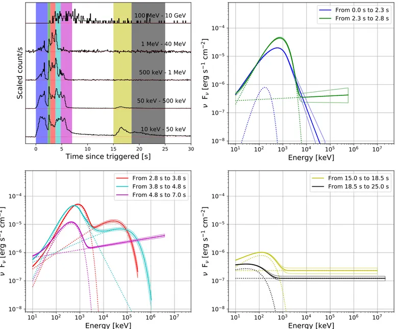
The time interval from T0to T0+ 25 s was subdivided into seven intervals after considering the temporal characteristics shown in Figure 2. Figure 2also shows the best-fit model for each time interval. The spectrum of thefirst pulse phase (T0+ 0–2.3 s) is best fitted with the Band + BB model. The addition of the BB component to the Band component is weakly preferred (ΔBIC∼2). The peak energy (Epk) for the Band component is 586±14 keV, and the temperature of the BB component is 44±5 keV. The temperature of the BB component is consistent with similar components seen in other bright GRBs(Guiriec et al.2011,2013; Axelsson et al.2012).
The main spectral component during the brightest emission episode observed from T0+ 2.3 s to T0+ 7.0 s is characterized by many short and overlapping pulses and is bestfit by either a CPL or Band function. During this phase, the low-energy spectral index is very hard, ranging between−0.4 and 0.0 (see Table1). The peak energy (Epk) reaches a maximum value of Epk∼815 keV from T0 + 2.8 s to T0 + 3.8 s, before decreasing in time(see Table1).
An additional PL or CPL component begins to appear during the T0+ 2.3 s to T0+ 2.8 s time interval and lasts throughout the prompt emission phase. Arrival of the first LAT events above 100 MeV associated with the source begins at T0 + ∼2.7 s, consistent with the emergence of this spectral component. In the third(T0+ 2.8 s to T0+ 3.8 s) and fourth (T0 + 3.8 s to T0 + 4.8 s) time intervals, this additional component increases in brightness and exhibits a high-energy cutoff which increases in energy with time, ranging from 26–52 MeV (see Table 1). The high-energy cutoff is strongly
required in both time intervals compared to the models without
the high-energy cutoff(ΔBIC?10). After ∼4.8 s, the high-energy cutoff in this additional component disappears, and the high-energy emission is well described by a PL with a photon index (dN dEµEGph) of Gph,PL= -1.860.01 or corre-spondingly an energy index(Fnµnb) of b = -PL 0.860.01. After the bright emission phase, the long-lived extended emission observed by the LAT is best described by a PL with an almost-constant photon index of Gph,PL~ -2, as shown in Figure 3. Figure 3 also shows that the energy flux of this extended emission phase (100 MeV–1 GeV) shows a power-law decay in time ( µFn ta), with an exponent of aLAT= -1.090.02. Extrapolation of this extended emission back into the earlier bright emission phase reveals that theflux from the additional spectral component in the prompt emission evolves similarly to the extended emission. This implies that the emission from the additional component and the extended emission may be from the same region. Because the power-law spectral and temporal characteristics of this broadband emission resemble the representative features of GRB after-glows, the end of the bright emission phase at about ∼7 s represents the transition from the prompt to afterglow-dominated emission.
In addition to the extended emission, a weaker, short-duration pulse, with soft emission primarily below100 keV, is observed from T0+ 15 s to T0+ 25 s. This weak pulse, along with the long-lasting extended emission, is well described by the CPL + PL model. For these periods, we fix the photon index of the PL component to−2.0, assuming that the photon index of the energy spectrum of the extended emission is unchanged in time.
4.2.2. Fermi–Swift Joint Spectral Analysis
We continue the time-resolved spectral analysis from T0+ 68.27 s to T0+ 627.14 s, but now include Swift data. For GBM, we prepared the data using the same process as described in Section 4.2.1, although for this time interval we excluded channels below 50 keV because of apparent attenuation due to partial blockage of the source by the spacecraft that is not accounted for in the GBM response. For LAT, we decreased the ROI radius to 10° and increased the maximum zenith angle cut to 110°. Both changes are made in order to reduce the loss of exposure that occurs when the ROI crosses the zenith angle cut and begins to overlap Earthʼs limb. This increase in exposure, though, comes at the expense of increased back-ground during intervals when Earthʼs limb is approaching the burst position. The rest of the process is the same as described in Section4.2.1.
We retrieve Swift data from the HEASARC archive. The BAT spectra are generated using the event-by-event data collected from T0,BAT-239 s to T0,BAT+963 s, with the standard BAT software (HEASOFT 6.2592) and the latest calibration database (CALDB93). The burst left the BAT FoV at ~T0,BAT+720 s and was not reobserved until ~T0,BAT+3800 s. For the intervals that include spacecraft slews, an average response file is generated by summing several short-interval (5 s) response files, weighted by the counts in each interval(see Lien et al.2016, for a more detailed description).
89
http://fermi.gsfc.nasa.gov/ssc/
90http://fermi.gsfc.nasa.gov/ssc/data/access/lat/BackgroundModels.html 91
The difference between the P8R2 and P8R3 isotropic spectra are small and do not affect the results of this analysis.
92http://heasarc.nasa.gov/lheasoft/ 93
http://heasarc.gsfc.nasa.gov/docs/heasarc/caldb/swift/ 7
The XRT acquired the source at T0 + 64.63 s and started taking WT data at T0+ 68.27 s. In the analysis that follows, the XRT data were initially processed by the XRT data analysis software tools available in HEASOFT version 6.25, using the gain calibration files released on 2018 July 10. Prior to extracting spectra, we processed the WT event data using an updated, but as yet unreleased, version of the XRT science data analysis task XRTWTCORR (version 0.2.4), which includes a
new algorithm for identifying unwanted events caused by the delayed emission of charge from deep charge traps that have accumulated in the CCD due to radiation damage from the harsh environment of space. Such trailing charge appears as additional low-energy events and can cause significant spectral distortion at low energies, especially for a relatively absorbed extragalactic X-ray source, like GRB 190114C. Once identi-fied, the trailing charge events were removed from the event list, resulting in clean WT spectra that are usable below 0.7 keV. The XRT spectral extraction then proceeded using standard Swift analysis software included in HEASOFT
software(version 6.25). Grade 0 events were selected to help mitigate pileup and appropriately sized annular extraction regions were used, when necessary, to exclude pileup from the core of the WT point-spread function (PSF) profile when the source count rate was greater than ∼100 cts s−1. PSF and exposure-corrected ancillary response files were created to ensure correct recovery of the source flux during spectral fitting.
We tested three models in the joint spectral fits, a PL, a broken power law(BKNPL), and a smoothly broken power law (SBKNPL). Each model was multiplied by two photoelectric absorption models, one for Galactic absorption(“TBabs”) and another for the intrinsic host absorption (“zTBabs”). For the Galactic photoelectric absorption model, an equivalent hydro-gen column density is fixed to 7.54×10¹⁹ atoms cm−2 (Willingale et al. 2013). We let the equivalent hydrogen
column density for the intrinsic host absorption model be a free parameter in thefit, but fixed the redshift to z=0.42. Figure 2.The scaled light curves and theνFnmodel spectra(and±1σ error contours) for each of the time intervals described in Section4.2.1. Each SED extends up to the energy of the highest-energy photon detected by LAT. The color-coding used in the shading of time intervals in the top-left panel is carried over to the energy spectra in the other three panels. The dotted lines represent the components of the model spectra. The best-fit model and its parameters are listed in Table1.
Table 1
Spectral Fitting to GBM+ LLE + LAT data (10 keV–100 GeV) for Various Time Intervals
Main component Additional component
From To Modela Norm.b G
ph,low Gph,high Epk Norm.b Gph,PL Epk kT PGstat dof BIC
(s) (s) (keV) (MeV) (keV)
0.0 2.3 Band 0.518-+0.0050.005 −0.73-+0.010.01 −4.00-+0.420.27 548.6-+7.67.7 518/353 542 Band+BB 0.481-+0.0110.011 −0.77-+0.010.01 −4.20-+0.460.31 585.4-+13.614.2 11.54-+4.305.46 44.2-+4.74.9 505/351 540 2.3 2.8 CPL+PL 0.555-+0.0090.009 −0.36-+0.030.03 730.0+-15.516.2 0.018-+0.0040.003 −1.96-+0.060.05 425/352 454 2.8 3.8 CPL+PL 0.374-+0.0060.006 −0.09-+0.030.03 840.8-+12.913.1 0.040-+0.0020.002 −1.68-+0.010.01 769/352 799 CPL+CPL 0.355-+0.0070.007 −0.04-+0.030.03 814.9-+13.013.4 0.061-+0.0040.004 −1.43-+0.020.02 26.1-+2.32.6 477/351 512 3.8 4.8 Band+PL 0.706-+0.0110.011 -0.05-+0.030.03 −3.60-+0.190.28 562.8-+9.29.6 0.050-+0.0030.003 −1.64-+0.020.02 577/351 612 Band+CPL 0.675-+0.0100.010 −0.05-+0.030.03 −3.63-+0.260.21 563.1-+9.68.8 0.065-+0.0040.004 −1.64-+0.020.02 51.5-+7.49.8 519/350 560 4.8 7.0 CPL+PL 0.322-+0.0060.006 −0.30-+0.040.04 425.4-+7.47.7 0.057-+0.0020.002 −1.86-+0.010.01 467/352 494 15 18.5 CPL+PL 0.080-+0.0050.005 −1.41-+0.060.08 122.9-+6.77.5 0.014-+0.0030.003 −2.00fixed 407/353 430 18.5 25 CPL+PL 0.030-+0.0040.005 −1.74-+0.080.09 27.7-+4.13.3 0.008-+0.0010.001 −2.00fixed 454/353 478
Notes.Errors correspond to a 1σ confidence region.
a
For the PL, CPL, and Band models, the pivot energy isfixed to 100 keV.
b Photons cm−2s−1keV−1. 9 The Astrophysical Journal, 890:9 (19pp ), 2020 February 10 Ajello et al.
We divided the extended emission phase, T0+ 68.27 s to T0 + 627.14 s, into four time intervals covering 68.27–110 s, 110–180 s, 180–380 s, and 380–627.18 s. The fit results for all four time intervals are listed in Table2. For thefirst two time
intervals, we fit the XRT, BAT, GBM, and LAT data
simultaneously by using different fit statistics for each data type: Cstat (Poisson data with Poisson background) for the XRT, χ2 for the BAT data, and PGstat for GBM and LAT. These statistics are reported independently for each data set in Table2. As shown in Table2and Figure4, a BKNPL function is statistically preferred over the PL and SBKNPL functions in both time intervals, where Figure 4 also includes the spectral fitting results using each individual instrument. When the smoothness parameter s in the SBKNPL model is left free to vary, a sharp break with s>10 is obtained, at which point an SBKNPL resembles a traditional BKNPL model. The low- and high-energy photon indices in the BKNPL model are consistent
in both time intervals, yielding Gph,low~ -1.6 and Gph,high~ -2.1, respectively, with break energies of 4.22-+0.67
0.31 keV and
-+
5.11 0.370.42 keV. We note that the high-energy photon index is consistent with the values in the additional component seen in the prompt phase. This result implies that BAT, GBM, and LAT are observing emission from the same side of the break in the energy spectrum from 10 keV to 100 GeV, which starts to appear during the prompt emission phase in the form of an additional spectral component, whereas the low-energy chan-nels of the XRT are measuring the energy spectrum below this break.
Because the burst is outside the LAT FoV during the last two time intervals, we limit the joint fit during these intervals to XRT and BAT data. We again simultaneouslyfit the data to PL and BKNPL models, using again differentfit statistics for each data type,χ2for the BAT data and Cstatfor the XRT. Again, Figure 3.Temporal and spectral evolution of each spectral component. Top panel: energyflux in the 10 keV–1 MeV (blue) and 100 MeV–1 GeV (green) energy ranges. Middle panel: photon index(for the Band function, we refer to the low-energy photon index). Bottom panel: Epk, where we use the trigger time T0
the BKNPL model is statistically preferred over the simpler PL model. For the time interval from T0+ 180 s to 380 s, the low-and high-energy photon indices, as well as the break energy, in the BKNPL model are consistent with those found during the earlier intervals. For the last time interval from T0+ 380 s to 627.14 s, the low-energy photon index is slightly softer than previous intervals, with Gph,low= -1.710.05, and the break energy is almost consistent with previous intervals.
4.3. Multiwavelength Afterglow Light Curves
Figure5 shows light curves of GRB 190114C for the XRT, BAT, GBM, and LAT data. The selection for the GBM and LAT data is described in Section4.2.1, and theflux is calculated from the best-fit function for each time interval in the spectral analysis with each individual instrument. The XRT (0.7 keV–10 keV), and BAT (15 keV–50 keV) light curves are obtained from the UK Swift Science Data Centre. The UVOT(2–5 eV for the white band) light curve is obtained by uvotproduct of the HEASoft package. The BAT, GBM, and LAT light curves show an obvious transition from the highly variable prompt emission to a smoothly decaying afterglow component (αBAT=−1.00± 0.01, αGBM=−1.10±0.01, and αLAT=−1.22±0.11). At later times, all three light curves decay in time with consistent decay indices, α∼−1, implying that they originate from the same emitting region.
The XRT light curve is well described by a broken power law with temporal indicesαXRTof−1.30±0.01 and −1.49± 0.02 with the break occurring at approximately tbreak∼T0+ ∼19.8×10³s(∼5.5 hr) (see inset in Figure5). The prebreak decay index of the XRT light curve differs from the indices measured for the BAT, GBM and LAT data. This difference in
decay slopes indicates that the XRT is probing a different portion of the afterglow spectrum, a conclusion that is consistent with the observed spectral breaks in the Swift and Fermi joint-fit spectral analysis (Section4.2.2).
On the other hand, the UVOT light curve exhibits decay slopes and a temporal break that are distinct from the XRT and BAT data. The temporal break occurs at∼400 s, with temporal indicesαUVOTbefore and after the break of−1.62±0.04 and −0.84±0.02, respectively. These decay indices are steeper than the decay observed in the XRT before the break in the UVOT data and shallower than the XRT decay afterwards. This implies that the UVOT is observing yet another distinct portion of the afterglow spectrum. These observations can be interpreted as the contribution of an optically bright reverse shock that becomes subdominant to the forward-shock emission at the time of the observed temporal break. In such a scenario, the postbreak decay index seen in the UVOT would then reflect a distinct portion of the afterglow spectrum below the X-ray regime.
5. Discussion 5.1. Prompt Emission
The prompt emission observed in GRB 190114C resembles the complex relationship between multiple emission compo-nents commonly seen in LAT-detected GRBs. The emission observed in the first ∼2 s is best characterized as a Band function spectrum with a possible subdominant BB component, which combined produce no detectable emission in the LAT energy range. The energyfluxes of the thermal and nonthermal components in the energy band from 10 keV to 1 MeV are Table 2
Spectral Fitting to Fermi and Swift data(1 keV–100 GeV) for Various Time Intervals
From To Modela,b Gph,low Gph,high Ebreak p N(H) PGstat Cstat c2 dof BIC
(s) (s) (keV) (1022 atoms cm−2) 68.27 110 PL −2.09-+0.010.01 10.55+-0.260.27 504 655 52 1086 1239 BKNPL −1.55-+0.120.12 −2.11-+0.020.02 4.72-+0.371.20 8.22-+0.520.54 502 625 56 1084 1225 SBKNPLISMc −(p+1)/2 −(p+2)/2 4.63-+3.283.38 2.46+-0.110.08 9.91-+0.260.27 504 642 55 1085 1236 SBKNPLwindd −(p+1)/2 −(p+2)/2 7.46-+6.6372.89 2.54+-0.160.15 10.06-+0.260.27 504 644 54 1085 1238 110 180 PL −2.00-+0.020.02 10.42+-0.230.23 616 671 50 1087 1364 BKNPL −1.57-+0.080.08 −2.06-+0.020.02 5.60-+0.460.76 8.30-+0.390.40 616 627 51 1085 1336 SBKNPLISM −(p+1)/2 −(p+2)/2 2.56-+1.544.20 2.24-+0.080.10 9.74-+0.230.23 621 653 50 1087 1358 SBKNPLwind −(p+1)/2 −(p+2)/2 1.69-+0.694.63 2.26-+0.100.10 9.89-+0.230.23 621 656 50 1086 1362 180 380 PL −1.90-+0.010.01 9.57-+0.150.17 774 66 810 866 BKNPL −1.54-+0.060.06 −1.99-+0.050.05 5.18-+0.360.46 7.93-+0.280.29 727 63 808 830 SBKNPLISM −(p+1)/2 −(p+2)/2 5.60-+1.5120.145 2.20-+0.020.10 9.07-+0.140.15 756 64 809 854 SBKNPLwind −(p+1)/2 −(p+2)/2 6.88-+0.440.35 2.25-+0.020.16 9.21-+0.150.16 761 64 809 858 380 627.14 PL −1.86-+0.010.01 9.09-+0.140.13 700 47 839 775 BKNPL −1.71-+0.050.05 −2.11-+0.090.08 5.52-+0.380.72 8.43-+0.230.24 686 42 837 768 SBKNPLISM −(p+1)/2 −(p+2)/2 8.67-+6.7837.30 2.18-+0.160.20 8.67-+0.110.20 694 44 838 772 SBKNPLwind −(p+1)/2 −(p+2)/2 9.16-+4.9136.96 2.20-+0.100.19 8.77-+0.090.18 695 45 838 774
Notes.Errors correspond to the 1σ confidence region.
a
Because the XRT data are included, a model is multiplied by the photoelectric absorption models, TBabs withfixed hydrogen column density of 7.54×1019cm−2 and zTBabs withfixed redshift of 0.4245.
b
Note that a“constant” factor is included in the model, which accounts for the potential of relative calibration uncertainties in the recovered flux (i.e., normalization) between BAT and GBM. The factor ranges from 0.8 to 1.3, which is acceptable.
cSmoothness parameter s=1.15–0.06p (Granot et al. 2002). dSmoothness parameter s=0.80–0.03p (Granot et al.
2002).
11
∼1.1×10⁻⁶and∼3.9×10⁻⁵erg cm−2s−1, respectively. We estimate the ratio of the thermal to nonthermal emission during this period to be approximately 3%.
The delay in the onset of the LAT-detected emission is related to the emergence of a hard PL component superimposed on the highly variable Band+BB component seen in the GBM. Furthermore, the PL component is initially attenuated at energies greater than∼100 MeV, and we interpret this spectral turnover as due to opacity to electron–positron pair production (gg e e+ -) within the source. The cutoff energy associated with this turnover is observed to increase with time before disappearing entirely at later times. Similar behavior has been observed in other LAT-detected bursts (e.g., GRB 090926A; Ackermann et al. 2011) and has been attributed to the
expansion of the emitting region, as the pair production opacity is expected to scale as tggµR-1for afixed mean flux, where R is the distance from the central engine.
As has also been noted for other LAT-detected GRBs, e.g., GRBs 081024B(Abdo et al.2010), 090510 (Ackermann et al. 2010), 090902B (Abdo et al. 2009a), 090926A (Ackermann
et al.2011), 110731A (Ackermann et al.2013b), and 141207A
(Arimoto et al.2016), the existence of the extra PL component
can be seen as a low-energy excess in the GBM data. This
observation disfavors SSC or IC emission from the prompt emission as the origin of the extra PL component, as SSC emission cannot produce a broad power-law spectrum that extends below the synchrotron spectral peak. Instead, we identify this component as the emergence of the early afterglow over which the rest of the prompt emission is superimposed. Similar conclusions have been drawn by Ravasio et al.(2019)
as to the origin of the PL component seen in the GBM data.
5.2. Afterglow Emission
The Swift and Fermi data reveal that the power-law spectral component observed during the prompt emission transitions to a canonical afterglow component, which fades smoothly as a power law in time. In the standard forward-shock model of GRB afterglows (Sari et al. 1998), specific relationships
between the temporal decay and spectral indices, the so-called “closure relations,” can be used to constrain the physical properties of the forward shock as well as the type of environment in which the blast wave is propagating.
Our broadband fits to the simultaneous XRT, GBM, BAT, and LAT data show evidence for a spectral break in the hard X-ray band (5–10 keV). In the context of the forward-shock model, this spectral break could represent either the frequency Figure 4.Spectral energy distributions from optical to gamma-ray energies for the four time intervals(T0+ 68.27 s to 110 s, T0+ 110 s to 180 s, T0+ 180 s to 380 s, and T0+ 380 s to 627 s) described in Section4.2.2. The solid black lines represent the best-fitting broken power-law function. Each filled region corresponds to the 1σ error contour of the best-fit law function to the data from each individual instrument. The cyan regions are an extrapolation from the best-fitting broken power-law function. The dotted line denotes the best-fit break energy Ebreak. The simultaneous UVOT white- and u-band observations taken during the T0+ 180 s to 380 s and T0+ 380 s to 627 s intervals are also shown but are not included in the joint spectral fit. Note that the UVOT observations are uncorrected for Galactic or host absorption and as such serve as lower limits to the UV and opticalflux.
of the synchrotron emission electrons with a minimum Lorentz factorνmor the cooling frequency of the synchrotron emission νc. Because there are no additional spectral breaks observed up to and through the LAT energy range, if we assume the observed spectral break is either νm or νc, then we naturally hypothesize thatνc<νmorνm<νc, respectively. In the case where the spectral break isνm, the low-energy and high-energy photon indices are expected to be ν−1.5 for ν<νm and n- +(p 2) 2~n-2.1 for ν>νm, when assuming an electron spectral index of p ∼ 2.1, a characteristic value obtained in previous studies (e.g., Waxman 1997; Bednarz & Ostrowski
1998; Freedman & Waxman2001; Curran et al. 2010; Wang et al. 2015). These values are consistent with the observed
photon indices, although the expected temporal index when ν<νmis expected to be∝t−1/4, which is inconsistent with the XRT decay index of∝t−1.32±0.01for either a constant-density (ISM) or wind-like (wind) circumstellar environment. There-fore, this scenario in which the break is due toνmis disfavored. In the case where the spectral break isνc, the low-energy and high-energy photon indices are expected to be n- +(p 1) 2~ n-1.6 for ν<νc and n- +(p 2) 2~n-2.1 for ν>νc, again assuming p∼2.1, again consistent with the observed values. The expected temporal behavior whenν>νcin both the ISM and wind cases is µt(2 3-p) 4~t-1.1, which is consistent with the temporal decay measured in the BAT, GBM, and LAT energy ranges. For ν<νc, the expected temporal behavior significantly depends on the density profile of the circumstellar environment. In the ISM case, the temporal index is expected to be µt3 1( -p) 4~t-0.8, inconsistent with the decay observed
in the XRT, whereas for the wind case, the expected temporal index is µt(1 3- p) 4~t-1.3, matching the decay seen in X-rays. If we are indeed observing an afterglow spectrum in which the XRT data are belowνc, then we can follow the formalism established in Sari & Mészáros(2000) and van Eerten & Wijers
(2009) to estimate an arbitrary circumstellar density profile
index k, for n r( )µR-k, to be k=(12β–8α)/(1 + 3β– 2α)=1.92±0.07, which also supports a wind profile (k=2) scenario.
Figure6shows the observed evolution of Ebreakin the four time intervals we analyzed, along with the expected evolution of the cooling break n µc t+1 2in a wind-like environment. Despite an initial increase in the break energy between thefirst two intervals, the break energy is consistent with remaining constant after T0>150 s. This behavior is similar to that observed for GRB 130427A, in which the broadband modeling preferred a wind-like environment(Perley et al.2014), but for which νcwas nonetheless observed to remain constant through the late-time observations (Kouveliotou et al. 2013). Kouveliotou et al. (2013) concluded
that GRB 130427A may have occurred in an intermediate environment, possibly produced through a stellar eruption late in the life of the progenitor which altered the circumstellar density profile (Fryer et al.2006). Nonetheless, a wind-like environment
for GRB 190114C matches conclusions drawn by Cenko et al. (2011), Ackermann et al. (2013b), and Ajello et al. (2018) from
a growing number of bursts for a possible preference for LAT-detected bursts to occur in stratified environments, despite the observation that the majority of long GRB afterglows are Figure 5.Multiwavelength afterglow light curves for the UVOT(yellow), XRT (red), BAT (blue), GBM (green), and LAT (purple) data from GRB 190114C. The flux for the GBM (10 keV–1 MeV) and LAT (100 MeV–1 GeV) data is calculated from the best-fit model for each time interval in the spectral analysis with each instrument. The BAT, GBM, and LAT emission show a transition after∼T0+ 10 s to an extended emission component decaying smoothly as a power law in time (solid lines). Both the XRT and the UVOT light curves are well described by a broken power law, respectively (solid lines), and their break times are 19.8×10³
s (∼5.5 hr) and 377 s, respectively (dotted lines). The inset shows the light curves of the LAT, XRT, and UVOT up to ∼T0+ 23 days.
13
otherwise consistent with occurring in environments that exhibit uniform density profiles (Schulze et al.2011).
The temporal decay of the UVOT data, although uncorrected for either Galactic or host-galaxy extinction, can provide additional constraints on the location of νm. The UVOT emission decays as a broken power-law function, starting with
-
t 1.62 0.06 from 70 to 400 s, before transitioning to a slower decay oft-0.84 0.03 for 400–105
s. The prebreak emission can be interpreted as the contribution from a reverse shock, which is expected to exhibit a temporal index of µt-(73p+21) 96~
-t 1.82, assuming p=2.1 (Kobayashi2000), roughly consistent with observations. If the UVOT-observed emission after T0+ ∼400 s is due to the forward-shock component in which the UVOT data are aboveνmbut belowνc, then the temporal decay is expected to be µt(1 3- p) 4~t-1.3 for p=2.1, which is too steep with respect to the observed postbreak UVOT decay (t-0.84 0.03 ). On the other hand, if the UVOT data are below both νmandνc, the temporal decay is expected to beflat, ∝t0. Without a clear preference for either of the two scenarios, we conjecture that the UVOT-detected emission may have a different origin or emission site than the X-ray and gamma-ray emission.94
5.3. Energetics
GRB 190114C was exceptionally bright in the observer frame. The one-second peak photon flux measured by GBM is 247±1 photons s−1cm−2, with a total fluence of (4.433±0.005)×10−4erg cm−2, both in the 10–1000 keV band. This makes GRB 190114C the fourth brightest in peak flux and the fifth most fluent GRB detected by GBM, placing it in the top 0.3 percentile of GRBs in the third GBM catalog (Bhat et al.2016).
Thefluence in the 100 MeV–100 GeV energy band measured by the LAT, including the prompt and extended emission, is (2.4±0.4)×10−5erg cm−2, which sets GRB 190114C as the second mostfluent GRB detected by the LAT. Figure7 shows the 10–1000 keV fluence versus the 0.1–100 GeV fluence for GRB 190114C in comparison with the sample of GRBs detected by the LAT from the 2FLGC. Thefluence measured by the LAT is only slightly smaller than that of GRB 130427A, currently the mostfluent GRB detected by the LAT.
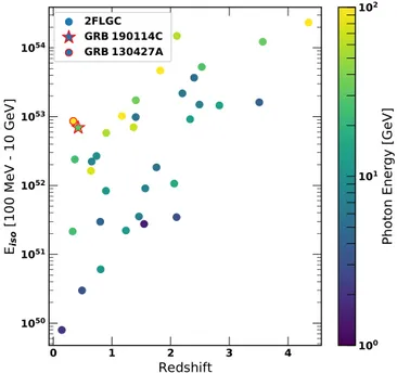
At a redshift of z=0.42 (dL=2390 Mpc), the total isotropic-equivalent energies Eisoreleased in the rest-frame GBM(1 keV– 10 MeV), LAT (100 MeV–10 GeV), and combined (1 keV– 10 GeV) energy ranges are (2.5±0.1)× 1053erg,(6.9±0.7)× 1052 erg, and (3.5±0.1)×1053 erg, respectively. We also estimate a one-second isotropic-equivalent luminosity of Lγ,iso= (1.07±0.01)×1053erg s−1in the 1–10,000 keV energy range. Figure8shows Eisoestimated in the 100 MeV–10 GeV rest frame along with the sample of the 34 LAT-detected GRBs with known redshift in the 2FLGC. We note that GRB 190114C is among the most luminous LAT-detected GRBs below z<1, with an Eiso just below GRB 130427A, which also exhibited the highest-energy photons detected by the LAT from a GRB, including a 95 GeV photon emitted at 128 GeV in the rest frame of the burst.
5.4. Bulk Lorentz Factor
GRBs are intense sources of gamma-rays. If the emission originated in a nonrelativistic source, it would render gamma-ray photons with energies at the nF peak energy and aboven susceptible to e±-pair production(gg e) due to high optical depths(t Ggg( bulk,E) 1) for γγ-annihilation. This is the so-called “compactness problem,” which can be resolved if the emission region is moving ultrarelativistically, with Γbulk 100, toward the observer(Baring & Harding1997; Lithwick & Sari2001; Granot et al.2008; Hascoët et al.2012). In this case,
the attenuation offlux, which either appears as an exponential Figure 6.Observed spectral break energy vs. time. The blue and green points
represent the break energy(Ebreak) in the BKNPL and SBKNPLwindmodels in
the four time intervals, respectively. The dashed line represents the cooling frequency with time (n µc t+1 2) expected from the afterglow parameters.
Despite an initial increase in the break energy between thefirst two intervals,
the break energy is consistent with remaining constant after T0+ ∼150 s. Figure 7.Fluence in the energy range of 0.1–100 GeV vs. 10 keV–1 MeV for
GRB 190114C(star) compared with the sample of 186 LAT-detected GRBs from the 2FLGC. Red points are for short GRBs while blue points are for long GRBs.
94
Although Laskar et al.(2019) suggested that the system is in fast cooling to explain the temporal and spectral behaviors in the optical and XRT bands, the fast-cooling scenario may face difficulty in reproducing different temporal behaviors between the XRT and BAT bands (i.e., αXRT∼−1.3 and αBAT∼−1.0).
cutoff or a smoothly broken power law (Granot et al.2008, hereafter G08), due to γγ-annihilation occurs at much higher
photon energies above the peak of the νFν spectrum where t Ggg( bulk,E>Ecut)>1. Such spectral cutoffs have now been observed in several GRBs, e.g., GRB 090926A (Ackermann et al. 2011), and GRBs 100724B and 160509A (Vianello et al. 2018); also see Tang et al. (2015) for additional sources. Under
the assumption that these cutoffs indeed result from γγ-annihilation, they have been used to obtain a direct estimate of the bulk Lorentz factor of the emission region. When no spectral cutoff is observed, the highest-energy observed photon is often used to obtain a lower limit on Γbulkinstead. In many cases, a simple one-zone estimate ofτγγwas employed, which makes the assumption that both the test photon, with energy E, and the annihilating photon, with energy Gbulk m ce E 1+z
2 ( 2 2) ( ) ,2 were produced in the same region of theflow (e.g., Lithwick & Sari 2001; Abdo et al.2009b). Such models yield estimates of
Γbulkthat are typically larger by a factor∼2 than that obtained from more detailed models ofτγγ. The latter either feature two distinct emission regions(a two-zone model; Zou et al.2011) or
account for the spatial, directional, and temporal dependence of the interacting photons(G08; Hascoët et al.2012). Here we use
the analytic model of G08, which assumes an expanding ultrarelativistic spherical thin shell and calculatesτγγ along the trajectory of each test photon that reaches the observer. The results of this model have been independently confirmed with numerical simulations(Gill & Granot2018), which show that it
yields an accurate estimate ofΓbulkfrom observations of spectral cutoffs if the emission region remains optically thin to Thomson scattering due to the produced e±pairs. In this case, the initial bulk Lorentz factor of the outflow Gbulk,0 is estimated using
G = + ´ -G G -+G - - G 1 C z L E t 100 396.9 1 10 erg s 5.11 GeV 2 33.4 ms . v bulk,0 2 0 52 1 cut 1 ph 5 3 1 2 2 ph ph ph ( ) ( ) ( ) ⎡ ⎣ ⎢ ⎛ ⎝ ⎜ ⎞⎠⎟ ⎛ ⎝ ⎜ ⎞ ⎠ ⎟ ⎛⎝⎜ ⎞⎠⎟ ⎤ ⎦ ⎥ ⎥
Here, tvis the variability timescale,Γphis the photon index of the PL component, andL0=4pdL2(1 +z)-G -ph 2F0, where dLis the luminosity distance of the burst, F0 is the (unabsorbed) energyflux (νFν) obtained at 511 keV from the PL component of the spectrum. The parameter C2≈1 is constrained from observations of spectral cutoffs in other GRBs(Vianello et al.
2018). The estimate of the bulk Lorentz factor in Equation (1)
should be compared with Gbulk,max=(1+ z E) cut m ce 2, which corresponds to the maximum bulk Lorentz factor for a given observed cutoff energy and for which the cutoff energy in the comoving frame is at the self-annihilation threshold,
¢ = + G =
Ecut (1 z E) cut bulk m ce 2 (however, see, e.g., Gill & Granot 2018, where it was shown that the comoving cutoff energy can be lower than mec2due to Compton scattering by e± pairs). The true bulk Lorentz factor is then the minimum of the two estimates.
In GRB 190114C, the additional PL component detected by the LAT exhibits a significant spectral cutoff at Ecut∼ 140 MeV (where Ecut=Epk/(2+Γph)) in the time period from T0+ 3.8 s to T0+ 4.8 s. Using the variability timescale in the GBM band of tv∼6 ms, where we assume that the GBM and LAT emissions are cospatial, we obtain the bulk Lorentz factor Gbulk,0~ 210 from Equation (1), which is lower than Gbulk,max» 400 and is therefore adopted as the initial bulk Lorentz factor of the outflow.
5.5. Forward-shock Parameters
The timescale on which the forward shock sweeps up enough material to begin to decelerate and convert its internal energy into observable radiation depends on the density of the material into which it is propagating A, the total kinetic energy of the outflow (Eiso/η∼1.8×1054 erg, where Eiso=3.5× 1053erg∼1053.5erg and η=0.2 is the conversion efficiency of total shock energy into the observed gamma-ray emission), and its initial bulk Lorentz factor Gbulk,0. Here, in a wind environment, we define a timescale tγ on which the accumulated wind mass is 1/Gbulk,0 of the ejecta mass as
p h h = + G ~ ´ G g -- - t E z Am c A E 1 16 2 s 10 ergs 0.2 200 , 2 p iso 3 bulk,0 4 1 iso 53.5 1 bulk,0 4 ( ) ( ) ⎜ ⎟ ⎜ ⎟ ⎛ ⎝ ⎜ ⎞ ⎠ ⎟⎛⎝ ⎞⎠ ⎛⎝ ⎞⎠
where A=3´1035Acm-1 with a mass-loss rate 10−5 M☉ yr−1in the wind velocity of 103km s−1for Aå=1. If the reverse shock is Newtonian, or at least mildly relativistic(i.e., the thin-shell limit; Sari & Piran1995; Zhang et al.2003), tγis the deceleration time tdec. In the thin-shell case, to obtain the observed temporal onset at T0+ ∼10 s, Aå=0.2 is needed. If the reverse shock is relativistic(thick-shell limit), one has tdec∼tGRB>tγ(tGRBis the burst duration), which approximately gives Aå>0.2.
Having constrained the location of the synchrotron break energies and the likely environment into which the blast wave is propagating, we can invert the equations governing the energies of these breaks to estimate the physical properties of the forward shock. These include the microphysical parameters describing the partition of energy within the shock, the total energy of the shock EK(=Eiso/η), and the circumstellar density normalization Aå. The equations governing the location of nm, Figure 8.Scatter plot of Eiso(100 MeV–10 GeV) vs. redshift for various GRBs
including GRB 190114C (star). Colors indicate the energy of the highest-energy photon for each GRB with an association probability>90%.
15