A Zoomable 3D User Interface using Uniform Grids and Scene Graphs

(1)

A Zoomable 3D User Interface using Uniform Grids and Scene

Graphs

Master Thesis in Computer Science

Vidar Rinne

School of Innovation, Design and Engineering

M¨

alardalen University

V¨

aster˚

as, Sweden

November 25, 2011

Supervisor:

Thomas Larsson

School of Innovation, Design and Engineering M¨alardalen University

(2)

Abstract

Zoomable user interfaces (ZUIs) have been studied for a long time and many applications are built upon them. Most applications, however, only use two dimensions to express the content. This report presents a solution using all three dimensions where the base features are built as a framework with uniform grids and scene graphs as primary data structures. The purpose of these data structures is to improve performance while maintaining flexibility when creating and handling three-dimensional objects. A 3D-ZUI is able to represent the view of the world and its objects in a more lifelike manner. It is possible to interact with the objects much in the same way as in real world. By developing a prototype framework as well as some example applications, the usefulness of 3D-ZUIs is illustrated. Since the framework relies on abstraction and object-oriented principles it is easy to maintain and extend it as needed. The currently implemented data structures are well motivated for a large scale 3D-ZUI in terms of accelerated collision detection and picking and they also provide a flexible base when developing applications. It is possible to further improve performance of the framework, for example by supporting different types of culling and levels of detail.

(3)

1 Introduction

Zoomable User Interfaces (ZUIs) also called Multi-scale Interfaces are very common and many devel-opers are building systems based on them [12]. A ZUI is designed so that users can see an overview of the content in the application which is achieved by the ability to zoom [18]. The zoom effect can be made in different ways, for example zooming a spe-cific object or zooming the entire view [12]. Objects can also be replaced with different level of details at different zoom levels [12]. Many ZUIs are made using two dimensions such as ZoneZoom and Pho-toMesa [5, 7, 20] but there are a few known three-dimensional zoomable user interfaces such as Bum-Top [1] and Google Earth [9]. Zoomable interfaces can hold and view many objects at the same time which makes performance a problem, for example rendering speed when many objects are visible but also collision detection between objects. Another known problem with ZUIs is that users can get dis-oriented when navigating and not knowing how to use the interface to get back to the recent state, Stu-art Pook et al. are describing these users as “lost in hyperspace” [18, p1]. Other evaluations [1, 5, 7, 17] report that users liked the interfaces in different ways.

The purpose of this project is to explore how 3D-ZUIs can be built, how flexible they can be and what they can be used for. The base features of a ZUI were implemented into a framework on which several example applications were built. The frame-work was developed to support the basic functions and features needed for the example applications including the two major data structures used in this project which are the uniform grid and the scene graph, both are explained in the following sec-tions. The example applications are a photo viewer demonstrating features like zooming, throwing and collision detection using a uniform grid, a scene viewer demonstrating the strengths of the scene graphs, a floating control example with event han-dling and node search and at last a multitexturing example, all to demonstrate some of the frameworks most important capabilities. The example applica-tions are written in MSVS1 _{C++ using GLEW}2_,

GLUT3 _{and SDL}4 _{as graphics libraries, the three}

libraries are based on OpenGL.

This report is structured as follows: chapter two presents related work on scene graphs, uni-form grids and 2D- and 3D-ZUIs. Chapter three presents the framework and its capabilities includ-ing algorithms and data structures. Chapter four

describes the example applications developed dur-ing this project. Chapter five presents the results including theoretical performance and pilot study. Chapter six presents conclusions and future work. The seventh and final chapter contains a list of all references used in the project.

2 Related Work

A common topic for uniform grids is ray tracing as the purpose of the grid is to divide space and related data into partitions to reduce intersection tests [10, c7, p285]. The grid is used to reduce the ray/object intersection tests for a ray in 2D-or 3D-space. By registering objects into partitions and traversing the grid it is possible to faster deter-mine nearby objects. Common algorithms used for ray traversal in a grid are often based on a Digital Differential Analyzer (DDA) such as “A Fast Voxel Traversal Algorithm for Ray Tracing” presented by John Amanatides and Andrew Woo [3]. It is de-scribed as a simple high performing algorithm that needs only a few comparisons for ray traversal and it also requires little memory.

F. Cazals et al. presents a solution for ray-tracing using uniform grids in the paper “Filtering, Clustering and Hierarchy Construction: a New So-lution for Ray-Tracing Complex Scenes” [11]. The solution of using a hierarchy of uniform grids and filtering and clustering of objects is aimed for more complex scenes. Several structures such as bound-ing volume hierarchies, BSP trees, uniform grids, subdivided uniform grids and octrees are discussed in the paper. During the analysis the author brings up the uniform grid as is having optimal perfor-mance with equally scattered objects but the struc-ture will not handle non-uniform distribution very well. The author claims that experiments are re-quired to find the best trade-off of ”cost of intersec-tions” vs. ”cost of traversal”. A comparisons be-tween recursive grids and hierarchy of uniform grids shows that recursive grid may explode in memory consumption and that it is easier to handle this is-sue in hierarchal uniform grids. In octrees (special case of recursive grid) a voxel is always divided into eight new voxels and the author is describing the tree as unpredictable since it can get very deep and may contain many duplicates.

Uniform grids are also used to optimize perfor-mance in games [25, p249, p385]. Perforperfor-mance de-manding algorithms such as collision detection and picking are accelerated using the grid when there 1_{Microsoft Visual Studio: (www.microsoft.com/visualstudio) Accessed: 23112011}

2_{The OpenGL Extension Wrangler Library: (glew.sourceforge.net) Accessed: 23112011} 3_{The OpenGL Utility Toolkit: (www.opengl.org/resources/libraries/glut) Accessed: 23112011} 4_{Simple DirectMedia Layer: (www.libsdl.org) Accessed: 23112011}

(5)

are many objects in the scene. Picking uses ray traversal to find intersecting objects while collision detection is searching for nearby objects by exam-ining the partitions the object currently is located in. It is also possible to load parts of the map or world at the time depending on an objects location in the grid and to play sound from objects located around a specific location.

A toolkit called IRIS Inventor presented in the paper “IRIS Performer: A High Performance Mul-tiprocessing Toolkit for Real-Time 3D Graphics” written by John Rohlf and James Helman [21] was developed with real-time 3D graphics and perfor-mance in mind. The primary data structure of the toolkit is a hierarchal scene graph which is built of several node types such as scene-, switch-, LOD-, light and group nodes. Some specific pur-poses of the scene graph are that its geometric data structures are optimized for using immediate mode which claims to be a good choice for animations, the scene graph is also constructed to reduce graphics mode changes for faster graphics rendering and also to allow parallel traversal for multiprocessing capa-bilities. Some other speed up techniques are culling, bounding volume hierarchy and level of detail.

Another toolkit presented in the paper “An Object-Oriented 3D Graphics Toolkit ” [23] written by Paul S. Strauss and Rikk Carey is focusing on interactive 3D applications. It is presented as a general, object-oriented and extensible framework aimed for developers. Another goal of this toolkit was to make it interactive and to be able to in-teract directly with 3D-objects which was not very common at the time. The toolkit was built using an object-oriented approach using scene graphs for dy-namic object representation. Some node types are transform-, camera-, light-, material-, and several types of shape nodes. Bounding volumes and event handling were implemented to make the toolkit sup-port picking. Actions like RayPickAction can be used to get the most front object and more informa-tion can be collected by using queries. Picking is ac-celerated by separator nodes which for example can be used to cache bounding boxes for faster culling and real-time highlighting of objects. Another fea-ture that was implemented was the track ball for rotation of objects. It was represented as an inter-active sphere encapsulating 3D-objects. Other per-formance improvements are tuned rendering paths, cached states by storing information in separator nodes and display lists.

The paper “The Data Surface Interaction Paradigm” written by Rikard Lindell and Thomas Larsson [17] presents a solution to make interac-tion easier by developing a prototype live music

tool based on 2D-ZUIs. The application was imple-mented with features like incremental search, zoom, pan and other functions like visual feedback and text completion. The application was evaluated by ten test users and responses were that it felt free and was fun and easy to use [17]. Hierarchical scene graphs were used to represent the components which include information like position and scale. The graphics library used was Simple Direct Me-dia Layer (SDL) based on the OpenGL API along with the FreeType font library that offers texture mapped fonts.

ZoneZoom is a technique for handling input on smart phones. It was developed because of navi-gation difficulties on current smart phones. In the paper written by Daniel C. Robbins et al. [20] they give an example of using their technique on a map navigation software where the keys on the keypad are mapped to nine different grid cells on the map, for example key 4 takes the user to the map cell to the left while 6 to the right, map cell 5 is always in the middle of the screen and allows the user to zoom in on the map part that is currently under the cell. Their conclusion brought up that this system has been adapted to a map monitoring application which has been deployed to over 1000s of users.

Desktop PhotoMesa is a zoomable photo browser which is described in the paper by Ben-jamin B. Bederson and Amir Khella [5, 7]. Pho-toMesa uses tree maps to place pictures on the screen. Pictures in directories are placed in groups. When clicking a specific group the application zooms in on the directory. Low resolution pictures are used as thumbnails but full resolution while zoomed. There are also possibilities to navigate on the screen using the keyboard. The application was implemented in JAVA with the Jazz toolkit [6] which can help building zoomable two-dimensional interfaces using scene graphs. Feedback from users using the pocket version of the PhotoMesa did not notice any increase or reduction in time when com-pared to software that did not have the same fea-tures. Users reported that PhotoMesa was more fun than alternatives and also easy to use.

In George W. Furnas and Xiaolong Zhang’s pa-per [12] they present an application called MuSE (MultiScale Editor). It is written in Td/Tk and Pad++5 _{which is software for creating zoomable}

interfaces. The operating system was UNIX. The purpose of this application was to examine several zooming techniques which are presented in the pa-per, for example bounded-geometric-zooming which means that the object cannot be larger or smaller than specified boundaries. If too large they will become invisible not to cover other objects and If 5_{Pad++ Toolkit: (www.cs.umd.edu/hcil/pad++) Accessed: 23112011}

(6)

too small they can be filtered away. Another sim-ple zoom effect that basically works in the same way is fade-bounded-geometric-zooming which fades the object when it is getting too big or too small on the screen. Fixed-size-zooming gives the effect that the object is fixed but the environment is zoomed. Se-mantic zooming is also discussed which means that objects are replaced while zooming. More zoom-ing effects can be found in George W. Furnas and Xiaolong Zhang’s paper “MuSE: A MultiScale Ed-itor” [12]. Human Computer Interaction Lab is no longer developing or supporting PAD++ but is still exploring ZUIs and is currently working on a new JAVA-based toolkit called Piccolo6_.

The 3D-desktop software called BumTop pre-sented in the paper “Keepin’ It Real: Pushing the Desktop Metaphor with Physics, Piles and the Pen” written by Anand Agarawala and Ravin Balakrish-nan [1] aims at making the desktop more physically correct. It is considered an alternative for regular desktops. The interaction is optimized for using a pen where 3D-icons easily can be moved, thrown as well as selected by lasso tools. Some important de-sign goals presented are smooth transitions and pil-ing. Smooth transitions means that animations are smooth, for example when dragging an object it will increase and decrease in speed instead of clamping to the cursor. Piling means that icons can be on top of each other instead of side by side. It is also pos-sible to browse between the piled objects and to get an overview. The software is using a physics library that takes care of collisions, although physics can be deactivated if necessary. The evaluation shows that users liked the realistic feel, features like throw-ing/tossing and the smooth transitions. Users also reported that they felt familiar with the software and most people completed the training without ex-tensive practicing.

Google Earth is another navigation tool that provides many services [9]. It is using a 3D-globe with satellite images as surface where roads and other choices can be highlighted through settings. Most common places and cities are modeled in 3D. Google Earth also has a street view which makes it possible to navigate as when standing on the street by clicking on cameras in the desired direction. The interface allows the user to grab and drag earth to rotate it in different directions as well as zoom from planetary view to street view. Google Earth also support path finding between selected locations and navigation with GPS.

Microsoft Surface789_{is running on a large touch}

screen table and is intended for multiple people

working on the same project. It is also possible to work from any angle. Microsoft Surface aims at many areas such as IT, education, financial and health care among others. It is a way to connect people, to learn, entertainment and work. Microsoft Surface 2.0 runs on top of Microsoft Windows 7 and has 360 degrees of freedom. It is optimized for over fifty simultaneous touch points and has ob-ject recognition of obob-jects placed on the screen. It is possible to develop custom applications by sup-pressing the Windows 7 interface and use your own touch user interface.

3 The Framework

A framework was developed during this project to support basic 2D/3D-operations and viewing capa-bilities. It is developed with support from a uniform grid which is a partitioning structure and the scene graph for flexible models. The main purpose of the uniform grid is to speed up features like picking and collision detection while the scene graph structure is mainly used for flexible 3D-models. The frame-work is written in C++ using Microsoft Visual Stu-dio and GLEW to get necessary information and at last GLUT and SDL as graphics libraries. The most necessary functions were implemented into the framework to support the features in the example applications. The uniform grid and scene graph and related features got the highest priority.

This section is structured as follows: the first subsection shows some examples of how to use the framework. The second subsection describes the most important algorithms and data structures and the third subsection presents other functionality.

3.1 Using the Framework

There are a few steps necessary to get the features of the framework available. Some example code about how to set up the framework, the scene graph and how to render a scene are described below.

3.1.1 How to Start

To be able to use functions provided by the frame-work the base class must be inherited into a custom class. Below is a piece of code describing the cus-tom class my3DZUI that inherits the properties of the ZUI App class:

class my3DZUI:public ZUI_App{ ...

}; 6_{Piccolo Toolkit: (www.cs.umd.edu/hcil/piccolo) Accessed: 23112011}

7_{Ms Surface Origins: (www.microsoft.com/surface/en/us/Pages/Product/Origins.aspx) Accessed: 23112011} 8_{Developing Applications for Ms Surface: (msdn.microsoft.com/en-us/windows/hh241326.aspx) Accessed: 23112011} 9_{Ms Surface Design & Interaction Guide: (msdn.microsoft.com/en-us/windows/hh241326.aspx) Accessed: 23112011}

(7)

Before the underlying data structures can be used the ZUI App must be initiated. It is achieved by calling the init function which takes the x - and y-resolution and a Boolean value whether the ap-plication should be set to full screen or not. If the window caption is to be set it must be called after the init function.

ZUI_Init(1920, 1080, true);

ZUI_SetCaption("Zoomable User Interface"); How to allocate and start an instance of the new ZUI class from the main thread is shown below. The pointer z becomes the handle to an instance of the custom 3D-ZUI class and the main loop is started by calling the loop function.

int main(void) {

my3DZUI* z = new my3DZUI(); z->Loop();

delete z; return 0; }

3.1.2 Scene Graph Example

Below is a demonstration on how to set up a scene graph and how to add it to the scene. The first step is to create a SceneGraph object:

SceneGraph* sg = new SceneGraph();

To be able to render a geometric object there is a node called GeometryNode which holds a mesh. The mesh object contains vertices, normals and tex-ture coordinates which are used when rendering the model. A mesh can be loaded using the 3D-Studio Max file format (.3ds).

GeometryNode* gn = new GeometryNode(); Object* o = ZUI_LoadMesh("c:/mymesh.3ds"); Surface properties can be set by using the Materi-alNode. Below is a JPEG image loaded from some location and then converted into a texture. Shaders can be used to further change properties of the ma-terial, for example effects such as bump mapping, lightning methods such as phong lightning, cartoon and much more. Shader parameters can be set to change effects dynamically.

GLuint tex;

int texWidth, texHeight;

MaterialNode* mn = new MaterialNode(); ZUI_Texturize("c:/mypic.jpg", tex,

&texWidth, &texHeight);

mn->InitializeTexture(tex, 0, "texture1"); mn->InitializeShader(sc->GetShaderObj(0)

->shaderProgramID);

Position, rotation and scaling of geometric objects can be set by adding nodes of the type Transforma-tionNode. The first transformation node in the tree is placing the object in world space. Transforma-tion nodes further down the tree inherits the parent node’s coordinate system.

TransformationNode* tn=new Transformation-Node();

tn->setScale(1.0, 1.0, 1.0); tn->setRotation(0, 0, 0); tn->setTranslation(10, 10, 10); tn->Initialize();

The next step is to connect the individual nodes into a tree with the SceneGraph as top node. The transformations must be applied before geometries. Material can be applied before and after a transfor-mation node but only before the geometry node.

gn->AddMesh(o); mn->AddChild(tn); tn->AddChild(gn); sg->SetRoot(mn);

Finally the newly created scene graph is added to the scene. For interaction it must also be inserted into the grid (optional).

ZUI_AddToScene(sg); ZUI_GetGrid().Insert(sg); 3.1.3 Rendering Example

The code below shows how a possible rendering pro-cess may look like. It is important that all ren-dering code is placed between the begin-scene and end-scene calls.

ZUI_BeginScene();

If the scene contains movable objects with or with-out collision detection they must be updated.

ZUI_Update();

After the objects position and other parameters have been updated they can be rendered.

ZUI_RenderScene(); ZUI_RenderGrid();

Menus, text and other 2D-graphics can be drawn using mode. It is important to disable the 2D-view when finished, otherwise it will affect the entire rendering process. ZUI_Enable2DView(); fileMenu->Render(); clickMenu->Render(); ZUI_RenderString(text, &infoRect); ZUI_RenderCameraBorders(); ZUI_RenderCustomMouseCursor(); ZUI_Disable2DView();

(8)

And finally the end-scene call that tells the frame-work that the rendering chain is complete.

ZUI_EndScene();

3.2 Algorithms & Data Structures

The framework provides functionality by using sev-eral major algorithms and data structures. The most important ones are described below such as picking and collision detection algorithms and the uniform grid and scene graph structures.

3.2.1 Picking

Today there are many known picking techniques. One of them is achieved by using OpenGL’s selec-tion mode that basically uses a name stack that needs to be pushed and popped and the hits gets stored in a list [4, c3, p124-125] [8] [10, c4, p78]. Another picking technique uses a buffer in OpenGL. By rendering objects in different colors while light-ning and effects are turned off to a second buffer it can be examined if an object is visible at dif-ferent points by examining the color [4, c3, p124-125] [8] [10, c4, p80]. This technique can also be improved in terms of speed by using bounding vol-umes instead of the real objects, although preci-sion may vary [10, c4, p81]. A third picking tech-nique which is used in this project is ray casting. It means that a ray is sent out in 3D-space from the click or shooting point, which for example can be done from the mouse cursor. This technique is similar to a bullet path in a game or a ray in a ray tracer [24]. The motivation for the ray cast-ing technique is that an object doesn’t have to be rendered twice or go through the OpenGL pipeline. By combining a bounding volume hierarchy (BVH), the scene graph and the uniform grid it is possible to greatly reduce intersection tests.

3.2.1.1 Algorithm

Below are the steps necessary to perform picking on an object. The whole procedure goes through the uniform grid and the scene graph structure to be complete.

1. Create a ray from mouse position. 2. Transform ray to world coordinates.

(same as the uniform grid coordinate system) 3. Decide in which grid voxel the starting point

is. (picking/grid algorithm)

4. If voxel has any scene graph connected to it, traverse scene graphs:

(a) Transform scene graph BV to world co-ordinates. (grid coordinates)

(b) Ray intersection test with BV. (picking/scene graph algorithm) 5. Traverse grid in ray direction.

(this is part of grid algorithm)

3.2.2 Uniform Grid

A grid is constructed by cells or in some cases called voxels. The grid is uniform if all voxel sides are of the same length (Figure 3.1 – 3.2). An application with many objects require many computations, too many for computers to handle in real time. A grid is used to divide the scene into groups and by inserting objects into voxels the computations can be limited to objects that are more likely to collide [10, c7, p285]. For example in picking where the interesting objects are registered in voxels that are intersect-ing the ray. Collision detection only needs to check for collision by searching for objects in nearby vox-els. A grid with many small voxels requires a great number of computations during ray traversal and collision detection. This framework uses a uniform 3D-grid with a traversal algorithm that is a variant of the 3D Digital Differential Analyzer (3D-DDA) to reduce the number of voxels visited during pick-ing.

(9)

3.2.2.1 3D-DDA Traversal Algorithm The algorithm for traversing the uniform grid is a DDA-algorithm by John Amanatides and Andrew Woo [3]. The algorithm basically breaks down a ray into segments where each of these segments spans one voxel. The process includes two phases. The first part handles the initialization and the second part handles the incremental traversal. Note that the framework is using a three-dimensional version of the method described. It is however simple to extend the algorithm to handle three dimensions. Figure 3.3 shows an example of which voxels that needs to be traversed along a ray.

Figure 3.3 – Ray traversal in grid. (based on Amanatides and Woo [3, p2])

1. Initialization phase: This phase takes care of the initialization to be able to proceed to the incremental traversal, this step is performed once for every ray.

(a) Find the start voxel where the ray be-gins. Set x and y to this position. (b) Set stepX and stepY to 1 or -1 so that it

represents the direction of the ray. (c) Determine the value of t of when it

crosses to the next voxel in tMaxX and the same for tMaxY.

(d) Compute tDeltaX and tDeltaY, these values indicate the movement in units of t how far it is to the side of the voxel. 2. Incremental traversal phase: Below is a

simplified representation of the incremental traversal loop [3, p3]. Basically if standing in a grid voxel it will traverse to the closest voxel in the specified direction:

loop {

if(tMaxX < tMaxY) {

tMaxX = tMaxX + tDeltaX; X = X + stepX;

} else {

tMaxY = tMaxY + tDeltaY; Y = Y + stepY;

}

NextVoxel(X, Y); }

3.2.2.2 Grid Linking

When inserting a scene graph into the uniform grid it is passed to an insert function located in the uni-form grid class. Insertion into grid is required for picking and collision detection to work. The grid holds the information on how to insert the scene graph. When a scene graph is passed to the grid it will be traversed until the first bounding volume is found. The bounding volume will then along with all transformations be used to register the scene graph object into the grid voxels that are inter-sected by the bounding volume (see Figure 3.4).

Figure 3.4 – Scene graph registration in grid: the scene graph bounding volume overlap four voxels.

Unregistering the scene graph works in the same way. The grid will search through nearby intersect-ing voxels of the scene graph and unregister the object. The scene graph will also notify if it needs to be relinked, for example if a velocity is non-zero when the scene graph is updated it will call the grid structure that it should be removed from the old position and inserted into the new.

3.2.3 Scene Graph

A scene graph in general is basically a tree struc-ture that is used to hold information of a virtual 3D world including its subparts [13]. It often includes components such as geometry-, transformation- and material nodes but also bounding volumes [21, 23]. The scene graphs predecessor the display lists was basically able to group coordinates to a single model, evolved versions were able to group several

(10)

models and later became scene graphs [22]. The idea of scene graphs was to add flexibility as well as a quicker way for implementation [19] and also to in-crease performance in some situations [22]. The mo-tivation for using scene graphs in this project is that the scene graph data structure describes the infor-mation in an abstract and object oriented way [19] which makes it more flexible in terms of design, maintenance and components extensions. By us-ing boundus-ing volumes various speedups can be im-plemented for collision detection and picking. It is also possible to implement rendering speedup tech-niques directly in the scene graph like Level Of De-tail (LOD) and culling [13, 19, 21, 23]. Although there can be performance issues if nodes have to be updated often due to traversal algorithms if the scene graph is complex [22].

Today there exists several scene graph li-braries such as OpenInventor, OpenSceneGraph and OpenSG [14]. OpenInventor is simple to use and requires little code to set up. The book In-ventor Mentor with tutorials for beginners is avail-able. With OpenSceneGraph the programmer as-sembles each node from lower level components. The programmer also manages thread safety which means more work and code. QuickStart Guides with code examples for experienced programmers exists. OpenSG requires the programmer to assem-ble each node from lower level components and also to handle thread safety issues. It is single threaded and requires more code. QuickStart Guides with code examples are available for experienced devel-opers. These three scene graph libraries have been tested with a high polygon model by David Harri-son in the paper “Evaluation of Open Source Scene Graph Implementations” [14]. The results show that OpenSG performs best, OpenSceneGraph on second place and OpenInventor on third place. The author explains that the differences in performance possibly are due to the level of culling performed in the scene graphs.

Initially the decision was made to design a new scene graph for this framework. The reasons were uncertainty about compatibility between existing scene graph libraries and the uniform grid but also about performance and implementation. The scene graph in this project is constructed by several types of nodes. The root or top node which can be called a graphical component is implemented as the Scene-Graph class. It contains critical information about the scene graph including functions to delegate in-formation to and from child nodes. The defined nodes that are based on the ones in the book by Edward Angels [4, c10, p521-536] are described in the following subsections.

3.2.3.1 SceneNode

This class is not used as a node itself. As in Figure 3.5 all other nodes inherit the properties from this node so they can be handled equally when travers-ing the tree. This node defines connections, basic parameters and functions that are the same for all nodes such as pure virtual functions.

Figure 3.5 – Scene graph node inheritance.

3.2.3.2 GeometryNode

This is a node class that holds the geometry in the scene graph. It includes vertices, normals, texture coordinates and bounding volumes for the current model. A render function to draw the object to the screen is also defined in this class. This node should be the leaf of the tree and all materials and transfor-mations should have been applied before rendering the geometry.

3.2.3.3 TransformationNode

This class holds transformation parameters such as position, rotation and velocity which can be set at any time. The rendering traversal is recursive and will pass the node twice. Every time a tion node is passed it loads the current transforma-tion matrix into OpenGL and on the way back it will restore the transformations as they were before. This means that children nodes inherit the current transformation from the parent node. A transfor-mation node is a group node and can hold unlimited number of children of any type. It is also holding a BV that encapsulates the childrens BVs.

3.2.3.4 MaterialNode

A material node contains information of how the surface looks on a mesh model. The node holds an id for which shader and texture to use but also a shininess parameter that is responsible for the size of the highlights caused by nearby lights. Other pa-rameters that are used when no texture is assigned are specular, diffuse and ambient color. Specular has a relation to highlights, diffuse is the base color and ambient is the base light.

(11)

3.2.3.5 Traversal Algorithms

The traversal algorithm that is used to render the scene graph is a pre-order or depth first algorithm (see Figure 3.6). A pre-order algorithm means that the left side of every node is traversed first and the right side last, which is the same as depth first. This algorithm is recursive and is built to apply properties when traversing down the tree and re-store properties on the way back. Transformation and material nodes can be connected in any tech-nically but a geometry node can only be set as a leaf node which always is on the last position in the current sub tree. Let’s assume that the Trans-formationNode T connected to the scene graph is the first node in the tree. All child nodes that are rendered inherits the transformations of T, the G nodes will be rendered with different materials.

Imagine that the GeometryNode G in the left subtree in Figure 3.6 is a very large donut covered in shiny chocolate material M. The G in the right sub-tree is a plate with a light non-shiny looking mate-rial M. The first transformation node T in the scene graph represents the position of the entire object. If T is moved or rotated the nodes in the subtree will follow, including the geometry nodes. Below is an example of a rendering traversal algorithm of a scene graph.

1. Enter the root node T in the scene graph and apply current transformations.

2. Traverse the left child node of T which is M and apply material properties (step 1). 3. Traverse the child node of M which is G and

render the geometry (step 2).

4. Traverse the parent node of G which is M and restore various material parameters (step 3). 5. Traverse the parent node of M which is T and

continue to the next connected child (step 4). 6. Traverse the right child node of T which is M

and apply material properties (step 5). 7. Traverse the child node of M which is G and

render the geometry (step 6).

8. Traverse the parent node of G which is M and restore various material parameters (step 7). 9. Traverse the parent node T and continue to

the next connected child if there is any, oth-erwise return and exit the function (step 8).

Figure 3.6 - Rendering traversal example of a scene graph.

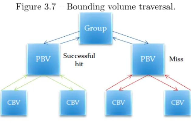
Figure 3.7 below shows an example of how the tree is traversed during picking. The group can be seen as a list with objects. PBV is a Parent Bound-ing Volume and CBV is a Children BoundBound-ing Vol-ume. Two objects are compared against a picking ray. The left side of the tree shows a successful hit on the parent volume and it continue to examine if its children are hit. The left side shows an unsuc-cessful hit on the parent BV and the children BVs are not tested at all.

Figure 3.7 – Bounding volume traversal.

Note: Group = some object list, PBV = Parent Bounding Volume, CBV = Child Bounding Volume 3.2.4 Collision Detection

A feature of the provided by the framework is that it is possible to move objects by hitting them with other objects. To reduce the number of computa-tions only the necessary objects are tested. It can be done by using a space partitioning structure such as a grid (see Figure 3.8). By connecting objects (scene graphs) to the intersecting voxels of a uni-form grid it is possible to limit collision detection by testing collisions on objects registered to nearby voxels instead of all other objects in the scene.

(12)

Figure 3.8 – Example of nearby cells searched during collision detection.

An early version of the framework used Axis Aligned Bounding Boxes (AABBs) for ob-ject/object intersection tests due to very fast col-lision detection and for rapid prototyping. Later on the scene graph structure was extended to sup-port rotations and the decision was made to use Oriented Bounding Boxes (OBBs). OBB/OBB in-tersection tests require more computations than AABB/AABB but can handle collisions with non-aligned boxes correctly which is impossible with AABB/AABB methods.

The following subsections describe the bounding volumes in this project including related algorithms and data structures.

3.2.4.1 Axis Aligned Bounding Boxes A common data structure in computer graphics is the axis aligned bounding box. The bounding box is used to encapsulate an object which often has a more complex shape. It is used mainly because of simple and fast intersection tests for both picking and object/object collision detection. Axis aligned means that the axes of the box are parallel to the world coordinate axes, or in other words have the same coordinate system.

Three AABB structures with intersection tests are described in the book Real Time Collision De-tection written by C. Ericson [10, c4, p78] where the AABB structure using a min point (amin_{) and a}

max (amax_{) point are used (as illustrated in Figure}

3.9). The extreme points are used to insert objects into a grid by transforming the coordinates to world coordinates and then decide in which grid voxels the min and max point are. All voxels covered by the AABB will be connected to the object by using a simple loop. The structure is not the most memory conserving representation of an AABB because of the six floating point values [10, c4, p79] but it is easy to work with and is excellent for fast develop-ment and testing purposes.

AABB { Point3d min; Point3d max; }

Figure 3.9 – A three dimensional AABB with its extreme points amin _{and a}max _{[2, c16, p729].}

3.2.4.2 Intersection Algorithms

There are two kinds of intersection tests that are used for AABBs in this framework. The first is the ray/box intersection test that is used for the picking feature. The second is the AABB/AABB intersec-tion test used for collision detecintersec-tion between objects and when inserting objects into the grid. Both in-tersection algorithms are described in the following sections.

AABB/AABB intersection

This algorithm is described in the book Real Time Collision Detection [10, c4, p79]. It is based on the Separating Axis Test (SAT) [2, c16, p744-745] to decide whether there is an overlap or not. Below is the intersection tests needed for detecting collision between two AABBs expressed in code.

int TestAABBAABB(AABB a, AABB b) {

// Exit with no intersection if separated // along an axis if (a.max[0]<b.min[0]||a.min[0]>b.max[0]) return 0; if (a.max[1]<b.min[1]||a.min[1]>b.max[1]) return 0; if (a.max[2]<b.min[2]||a.min[2]>b.max[2]) return 0;

// Overlapping on all axes means AABBs are // intersecting

return 1; }

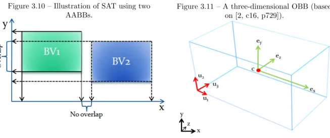
Figure 3.10 illustrates the separating axis method with two BVs in 2D-space. The BV’s sides are split into components (x, y) by projecting them against the world axes. In this case there are two AABBs so the projection doesn’t need any specific calcu-lations since the AABBs are already axis aligned. Only two axes needs to be tested in two dimensions to determine if there is an overlap or not. A collision succeeds only if the BV’s projected sides overlap on all axes. For three-dimensional AABBs it requires three intersection tests, one for every axis.

(13)

Figure 3.10 – Illustration of SAT using two AABBs.

RAY/AABB intersection

The RAY/AABB intersection test is a method that is based on the separating axis test [10, c5, p179]. The original method is described below [2, c16, p744-745]:

The parameters c and w are two points repre-senting a line. Variable h is the half vector of the box B.

RayAABBOverlap(c, w, B)

returns ({OVERLAP, DISJOINT}); vx = |wx| vy = |wy| vz = |wz| if(|cx| > vx + hx) return DISJOINT; if(|cy| > vy + hy) return DISJOINT; if(|cz| > vz + hz) return DISJOINT; if (|cy*wz - cz*wy| > hy*vz + hz*vy)

return DISJOINT;

if (|cx*wz - cz*wx| > hx*vz + hz*vx) return DISJOINT;

if (|cx*wy - cy*wx| > hx*vy + hy*vx) return DISJOINT;

return OVERLAP;

3.2.4.3 Oriented Bounding Boxes

An oriented bounding box can be seen as an exten-sion of the axis aligned bounding box. A difference is that an OBB can be aligned in any direction and thus be able to encapsulate objects with less unnec-essary space than an ordinary AABB as well as it can handle rotation. Figure 3.11 represents an OBB with three normalized u-vectors containing the cur-rent alignment of the box, a center point c and fi-nally a vector that holds the half-lengths (ex, ey, ez)

representing the size of the box along the u-axes.

Figure 3.11 – A three-dimensional OBB (based on [2, c16, p729]).

3.2.4.4 Intersection Algorithms

There are two kinds of intersection tests neces-sary for object/object collision detection and pick-ing to work with rotated objects. The first is the OBB/OBB intersection test which is very similar to AABB/AABB but has the capability of han-dling rotated boxes. The second intersection test is Ray/OBB which is used when selecting an object. The structure of the OBB can be seen in Figure 3.11.

OBB/OBB intersection

The collision detection between two OBBs is deter-mined by SAT which is built on the same principle as for AABBs. OBBs can be aligned in any di-rection and therefor require more intersection tests (see Figure 3.12). Up to a maximum of fifteen axis tests are needed to be able to decide if two OBBs are colliding or not. To avoid the zero-vector issue in calculations a small constant called epsilon was used.

(14)

RAY/OBB intersection

As the framework support rotated objects encapsu-lated by OBBs the Ray/AABB intersection method becomes insufficient. Possible solutions are to either entirely rewrite the intersection method to detect all possible ways the ray can intersect the box or a more efficient solution where the OBB is translated into an AABB and then perform the same tests as Ray/AABB with the same number of operations. The second method which is used in this project requires that the position and direction of the ray are transformed with the box. The ray intersection points on the box before and after the transforma-tions must be the same. This method is accom-plished by placing the OBB in origo and rotates it by using the inverse of the rotation matrix. It is now aligned with the world axes. As the OBB was placed in origo the ray position must be subtracted by the distance between origo and the OBB’s cen-ter point. To get the correct direction of the ray it is rotated by the inverse of the OBB’s rotation matrix. The transformations are illustrated in Fig-ure 3.13. The ray and OBB are now represented in world coordinates as a new ray and an AABB. The last step of the Ray/OBB intersection method is the Ray/AABB intersection method described in section 3.2.4.2.

Figure 3.13 – Ray/OBB represented as Ray/AABB.

3.3 Other Functions

3.3.1 File Formats

The supported format for loading 3D-models through the framework is the .3ds format. It is pos-sible to export models directly from Autodesk 3D Studio Max and it is preferred to save the model while in mesh mode since it will force every poly-gon to be represented as triangles. This framework as well as many game engines only support triangle meshes. Exporting a whole scene is not supported in a single call. Only one connected mesh at the time can be loaded by the framework. The .3ds file format comes with vertices and texture coordi-nates, normals are not included but can be calcu-lated through the framework.

3.3.2 Shaders

All objects can be styled with shaders, for example lightning methods such as per pixel phong light-ning and surface effects such as bump mapping. A shader can contain several effects which makes it very flexible. It is also possible to pass parame-ters from an application to the shader for real time effects. The motivation for using shaders is that they are highly programmable, easy swappable and that they can achieve a more lifelike and living en-vironment in 3D-space. Shader effects can be used to point out the differences in depth and the form of the objects. The current limitation of how many textures that can be used simultaneously is the tex-ture unit limit on the graphics card or OpenGL API. The framework supports one shader per geom-etry which is also easily swappable by using shader IDs (sID).

3.3.3 Text

The framework supports rendered text. By using SDL TTF (TrueType Font rendering library) text can be rendered onto a texture. It is possible to ren-der text directly to a quadratic polygon on screen but also to render to a texture. Rendering to a sepa-rate texture can improve performance since the tex-ture doesn’t necessarily have to be rewritten until the text changes. It is also possible to render text in 2D. By entering 2D-mode the framework sets up correct view matrices for 2D-rendering. If not using 2D-mode a texture rendered with text can be used on any 3D-object. All example applications in this project are using the Courier font (courier.ttf) of size thirteen with outlining.

3.3.4 Texturize

By using a function provided by the framework a picture can be loaded and converted to a texture in a single call. It is also possible to make a color trans-parent if needed. To be able to render textures with transparency the parameter ”GL BLEND” must be enabled through the OpenGL API.

4 Examples

This section describes the example applications, their implemented features and algorithms and data structures. These examples are mainly developed to show the flexibility of the framework and what it is able to do in its current state. The first ex-ample is a small Photo Viewer. Its main purpose is to show a collection of the framework’s capabili-ties in a single application. The second example is a scene viewer. It contains larger 3D-models and uses

(15)

more depth then the previous example. The frame-work also supports events when clicking or hovering objects. This is shown in the floating controls ex-ample where every 3D-buttons changes something in the scene. They also have the ability to collide with other objects if moved. The fourth example is more graphical and technical example and includes a texture blended 3D-model.

4.1 Photo Viewer

The first example application developed in this project was the Photo Viewer. It is built upon the framework and its main purpose is to test a large collection of features as a 3D-ZUI. The application is designed as a Photo Viewer not very different from two-dimensional software. The biggest differ-ences are in navigation, interaction with real 3D-objects, graphics with depth and real time effects, floating photos with the ability to collide.

4.1.1 Features

The currently implemented features such as arc ball, select and drag, grabbing, throwing, naviga-tion, zooming and collision detection are explained in the following sections.

4.1.1.1 Arc Ball

A common implementation of an arc ball was inte-grated to be able to rotate objects, to decide the rotation of a sphere by calculating how two click rays intersects with a sphere. Figure 4.1 shows that A and B are rays (calculated from the mouse click), v and u are vectors from the spheres center to ray A and B. By calculating the cross product of u and v (u x v ) we get the w vector which is represent-ing the rotation axis. By usrepresent-ing simple mathematics the angle a can be achieved which represents the rotation around the w -axis. An arc ball support rotations in any direction, any degree around every axis and it is possible to click on it from from every position in 3D-space.

Figure 4.1 – Arc Ball

4.1.1.2 Select and Drag

An important feature is select and drag, it means that you can select a photo and interact with it such as moving the object by using the mouse cursor (see Figure 4.2).

Figure 4.2 – Moving a photo in any direction.

4.1.1.3 Grabbing

Grabbing is a feature to ease the navigation when browsing photos. Simply grab the background (or grid) and drag it in any direction as in Figure 4.3 and then release as in Figure 4.4.

Figure 4.3 – Grab and drag.

(16)

4.1.1.4 Throwing

A feature that was implemented into the Photo Viewer example application is throwing. Throwing is achieved by selecting and dragging a photo with the mouse and then releasing it while moving (see Figure 4.5–4.7). The photo will continue to move with initially the same speed as the mouse cursor but will later slow down due to a friction assigned to the transformation node of the objects. This feature was implemented to make interaction more real as a paper photo on a table. It can be useful to quickly move photos out of the way or to group them by throwing them to a specific place on the screen or usable area. If collision detection is en-abled other photos will react differently depending on the speed of the colliding photos.

Figure 4.5 – Drag photo.

Figure 4.6 – Release photo while dragging.

Figure 4.7 – Photo now has its own velocity.

4.1.1.5 Navigation

One of the most critical features of a 3D-ZUI is the navigation system. There are various navigation techniques implemented. One of them is a steering technique called WSAD which navigates the cam-era in different directions, W is forward, S is back-wards, A is left and D is right. Keyboard arrows and NUMPAD is also supported. It works in the same plane as the wall and supports eight directions incl. diagonal directions. NUMPAD 8 navigates the camera up, 2 down, 4 left, 6 right, 7 up left, 9 up right, 3 down right, 1 down left. To restore the view to the center there are two keys available, either C or NUMPAD 5 or by right clicking and selecting reset camera in the menu.

4.1.1.6 Zooming

As this application is built as a zoomable user in-terface it also has zoom capabilities (see Figure 4.8– 4.11). The feature zooms towards the direction the mouse cursor currently is pointing at which makes it easy to select the area to enlarge. If you are zooming the upper left corner you will end up at the point you are pointing at. Zooming out at the same point will take you back along the same path. The zoom feature is also supported using the scroll button on the mouse and keyboard sign (+) zooms in and (–) zooms out. Double clicking on a photo it enters full screen 2D-mode with black background.

Figure 4.8 – Zoom level I.

(17)

Figure 4.10 – Zoom level III.

Figure 4.11 – Full screen zoom.

4.1.1.7 Screen Tracking

Screen tracking is another kind of navigation fea-ture often seen in strategy and role playing games. By hovering tracking borders with the mouse cursor the screen will pan in the same direction (see Figure 4.12–4.13), for example hovering left tracking bor-der it will take you to the left and by placing the mouse cursor in the upper left corner it will take you in that direction. This can be an optional nav-igation system to the keyboard or can be used at the same time. For example when a photo is to be moved outside screen space it’s possible to drag the photo over the tracking border and the view will pan in the same direction. The further the cursor is passing the borders the faster the screen will pan.

Figure 4.12 – Tracking Markers.

Figure 4.13 – Tracking Borders.

4.1.1.8 Colliding Photos

Another feature that was implemented was Collid-ing Photos which means that no photo can overlap another photo as long as collision detection is en-abled. If you drag a photo into another the second photo will be pushed out of the way. If the sec-ond photo collides with another and another also they will be pushed out of the way, a chain reac-tion that is. If a photo no longer is grabbed or if it is thrown away it will react to collisions as any other photo. If a photo in some way is passing out-side the wall it will be transferred to the opposite side automatically. This feature can be deactivated if necessary. Figure 4.14–4.16 are rendered screens from the Photo Viewer showing a high velocity ob-ject bringing chaos when causing a chain reaction.

Figure 4.14 – Giving a photo high velocity.

(18)

Figure 4.16 – Chain reaction resulting in chaos.

4.1.1.9 Menus

The photo application uses menus. By right clicking with the mouse cursor in an empty space brings up a list of global setting that can be changed. Right clicking on a photo shows available functions for the specific object type, like rotation.

4.1.2 Algorithms & Data Structures The following two sections explain the algorithms and data structures used in the Photo Viewer, fea-tures that is not fully supported or part of the framework.

4.1.2.1 Grabbing/Select and Drag

The Photo Viewer’s ”grabbing” and ”select and drag” feature are easy to implement for two-dimensional space, although for three-dimensions there are some differences. Due to the perspec-tive view (non-orthogonal view) distances between points are not constant in three dimensions as in two. For example if you select and drag a photo that is near the screen the object will travel at the same speed as the cursor, which is similar to what happens in two dimensions. However, if you do the same with a photo far away it will need to travel much faster to keep up with the cursor. The prob-lem is that the distances further away from the cam-era are not matching the distances between screen coordinates (mouse points) which is caused by the Field of View (FOV) value used to simulate the eye lens effect. The FOV parameter alters the view vol-ume and makes objects further away smaller. Let’s take a look at the problem illustrated in Figure 4.17 and 4.18.

Figure 4.17 – Orthogonal view volume v1 where c1 and c2 are click rays.

Figure 4.18 – Perspective view volume v2 where c1 and c2 are click rays.

Figure 4.17 shows an example where the click rays c1 and c2 passing the orthogonal view volume v1 have the same distance when going in (d1 ) and out (d2 ), here would calculations for two dimen-sions suffice.

In Figure 4.18 it is shown that the distance be-tween the rays grows the further away from the starting point it gets. Distance d3 is measured in the starting point and d4 is measured deeper into the volume, compared to no difference between d1 and d2 in Figure 4.17 the difference is huge. A larger field of view means greater distance between end points.

This issue can be avoided by using picking pro-vided by the framework and setting up a virtual plane as described below:

Phase 1 - Click and hold:

1. Get the position the picture is located at (frameworks picking algorithm).

2. Use the vectors from camera and set up a par-allel 2D-plane at the picture location. Phase 2 - Hold and drag:

1. Send a new ray against the plane and get the intersection point

2. Calculate the distance between the first pic-ture intersection point and the second plane intersection point

When knowing the mouse coordinates and the dis-tance to where the picture is located it is easy to set the picture’s new position. Grabbing and moving view is another navigation technique that is based on the same idea as when moving objects but is using grid planes and not pictures as target in the first phase. It basically navigates the user in the opposite direction of the dragging direction. 4.1.2.2 Throwing

To be able to throw a photo then objects must have velocities. Velocities are supported by the framework through transformation nodes. Throw-ing is also heavily dependent on the select and drag algorithm since the photos are placed on a cer-tain depth. The Photo Viewer application uses the

(19)

framework to get and set the photo position. Ve-locity of the photo is dependent on the mouse and the delta vector of the photo movement is stored as a velocity in a list. The list can store any number of velocity vectors but in this example application it is limited to a few. Throwing is done in three steps, clicking, dragging and dropping. The first click gives a starting point. Dragging gives veloc-ity samples while the user is moving the photo with the mouse cursor. Dropping gives the photo a final velocity which is a median of the collected veloci-ties. The median of the collected values are used to smooth the outcome, otherwise it would be possible to get zero or extremely fast velocity if any jump in movement occurred.

4.2 Scene Viewer

The scene viewer example is more focused on us-ing three dimensions such as several larger models with textures and shader effects. This section also includes how models are constructed and loaded by the framework as well as some screen shots from the original scene in Autodesk 3D Studio Max10.

Figure 4.19 below is a screen shot from the scene viewer. The scene is built of multiple scene graphs that are linked into the uniform grid. The camera in this example is not restricted which makes it pos-sible to fly around and look from every angle of the scene.

Figure 4.19 – Models loaded into the scene viewer.

4.2.1 Models

Most models in the scene viewer are constructed from several meshes, textures and nodes that are linked to a single scene graph, which means that all connected parts will move if the scene graph object moves. It is possible to assign multiple objects the same texture and shader ID (tID and sID ). Every mesh has its own transformation node which makes it possible to move and rotate them to the wanted position. Below is a list of meshes and materials for the statue in Figure 4.19.

1. Body mesh, dark shiny cloth material. 2. Left and right arm mesh, dark shiny cloth

tex-ture.

3. Hat mesh, dark shiny cloth texture.

4. Left and right leg mesh, gray shiny cloth tex-ture.

5. Head mesh, white shiny stone texture. 6. Left and right hand mesh, shiny stone texture. 7. Left and right feet mesh, shiny stone texture.

4.2.2 Modeling

Figure 4.20–4.23 below are a four screen shots taken from different angles of the original scene while be-ing modeled in Autodesk 3D Studio Max. Each model of the scene was texture mapped and con-verted to a mesh of triangles before being saved to the .3ds file format. Note that lights and material effects such as blinn and phong lightning models and their settings are not saved to the .3ds file for-mat, these has to be set manually after being loaded by the framework. All polygons have the form of a triangle in mesh mode, which is a requirement when loading through the framework.

Figure 4.20 – Original scene from top.

Figure 4.21 – Original scene from left.

(20)

Figure 4.22 – Original scene from front.

Figure 4.23 – Original scene from perspective view. Texture mapping in progress.

4.3 Floating Controls

This scene is built up by three frames viewing dif-ferent pictures and three buttons. The purpose of this example is to show that the framework sup-port event handling and that textures easily can be swapped through node search and change of texture ID. There are three events which are connected to the geometry nodes of the buttons. Clicking any button except the middle one will loop the pictures viewed by the frames back and forth. The middle button will close the application. Every geometry node can hold user made events that are triggered if the object is hit during a ray intersection test. All triggered events are caught in the event loop and from there it is possible to read information passed from the node. By using a list of texture IDs and it is possible to step forth and back in the list for the desired effect. Below is a small code example:

if(event.zui.user.code==UEGEOMETRYCLICK){ int id = *(int*)event.zui.user.data1; int in = *(int*)event.zui.user.data2; SceneGraph* sg = ZUI_GetObject(id); if(sg){ MaterialNode* g = (MaterialNode*) sg->GetNodeByName(SGMATERIAL); GLint ta = g->texInfo[0].GetTexture(); (change texture based on id & in here) g->texInfo[0].SetTextureID(ta);

} }

The event that is sent to the event loop can be cre-ated by the piece of code below. The first row allo-cates memory for the new event e while the second is a user defined code to be able to distinguish it from other events in the event loop, the third sets the type to user event which is an unused range in SDL. The next two rows set two integers where the first is a known scene graph id which is supposed to change when the event is received. The second one is the ID of the node in the selected scene graph to be found or changed. The ID has to be assigned to the node manually and in this case it is called SGMATERIAL and has a value of one. The last two rows are pointer assignments which makes it possible to read the values in the event loop.

ZUI_Event* e = new ZUI_Event(); e->zui.user.code = UEGEOMETRYCLICK; e->zui.type = SDL_USEREVENT;

*sid = 4; // allocated int*

*inc = SGMATERIAL; // allocated int* e->zui.user.data1 = (void*) sid; e->zui.user.data2 = (void*) inc;

Below is a short piece of code showing how to assign name or search value of a material node. The first row allocates memory for the new node, the second assigns which texture to use through the integer textureID, it also assigns the texture unit which is the first one and the name of the texture in the shader to pass it to is named texture1. The third row assigns which shader to be used. In this case the loaded shader is located on the third place in the shader container. The last row needs to be set if it should be possible to search for the node by its name or id, which in this case is SGMATERIAL with value of one.

MaterialNode* mn = new MaterialNode(); mn->InitializeTexture

(textureID, 0, "texture1"); mn->InitializeShader

(sc->GetShaderObj(3)->shaderProgramID); mn->SetName(SGMATERIAL);

(21)

4.4 Texture Blending

This is a small example containing a 3D-model with texture blending (see Figure 4.25–4.28). Texture blending is achieved by assigning three texture IDs on three different texture units to a single mate-rial node. It is possible to link the three textures to a shader where the first and second are different materials and the third is texture mask or blending texture. The texture mask is a gray scale image and decides if texture one or texture two should be vis-ible at every fragment. Black means the fragment color of texture one and white means the fragment color of texture two, gray means equal amount of color from both textures.

Figure 4.25 – White stone texture.

Figure 4.26 – Black stone texture.

Figure 4.27 – Texture Mask.

Figure 4.28 – Result: white + black + mask.

5 Results

As there still are many performance related algo-rithms to implement to see the framework as com-plete it would be wrong and misguiding to mea-sure performance at this point. The two major data structures the uniform grid, the scene graph as well as algorithms implemented into the framework are well motivated for their purposes: performance and flexibility, which is what the first section is about.

During this project a small pilot study was made to collect information by evaluating an early proto-type of the Photo Viewer, the results are presented in the second section.

5.1 Performance

The choice of data structures and algorithms for the 3D-ZUI framework turned out to work well for the example applications. The scene graphs are flexible and easy to extend if needed due to independent behavior and object oriented design, these were the most important design goals of this project. When many objects are loaded into a 3D-ZUI it is not enough to use a brute force algorithm for picking and collision detection. To improve performance of the 3D-ZUI a three-dimensional uniform grid was implemented into the framework. The theoretical performance improvement comparing to not using a grid at all for picking and collision detection is huge. Exactly how many objects the framework can han-dle remains to see as it greatly depends on the grid-, voxel- and object size [11]grid-, how these structures combined affects performance is not yet measured in numbers and is listed as future work.

When looking closer on theoretical performance for ray traversal the worst case traveling path for a ray through a two-dimensional uniform grid of size 6x6 is from voxel (0, 0) to (5, 5). For a cor-rect and precise path it requires traversing through 11 voxels using the traversal algorithm described in section 3.2.2.1. The best case is 1 voxel if the ray

(22)

starts for example in voxel (0, 0) and is pointing in a negative direction or that voxel (0, 0) is holding the wanted information. A brute force algorithm would always end up passing 36 voxels which is about 3.3 times slower and this is for the two-dimensional al-gorithm only. Picking without the grid would have to loop through all objects for every pick instead of the ones that are placed nearby the click ray. Dif-ferent kind of applications may use a much larger grid with varying voxel sizes. The Photo Viewer ap-plication grid is set up to about 5000 voxels which is a rather small zoomable user interface that isn’t utilizing the depth very much. The 3D-DDA algo-rithm by John Amanatides and Andrew Woo [3] is considered a fast and memory conserving algorithm. The same principle as for ray traversal applies for object/object collision detection. The uniform grid is used for the collision detection to reduce the number of objects tested against each other. A spatial partitioning structure is very effective per-formance wise when it is encapsulating many ob-jects. The grid is accelerating collision detection by searching the voxels the objects are registered in to quickly find nearby objects. Objects that are not registered in the voxels are not tested for intersec-tions. In an application with 5000 objects there might be only 10 that are colliding at the same time in different places. Since an object otherwise has to be tested against all other objects, it would give about an average of 25 million object/object intersection tests. The grid also needs to relink moving objects in the grid which requires compu-tations. The framework is using AABBs to insert and remove objects from the grid. This method is very fast and does not require any intersection tests but some objects may be registered in more voxels than necessary. It is important to balance the grid size and voxel size for the objects in the applica-tion for optimal performance [11]. Too large vox-els would increase the number of intersection tests with nearby objects while too small voxels would increase the time spent on relinking the grid, voxel search around objects and also ray traversal in the grid.

The scene graph is structured as a BVH which means that all BVs in the structure don’t need to be tested and by doing so it becomes fast to traverse and test for intersections. The current version of the framework allows BVs to overlap which should be kept in mind when building the scene graphs. The scene graph supports dynamic models at the time and it is possible to move nodes further down the tree. BVs does not automatically rebuild in the current version of the framework so picking will only work correctly on static models or manually updated BVs. This is also one of the reasons why switch nodes are not yet implemented.

It is possible to improve performance even fur-ther. Some limitations that were expected and that also appeared during extreme testing were related to memory and rendering power. These issues are known and solutions are available. Two kinds of culling, a texture manager and also a technique called LOD (Level of Detail) are currently being looked into and are listed as future work.

5.2 Pilot Study

An early prototype of the Photo Viewer was evalu-ated by a small group of persons. The purpose of this pilot study was to get feedback and guidelines by investigating how people felt about the concept and at the time implemented features. The test ap-plication had several predefined photos that were loaded when the application was started. There were no restrictions of how to use the application. After the test run the users were asked to fill in an evaluation form containing questions about how they experienced the Photo Viewer and its current features.

Most questions asked were directly related to the Photo Viewer (framework) and features. The scale 1-9 was used so the user could give an accu-rate answer to each question. A summary of the evaluation is represented by a table (see Table 1). The purpose of the table is to show the average re-sponse by using a scale of 1-9 for every question. A score higher than 5 is good and a score lower than 5 is not as good, a value of 5 is neutral.

Table 1 – Summary of evaluation.

QN TYPE AVG Q1 Age 44 Q2. Yes/No 3.3 – – – Q3. Bad/Good 9.0 Q4. Bad/Good 8.3 Q5. Bad/Good 8.3 Q6. No/Yes 8.7 Q7. Bad/Good 9.0 Q8. Bad/Good 8.7 Q9. Bad/Good 8.0 Q10. Yes/No 7.7 Q11. No/Yes 7.7 Q12. No/Yes 8.7 Q13. No/Yes 5.3 Q14. No/Yes 9.0 – – 8.2

The application and evaluation form was handed out to a small group of test users. Below is a quick summary of the results.

Question one (Q1) and Q2 which are age and experience of similar applications were asked to be