Marginal cost pricing of scheduled transport services

49

Marginal Cost Pricing of

Scheduled Transport Services by Jan Owen Jansson

Reprinted from Journal of Transport Economics and Policy No. 3. Sept. 1979

\ Marginal Cost Pricing gif

Scheduled Transport Services

Jan Owen Jansson \

,

i Reprinted from

A,

SCHEDULED TRANSPORT SERVICES

A Development and Generalisation of Turvey and

Mohring s Theory of Optimal Bus Fares

By Jan Owen Jansson*

1. BACKGROUND, PURPOSE AND MAIN IDEA

A useful general price theory for the whole transport sector is dif cult to imagine, in View of the many important differences within the transport sector in both demand and supply. The most common approach is to deal separately with each mode of transport. This is the most natural division from a transport technological point of View.

Another division of the transport sector can be more adequate from an economic point of view. Instead of considering the pricing problems of each mode of transport separately, it seems in many respects more appropriate to divide transport price theory into these three departments:

Price theory for track (road, rail, fairway) services

Price theory for services rendered at passenger and freight handling terminals . Price theory for services rendered by transport vehicles, or simply transport services .

The third department should, in turn, be divided into the subdepartments of the charter market and the market for scheduled transport services . The present discussion is about marginal cost pricing of scheduled transport services sts for

short.

The vehicles producing sts are charged either a price or an accounting cost for the use of tracks and terminals. Where the track and terminal costs appear as charges on the vehicles, but it can be expected that those charges do not equal the marginal costs of making use of the tracks and terminals concerned, a problem arises of limita-tion of an analysis of marginal cost pricing of sts. The present analysis does not go into this problem. It is in line with the above suggested division of transport price theory to delegate the responsibility for a total optimum between experts of each of the three departments, so to speak. For modes of transport like the railways where the tracks and terminals are owned by the producer of transport services, it could

M.G. PRICING OF SCHEDULED TRANSPORT jan Owen jansson be argued that a discussion of MC-pricing of the transport services should also go into the problems of costing or internal pricing of the constituent track and terminal ser-vices. This is not done here. One point of the suggested division of transport price theory is that the particularly complicated pricing problems facing railway

com-panies and other vertically integrated transport enterprises will be separated in such

a way that theoretical advances in other areas can be put to the maximum use. For example, the problem ofrail track costing is more akin to the problem ofroad pricing, and the problem of railway terminal costing has more in common with the problem of port pricing, than with the problem of costing and pricing of rail transport services.

Apart from railway passenger transport, economists have not been much interested in the pricing problems of scheduled transport undertakings. Even for railway trans-port pricing, the vivid interest shown in the rst halfof this century by leading econo-mists like Wicksell, Cassel, Pigou, Taussig, Hotelling and Dessus seems to have faded in modern times. The reason for the lack of interest of modern economists cannot be that the consensus of opinion has been attained on a method of Optimal pricing of scheduled transport services. At least in the general debate, suggestions of reforma-tion of public transport pricing policy range from the applicareforma-tion of zero prices to self nancing full-cost pricing.

However, a path-breaking contribution, which should cause a renaissance of the interest of economists in this field, has been made by Ralph Turvey and Herbert Mohring (1975). I think they have located exactly where earlier contributions went wrong, and why it never seemed to be possible to arrive at a consistent theory of optimal pricing of scheduled transport services:

The right approach is to escape the implicit notion that the only costs which are relevant to optimisation are those of the bus operator. The time-costs of the passengers must be included too, and fares must be equated with marginal social costs. (Turvey and Mohring, p. 280).

The main problem considered by Turvey and Mohring was, in their own words, to nd out what marginal cost pricing of bus services consists of , but also to give an indication of what the nancial result of optimal bus fares would be. The present

paper follows up and seeks to generalise some of the ideas put forward by them to the

whole sector of sts. It is argued that the crucial (for optimal pricing) characteristics of urban bus services reappear in one form or another for all scheduled transport of passengers and freight alike.

A bird s eye view of every system of scheduled transport reveals a basic similarity: Regardless of the mode of transport, whether the vehicles are borne on a road, a rail track, water, or air, the vehicles are moving to and fro along given routes, making halts at more or less regular intervals for loading/unloading at predetermined stops . However, for every mode of transport the size of the vehicles employed can vary in a very wide range. And, roughly speaking, there is a one-to-one trade-off between size and number of vehicles.

From an economic point of view, the salient feature is that there are signi cant economies ofnumber of vehicles serving a given geographical area, and equally import-ant eeonomies of vehicle size. The number economies are manifest in the user costs, while the size economies exist in the producer costs. The number economies have to do

with the access to sts, and are normally re ected in both the frequency of service and the density of service.

Given the size and load factor of buses, it is clear that the frequency of service will be roughly proportional to the demand. A symmetrical source of variation in user cost is the positive correlation between the accessibility in space ofsts and the density of demand. A study of maps of networks of railways, airlines and bus services as well as roads will give a vivid impression that the more sparsely populated a region is, the more coarse-meshed the network will be. Similarly, the density of the shipping lines connecting two continents is strongly correlated with the seaborne trade volume per mile of coastline.

Generally, the average feeder transport distance will become longer and longer as the network becomes more coarse-meshed or the density of sts lower. Therefore, the costs of users of scheduled transport services for transporting themselves or their shipments to and from the sts stations can be expected to be related to the density of demand, in much the same way as the user costs of infrequency of services are related to the density of demand.

The main transport policy angle of the matter is that the coexistence of signi cant economies of vehicle size and economies of vehicle number makes the sts sector a pronounced decreasing-cost industry ; that is, the application of social MC-pricing will result in a nancial de cit. This conclusion is particularly remarkable in view of the fact that the charter markets for sea, air and road transport alike, where basically the same sort of vehicles Operate as those engaged in scheduled transport, , are commonly regarded as some of the most perfectly competitive markets in

existence.

The basis for the discussion is the following model of an abstract mode of sts, viewed in a bird s eye perspective in order to keep hold of the common characteristics ofsts, and not get lost in speci c details.

2. GENERAL MODEL OF AN ABSTRACT MODE OF SCHEDULED TRANSPORT SERVICES

Just as for investment problems of sts, the understanding of optimal pricing of sts needs a system cost approach. This implies:

1. equal treatment for the transport service producer costs and the transport service user costs; and

2. that a network ofscheduled transport services should be considered, rather than an individual link in a network.

In cost/bene t analyses of transport investments the method of translating bene-ts to users into user cost savings has a long tradition, particularly in road investment appraisals. In the eld of urban public transport, the CBA of the Victoria Line from 1962 was a pioneering contribution (Foster and Beesley (l963)).

In transport pricing, the importance of treating producer costs and user costs on a par has not been widely recognised outside the extensive literature of optimal road user charges. As has been mentioned, in the wide eld of scheduled transport it has only very recently been realised that the principle of marginal cost pricing is

prac-M.G. PRICING OF SCHEDULED TRANSPORT jan Owen jansson tically impossible to apply correctly unless all user sacri ces and efforts are, at least conceptually, treated as costs on a par with the producer costs. By the following model it Will also be shown that the level of optimal sts prices comes out differently when a sts system rather than an individual line is considered. '

The model seeks to describe the main effects on producer and user costs ofdifferent designs ofa system ofsts. The system is de ned by a given geographical area, which is traversed in different directions by a smaller or larger number of transport vehicles plying xed routes according to pre-announced time tables. The aggregate output of sts per unit of time, QJ is given by the production function (l) below. A main simpli cation of the analysis is that cyclical uctuations in demand are ignored. An alternative interpretation of the assumption of a homogeneous unit of output is that it represents a composite unit including oc units of peak output and ,B units of off-peak output.

The production function is supplemented by a function for the total producer costs (2), and a function for the total user costs (3).

Then

Q = ¢NHV,

<1)

where

H = H<X>,

M

and

V=wxn¢»

aw

TCpmd = NZ, (2) where

Z = g(X) + PT + 6(X)-

(221)

T "ser = QMC/Ö, N, V)-

(3)

Q = transport volume

(,b = load factor or occupancy rate

N = number of vehicles

H = holding capacity of a vehicle V = overall speed of vehicles TCpmd = total producer cost T "ser = total user cost

X = vehicle design vector

Y = current input vector (fuel, cargo handling labour, etc.) Z = total producer costs per vehicle-hour

g(X) = overheads, capital and crew costs per vehicle-hour ]) = current input prices

c(X) = track and terminal charges

/z = total user cost perjourney (passenger trip or freight transport).

Total output is the product of the load factor or occupancy rate, the number, the holding capacity, and the overall speed of the vehicles in the system. By overall

speed is to be understood the ratio of the distance travelled per operating year to the total hours of Operations, including all the time spent in handling passengers or freight at terminals as well as the time spent in hauling. The holding capacity H and overall speed Vare determined by a number of primary factors of production. These factors can be divided into two distinct classes: on the one hand there are a number of vehicle design variables such as the hull dimensions of a ship and the engine power, and on the other hand there are some current inputs such as fuel. The holding capacity cannot be varied by varying the current inputs. The overall speed is a function of the vehicle design, as well as of the actual input of fuel and labour for freight handling at terminals. A third determinant of V is the load factor, (15. This factor is a somewhat unconventional factor of production . It appears both as an argument in the V-function and as a scalar of the production function. Its latter role is self explanatory: the transport capacity is given by NH V, and, in order to produce transport output, the capacity provided has to be utilised by passengers or freight. If the capacity were independent of the actual rate of utilisation, the output would be strictly proportional to (,b. This is, however, not true in general. It is not that the load factor affects the hauling speed very appreciably. This effect is in fact almost negligible, at least so far as passenger transport is concerned. It is, in the rst place, the handling time that depends on the load factor. Given the average trip length, the more passengers a bus carries, the longer the time at stops will be, ceteris paribus. In freight transport this effect can be quite strong. This is particularly true in break-bulk cargo shipping, where the ships often have to spend more time in port than at

sea (unless the load factor is abnormally low).

In the V function gb is consequently a factor which has a negative effect on output. The total effect ofqb on Qis, of course, positive. The partial elasticity of Qwith respect

to gb equals 1 plus the partial elasticity of the overall speed with respect to (b.

E0, = 1 + EV,

(4)

E% is negative, but its absolute value is normally much less than unity.

The total factor costs of the producer ofsts are written as the product ofN and the cost per vehicle hour Z, which consists of the costs of the current inputs, pY, and the costs of all those factors which are xed in the short run, including overheads , vehicle capital and crew costs as well as track and terminal charges. These charges are assumed, for a given type of vehicle, to be proportional to the time of use.

A common procedure in transport service costing is to make a sharp distinction between the traffic operation costs (including vehicle capital and crew costs) and those costs which are not directly associated with the traf c operations, that is, the overhead costs. It is argued here that this sharp distinction is overdone and, when it comes to marginal cost calculation, can be quite misleading. The overhead costs constitute, of course, a notorious problem in all costing, and deserve special dis-cussion here. However, in order not to break the flow of the main argument, this discussion is postponed to the last section.

Given the location of activities generating demand for sts, the users own contri-butions to the ful lment of this demand can be summarised by these four efforts: l. Cate/ling the vehicles producing sts, involving feeder transport in the

M.G. PRICING OF SCHEDULED TRANSPORT jan Owen jansson 2. Queuz'ngl for these vehicles on occasions when there is excess demand;

3. Going by the vehicles.

So far as freight is concerned, a fourth cost can be very important, namely: 4. The direct effort of loading and unloading.

At this stage the only necessary speci cation of the user cost function is to mark that in the rst place gb, N and V are important determinants of the corresponding costs. The load factor is the principal determinant of the queuing costs. In the case of passenger transport, a high occupancy rate can also cause crowding costs , that is, raise the cost of travel time. Given the overall speed, the number of vehicles in the system N determines the accessibility of service in time and space. A given eet of vehicles can be allocated to a large number of separate lines to maximise the accessibility in space or to a relatively small number of lines to give a high fre-quency of services. If the former course is chosen, the feeder transport costs will be low, but the actual or potential waiting time cost will be high, and vice versa if the latter course is chosen. A generic name for all user costs caused by the necessarily imperfect accessibility of sts is catchment costs .

The appearance of the third argument in the user cost function the overall speed V is explained by the facts that the transport time cost is inversely propor-tional to V and that, given the number of vehicles employed on a particular route, the frequency of service is proportional to V.

This concludes the presentation of the general model. In what follows, the model will be put to use to discuss the contents of the optimal price ofsts in terms of marginal costs. On the basis of this discussion, it is possible to get a rough idea of what the

nancial result of optimal pricing would be for different categories of sts.

3. THE OPTIMAL PRICE IN TERMS OF MARGINAL COSTS MC-pricing of transport services, as well as of other services where the user cost is a non-negligible social cost component, implies that the optimal price P should con-sist of two items the cost effect on the producer, and the cost effect on the original users of the facility concerned, of another unit of output. The following expression is the most general formulation of the optimal price, or pricing-relevant cost as it may be preferable to call it.

d d

P = __ chrod +

dQ<

> QdQ(

Acuser .

>

<>

5

This general formulation of the pricing-relevant cost does not commit us to any decision on the relevant run for pricing, that is, on which factors of production should be assumed to be variable.

Turvey and Mohring discussed optimal bus fares in terms of short-run marginal

1The queuing may be conspicuous or latent as in the case where seat reservations are made before-hand. The disadvantages for the passengers of (e.g.) an airline of sometimes nding that the desired

costs (SRMC). By the present model their discussion is generalised, and a certain vagueness ofde nition can be clari ed. After that we present an alternative medium run formulation ofthe pricing-relevant cost, which it will be argued seems more useful for sts pricing in practice. It will be shown, nally, that under the normal ef ciency conditions P, as stated above, comes out the same no matter which run it is calculated for.

3.1 The pricing-relevant cost in the short run

In Turvey and Mohring (1975), as well as in an earlier paper on bus fares by Mohring (1972), only the right-hand component of (5) is recognised as pricing relevant, or, in other words, only various costs imposed on fellow passengers enter the optimal price. In the present model this corresponds to assuming all producer inputs to be xed, allowing only the occupancy rate gb to vary. Under this assumption the general expression for the optimal price (5) takes this shape:

((a/z

ÖVÖ/z d

Q 55 + 53% (15>

0/2

aVa/z

PSR =

_av

=

_Ög!)

+ ¢.

_aqsaV

-

<6)

(NHV + (Ml/Hag)

Two separate imposed costs can be distinguished: one is the crowding and/or queuing cost caused by raising the occupancy rate, represented by the left-hand term, and the other is the imposed handling time cost. As seen from (6), the latter effect on the user cost of raising d) is working via the negative effect on V of an in-crease in gb.

The crowding or queuing cost appears in one form or another for all modes ofsts. On buses or trains where a number of standing passengers are allowed, the average comfort will fall as soon as all passengers cannot be seated. As the number ofstanding passengers grows the discomfort will be aggravated, and when the passengers are packed like sardines conditions are hardly endurable. In the C pure crowding case it can, a priori, be assumed that except in very exceptional cases buses or trains should not be so full that/some passengers have to be left behind. (It is probably not optimal to operate at such a high rate ofuse ofholding capacity that some passengers Of their own will choose to wait for the next bus/train in the hope that it will be less crowded.)

There is also a pure queuing case where no crowding costs are present. In freight transport the pure queuing case is applicable, provided only that the risk of damage does not increase as the load factor goes up. In passenger transport it may be argued that the pure queuing case is applicable, too, in all cases where no standing is allowed. However, even though everybody has got a seat, most travellers probably consider comfort to be more or less impaired by a high occupancy rate.

The imposed crowding cost appears as an increase in the cost of travel time. A separate effect of raising the load factor/occupancy rate is that, ceteris paribus, the transit time will go up. Given the transport capacity provided, more passengers or freight means that more time has to be spent in cargo handling or in boarding/ alighting of passengers. In Turvey and Mohring s discussion of optimal bus fares the boarding/alighting time cost imposed on fellow passengers plays a main role,

M.G. PRICING OF SCHEDULED TRANSPORT jan Owen jansson and in Mohring s earlier paper (1972) on urban bus transport it is assumed to be the Only pricing-relevant cost.

From one point ofview it may seem appropriate to reserve the epithet short run to the costsjust dealt with, which arise when all producer inputs are xed, and only (15 is a variable. This is in the closest analogy with the short-run costs of (for example) road use or the utilisation of other xed facilities. From another point of view this does not appear as the most appropriate convention. From the point of view of the actual decision-making in a sts undertaking, the xz'ng eft/ze schedule can be considered to be the most important dividing line between questions of short-term operations and longer-term policy matters. Some of the most typical short-term questions concern the problem how the schedule is to be kept in the face ofvarying conditions, including random uctuations in the demand from one day to another; that is, how to maintain a reliable service.

In this light Turvey and Mohring s short-run marginal cost concept appears as a half-measure. They assume the total bus-hours to be xed, but not that a xed schedule is adhered to. An increase in the demand will in their short-run cost model cause time losses for the original passengers through a lengthening of the time at stops. This must imply either that the bus line schedule is being adjusted in accord-ance with changes in the expected demand, or that the important desideratum of reliability of the service is ignored. For the former alternative (where the schedule is assumed to be a variable) the short run is not a very tting designation. If the schedule can be adjusted, one mightjust as soon assume (e.g.) the vehicle input to be variable. To abandon reliability is to my mind an unrealistic representation of the behaviour of most sts undertakings (including urban bus services).

The very idea of sts is that a published time-table is to be maintained even under adverse circumstances. The main precondition for this is that the schedule is not made too tight, but that a time loss incurred at one stage of the round trip can be made up subsequently by speeding up operations. With reference to expression (6) for P, this means that the imposed handling time cost is zero in the short run. As long as the schedule is xed, the potential handling time costs caused by additional traf c will be reflected in various schedule-keeping costs . This is a generic name for a variety of minor cost items which make themselves known on the occasions when the actual demand is greater than usual.

For example, in liner shipping, when an unusually large quantity of cargo which is dif cult to handle is presented for a particular sailing, the time lost in the handling operating will be regained by reducing both the dead port time and the cruising time on that particular sailing. By working overtime in port the ship s idle time can be substantially cut, and the time at sea can be reduced by steaming at maximum speed. This is obviously not done with impunity; the tighter the schedule is, the higher will the cost be ofsaving a day in port or at sea. In passenger transport the main possi-bility to regain time when the boarding/alighting time has been unusually long is to increase the running speed. In urban bus transport another frequently used method of time-saving when behind schedule is to cut the time at stops to the detriment of the comfort of passengers. The time per stop can be shortened by abrupt stopping and starting, by rushing boarding and paying passengers, by ignoring the woman with the pram, by not waiting for the late-comer running to catch the bus, etc.

normally steam ahead of schedule, but keeps the schedule by going slowly and avoiding all overtime work. In passenger transport it is particularly important not to frustrate travellers by early departures.

In the present model this means that an additional constraint should be imposed, namely, that the overall speed Vshould be assumed to be given in the short run. In that case the existence of some current inputs T has to be recognised. Otherwise it would not be possible to maintain a xed schedule in the face of random fluctuations in the demand.

It is true that delays occur in practice in all modes of sts, since schedules are not made so loose that they would be possible to keep under any circumstances. It seems, however, wrong in a general sts model to take no account at all of the quality repre-sented by the reliability of service.

The assumption that the current producer inputs T are variable but that a fixed schedule is maintained, implying that not only N and X but also the overall speed V is to be regarded as given in the model, yields this variant of the short-run pricing-relevant cost:

Np dr + Q d) dd)

P' = _ . 7

The condition that V()_(, Y, (15) = Vmeans that

& V dY+ & V dqö= O. (8)

M

M

_

Inserting the resulting value for dT/dqbin (7 ) gives the following result as to PS R:

, E pl Ö/z

PSR= -" " +¢ ,

_{EV. 9,}

_M

<9)

N

i where EW, is the elasticity Of Vwith respect to (15, and EVY is the elasticity of Vwith respect to T. The ratio opr to QjN stands for the current input cost per unit of transport output. It corresponds to the average variable cost (AVC) of the sts pro-ducer. The whole left hand term of (9) represents the schedule-keeping cost component of PS R. It is consequently found that AVC times the ratio of EW» to

EVY plus the imposed crowding and/or queuing cost tbw/z/dq ) makes up the Optimal

price in the short run.

3.2 The pricing-relevant cost in the medium and long run

In actual practice, decisions about pricing of sts are not taken in a short-run ( = xed schedule run ) perspective. The tariff of freight rates or passenger fares of most sts undertakings is regarded as possessing a degree of xity at least compar-able to that of the vehicle input. Price-making ofsts is a medium-run concern. Let us see which appearance the medium-run pricing-relevant cost takes in the present model. Forming a wholly general expression for P without any precondition as to which factors of production are xed or variable gives the following result:

M.G. PRICING OF SCHEDULED TRANSPORT jan Owen Jansson 7 Ö/z Ög dc Ö/z ÖV P= (&+Qä dN-I N + +Q dX a X ÖX äVöX

+(NP +

959K) + g(Ö h + %Ö V) d¢

_aver

_aa

_aree

+[HVdN + cb./v (Välj + HÖ V)dX + qSNHa lef

dX

dX

dT

+(NHV + gå./VH 2 4))dcp]

(10)

In many sts undertakings such as urban bus companies, the number of vehicles N is de nitely regarded as variable when it comes to xing the prices. In railway companies the holding capacity H, as represented by the number of carriages per train, is even more variable in the pricing-relevant run. Some sts operators may not recognise any xity whatever in vehicle and system design when decisions about pricing policy are to be taken.

A question arising is now: which marginal cost is the most appropriate one for pricing from a social welfare point of View? Before going into this well-trodden area of controversy, it is pertinent to ask if it really matters whether prices of sts are based on short-run, medium-run or long-run marginal costs?

3.3 Under the e 'iciency conditions the degree of factor xity makes no difference to the pricing-relevant cost

The ef ciency conditions for the sts system design imply that the total system costs should be the lowest possible at each level of output. Forming a lagrangian equation, the efficiency conditions are obtained as follows:

H = TCP O" + TCM + MQ

cpNHV).

(11)

Taking the partial derivatives of H with respect to N, X, Y and d) gives:

Q=Z+Qä M>HV=0

₍₁₂₎

ÖN ÖN Ö H=N(åg +éC >+ ?ÄÖV ÅqSN(V Ö £I+HÖV)= O (13) ÖX ÖX ÖX ÖVÖX ÖX ÖX

at, M Wr _0

ÖT ÖVÖY Ö Y

a)

ÖH (&+ % ÖV) Å(NHV + (PNHÖV) O (15)

at _

a¢

emrae

aa '" '

Using the ef ciency conditions (H) (15) to specify the general expression for the optimal price P according to (10), it is found that the denominator of (10) equals the numerator times 1 M. Under the efficiency conditions the optimal price is con-sequently equal to the lagrangian multiplier Å, no matter whic/z factors are xed or variable. Setting any number of the factor increments dN, dX, dT or dqb equal to

zero has the same effect on the numerator and on the denominator of (10). Even when all producer inputs are xed, and only the load factor gb can be varied to produce different outputs, the end result is one and the same:

Pow = Å.

(16)

It thus appears that the question whether the short-run, medium-run, or long-run marginal cost should be the basis for pricing is not an issue as long as the o oioncy conditions areful lloo . It becomes an issue only in a situation where the facility design is inef cient for the production of the actual output. Received welfare economic theory states that in those circumstances the best is made ofa non-optimal situation by basing the price on the short-run marginal cost. This secures an optimal utilisa-tion of the short-run xed resources. In the discussion of road pricing this argument has been driven home forcefully by leading economists (see, for example, Walters (1968)). It should be observed that the short run has no exact self-explanatory de nition. However, so far as most production taking place at xed plants is con-cerned, this does not cause very much confusion. The putty/clay metaphor pin-points the key dichotomy: when the long-run costs are considered, it implies that the factors ofproduction are like putty, which is true only at the planning stage, that is, before the production plant is built. The short-run costs apply in the clay state. Certain problems of de nition remain (for example, how the costs of different categories of salaried staff and labour are to be treated), but the main idea is clear enough.

In the case of transport vehicle services, on the other hand, things look quite different. For example, where a bus transport system is inef cient too many buses produce too few passenger-miles, or vice versa a sensible economist would hesitate to suggest that the bus fares should be set on the basis of marginal costs, which would assume that the input of vehicles was given. To reform a structure of bus fares is quite an involved business. A change in fares is hardly justi ed unless the new structure is likely to be a fairly permanent one, or the change is at least a step towards rather than away from a more permanent solution. The more sensible thing to do is to adjust the size of the bus eet to be consistent with the level of output which corresponds to the point of intersection between a marginal cost curve, assuming the vehicle input to be variable, and the demand curve.

Calling the latter marginal cost the medium-run marginal cost (MRMC), the conclusion is in other words that positions along any SRMC-curve of the MRMC-curve are irrelevant for pricing policy. Positions Off MRMC are likely to be so temporary that there is no time to adjust prices to them, and it would not be worth the extra costs of pricing.

4. THE AVERAGE COST OF A MARGINAL UNIT OF CAPACITY When it can be assumed that the ef ciency conditions are ful lled as a general rule, one property of the pricing-relevant cost is very useful for a theoretical analysis of the contents of the Optimal price: namely, that the equality Pom = Å is independ-ent of which or how many factors of production are assumed to be xed. As seen from (10) above, a rather complicated expression for P would result ifvalues different

M.G. PRICING OF SCHEDULED TRANSPORT jan Owen jansson from zero were assumed for all of dgb, dN, dX, and dT. A particularly useful formu-lation of the pricing-relevant cost is obtained by considering the input of another unit of capacity, either another carriage per train or an additional complete vehicle of the same design as the existing ones, while keeping the load factor/occupancy rate and (in the latter case) current inputs per vehicle constant. A problem of factor indivisibility can arise under certain circumstances, or more exactly where a margin-al unit of capacity constitutes a relatively large addition to capacity. The crucimargin-al criterion for deciding whether or not it is a reasonable approximation to treat the number of least-capacity units as a continuous variable is not whether 5, 25 or 75 passengers can be carried by an additional bus, or whether 5,000, 25,000 or 75,000 tons of cargo can be carried by an additional ship, but the number of vehicles en-gaged in sts production in the system concerned. Treating this number as a con-tinuous variable when calculating the pricing-relevant cost is the same thing as approximating the marginal cost by the average cost of the marginal plant . If there is only one plant serving a particular market, the average cost of another plant is certainly a poor marginal cost proxy in wide output intervals. If there are 100 plants originally, it can be a nearly perfect MC proxy. There is obviously no magic number the limit below which it can be deemed illegitimate to ignore factor in-divisibility. Let it only be said that, by comparison with other industries for which the average cost of the marginal plant is a widely accepted approximation to the marginal cost, sts production where each vehicle corresponds to a separate plant looks with a few exceptions like quite a suitable area of application.

The average cost ofa marginal unit of capacity takes entirely different shapes in the case where each vehicle consists of a single unit, and in the case where trains of carriages are formed. In the latter case it is really an increase in the holding capacity per vehicle rather than in the number ofvehicles that is the relevant factor increment. These two cases are considered below. We start with the train case.

4.1 The train case

The holding capacity H has been written as a function of an unspecified vehicle design vector X. Consider now a case where the holding capacity can be written as the product of the holding capacity of each individual carriage S (= ccsize ) and the number of carriages per train L ( = length of the train).

H: SL

(17)

The running speed will be decreased by a lengthening of the train unless an offsetting increase is made in the current inputs Y (fuel and freight-handling labour). It is both realistic and convenient to assume that this is in fact done, because it is then possible to assume that the overall speed Vis kept constant. The boarding/alighting time per train is by and large independent of the train length, since the boarding/alighting capacity (=number of doors) can be assumed to be proportional to length. The same goes for the handling time of a freight train. It can be mentioned that in the latter case the loading/unloading of the railcars often takes place while the individual railcars are being uncoupled from the engine, so that the hauling capacity of the engine is fully utilised.

Note that the chosen value of the factor increment d) is inconsequential for the value of P (as long as the increment is small) , provided that the efficiency conditions

are ful lled. Therefore, no further limitation is imposed by choosing a value of d) that just offsets the negative effect on V Of adding a carriage. The costs of capital, crew and charges per vehicle-hour can in the train case be assumed to equal a + bL + c(L). That is to say, the capital and crew costs are equal to a constant plus a

length-proportional component. In addition there are the track user charges on

the train, which are a function of the train length. On these assumptions the produc-tion funcproduc-tion (18) and the total social costs ( 19) are written:

Q = qSNSLI/(L, T)

(18)

TC = N[a + bL + c(L) + M] + gimp, N, V).

(19)

On the further condition that the overall speed should stay constant, the pricing-relevant cost comes to:

&

Jv(b + C >dL + dir

P = ÖL _ . (20)

¢NSVdL The side-condition V(L, T) = l7gives:

él/dL-l-igdsz. (21)

ÖL ar

Using (21) to eliminate derom (20) yields:

dc

(6V>6V

b+ +p

_

5L

67. 517

(22)

QjNL '

The total revenue from optimal pricing amounts to:

__ _ EVL .

PQ - N bL + cEcL + pT , (23) EVY

where EcL stands for elasticity of the track user charge with respect tO'L, EVL for the (partial) elasticity of the overall speed with respect to L, and EVY for the (partial) elasticity of the overall speed with respect to Y.

A comparison of the total revenue with the total producer costs N[a + bL + c(L) + py] shows that a contribution to the recovery of the train-length-independent capital and crew costs aN will be Obtained if EcL and/or the ratio EVL/EVY exceeds unity. If the track user charges were proportional to the train length, ECL would be equal to unity. Nothing is known about this, since to my knowledge no empirical work on rail track congestion costs has been done. Given the engine, the value of

EVL/EVY is initially well below unity. However, as the train is made longer and longer, this ratio will most likely exceed unity sooner or later. It is quite conceivable that the continued addition of carriages will at some point result in a value of P which equals ACP'Od. The point is, however, that such a long train is unlikely ever to be consistent with the efficiency conditions. Well before the break-even point is reached, the input of another complete train is probably indicated.

M.G. PRICING OF SCHEDULED TRANSPORT Jan Owen Jansson The result of considering carriage additions in the pricing-relevant cost formula is consequently somewhat inconclusive. The following single vehicle case is in fact relevant also for the train case, since the optimal train length cannot be determined without regard to the costs and bene ts (of increasing the frequency of service) resulting from an increase in the number of trains.

In passing, it can, nally, be mentioned that a common misunderstanding is that the pricing-relevant marginal cost of railway transport services will rise with in-creases in the size of capacity additions. Given the number of carriages in a train, the marginal cost of another passenger is practically zero; if it is taken into account that another carriage may have to be added to the train, the marginal cost will appear to be substantially greater; if a complete new train has to be put in, the marginal cost can be very high indeed; and if the central station has to be rebuilt in order to accommodate more and longer trains . . . and so on. The fallacy of this view of an escalating marginal cost is that it ignores the user cost savings obtained by each successively larger addition to capacity. Adding another carriage will reduce user queuing and crowding costs, and the input of another train will in addition save waiting time for the users. And the rebuilding/modernisation of railway stations can yield substantial user bene ts. The last point belongs, however, to another

depart-ment : it is a question for the theory of MC-pricing of transport terminal services.

4.2 The single vehicle case

Setting dX, dT, and dqb all equal to zero in the general expression for P according to (10), and thus letting only dN take a value different from zero, yields the same value for the pricing-relevant cost as that obtained for Å from the efficiency condition (12). Ifwe consider a change only in N, it is inevitable that user cost will be affected. By contrast with the train case, the pricing-relevant cost will in the present case not be restricted to producer cost items only. In the train case this was possible by also assuming dY # 0 so as to offset the negative effect on Vof a lengthening of trains. It would, of course, be theoretically possible to do the same thing here, that is, to offset the effect on user cost on an increment dN by simultaneously considering the factor decrements, dX and dT, and/or an increment dqb, choosing such values of these differ-entials that the user cost stays the same. This is, however, both unrealistic and in-convenient. The following attractively simple formulation of the pricing-relevant cost is much to be preferred:

ö/z

Z+Q

_{Ö .,h}

l)0ptZÅ=____________JV.=_'(i]_v_l_|._']V4(q

chV

Q

äv

(24)

This result may appear too simple . I believe that it is of fundamental importance for the issue at stake. Provided that the ef ciency conditions are ful lled, the optimal price of sts is equal to the transport producer costs per unit of output (passenger trip or freight transport) ZN/ Q plus the product of the number of vehicles N and the derivative of the average user cost with respect to N. A priori it is clear that the

derivative Öh/ÖNis negative, which means that the optimal price will fall short of the

5. THE FINANCIAL RESULT OF MC-PRICING

The standard way of predicting the financial result of MC-pricing is to consider whether there are economies of scale. For sts production several studies have been made of the relationship between the total producer costs and the size or turnover Of individual sts firms. A typical point of departure has been that sts rms are to be regarded as markedly multi-plant rms , on the assumption that each individual transport vehicle represents a production plant.

Signi cant economies of rm size are mostly to be found in industries consisting of single-plant rms. Economies of plant size and economies of rm size are then synonymous. Multi-plant rms are presumably Operating with plants of optimal size (at the time of construction of the plants) ; in this case the economies of scale in production can be expected to be largely exhausted. Mergers of multi-plant rms can rarely be justi ed on production technological grounds; the rationale is market-ing considerations, or simply a wish to restrict competition.

The pertinent question is, therefore, what will happen to the vehicles used by a particular sts rm following an increase in its market share? Studies of (e.g.) mergers of shipping lines are rather inconclusive on this. A merger can be a means of facili-tating the containerisation ofa particular trade route, but in other cases nothing in particular seems to happen as far as production is concerned. The same ships in the same number will be plying the same route in much the same way as before. There is also the possibility that savings in overhead costs will be achieved by increasing the size of a rm. In sts undertakings the costs which are not directly associated with traf c Operations the costs of general management and administration, etc. make up an appreciable portion of the total costs. A common experience is, however, that hopes of savings in overheads as a result of agglomeration are illusory. There is ample empirical evidence showing that overhead costs develop basically in propor-tion to the size or turnover of sts companies. As a representative example, a chart of the relationship between overhead costs and eet size for a number of bus companies in Britain is presented in Figure 1. The hypothesis of proportionality is borne out also in liner shipping. A cross-section analysis of a large number of shipping lines undertaken in 1960 (Ferguson et al., 1961) showed that the administrative costs amounted to about lOO/O of gross revenue, regardless of the eet size. A similar result is reported to have been reached in an investigation of American shipping lines ten years later (1. W. Devanney III et al., 1972). Cross-section studies of the total costs of (American) railroad companies and bus transport companies do not generally point to any other conclusion. The evidence by and large supports the hypothesis of proportionality.2

A main point made here is, however, that ndings on the elasticity of transport producer costs with respect to output cannot be used forjudging what would be the likely nancial result of marginal cost pricing. Disregard of the user costs makes the cost picture wholly inconclusive.

In the present model it has been shown that a nancial de cit will be the result of marginal cost pricing, irrespective of whether or not the total producer costs develop proportionally to the volume of transport. The question is only how large

2See Zvi Griliches (1972), G. Borts (1960),j. Meyer et al. (1959), N. Lee and N. Steedman (1970) and R. K. Koshal (1970) and (1972).

M.G. PRICING OF SCHEDULED TRANSPORT

Relations/zip between over/lead costs andfleel sz'zefor 63 municipal bus undertakings.

7000 6000 3000 Ov er he ad co st s (th ou sa nd s) 2000 FIGURE 1

Jan Owen Jansson

l

300

Fleet size

] [

400600 700 800

Source: APPTO Annual Summary of Accounts and Statistical Information, year ended 30 March 1973.

FIGURE 2

Schematic picture of the radial bus services of Circletown

the de cit will be. As is clear from (24) above, the relationship between the user cost and the number ofvehicles in the system is ofcrucial importance for the nancial result of optimal pricing of sts. Let us look a bit closer at this relationship.

5.1 Vehicle number economies in the user costs

As was mentioned in the presentation of the general model, the total user cost per unit of transport can be represented by the sum of (l) the catchment costs, (2) the queuing cost, (3) the transit time cost, and so far as freight is concerned (4) the direct handling cost.3 It can be assumed straight away that item (4) is independent ofN. The relationship between items (1) and (2) and N is better understood by intro-ducing the sts qualities of density of service (D), and frequency of service (F), and by dividing the catchment cost into (1.1) the feeder transport cost, and (1.2) the waiting cost . The concept ofservice density can be illustrated by the radial bus services of a centralised city (Figure 2); where D equals the number of the spokes of a wheel divided by the area of the city.

The feeder transport4 costs of the users of sts are a function primarily of D, while the costs caused by the infrequency of service, including waiting time of passengers and storage time of freight, is obviously a function of F. Note the distinction made between waiting and queuing. Waiting occurs on account of infrequency of service, while queuing is caused by occasional excess demand. It is clear that the queuing

3That is, the effort of getting the objects of transport on and off vehicles; this is normally minute for passengers, but can be quite appreciable for freight, which may incur high handling charges._{4 . . . . . ,}

Feeder transport Includes all modes of catching the sts concerned, such as walklng or drIVIng one s own car to/from bus stations, and hauling seaborne freight by road or rail to/from seaports.

M.G. PRICING OF SCHEDULED TRANSPORT Jan Owen Jansson cost, besides being a function of the load factor/occupancy rate, depends on F in

much the same way as the waiting/storage cost does. The more frequent a particular

service is, the less inconvenient it will be that excess demand occurs from time to time.

Provided that the routeing of the services in the system adheres throughout to the shortest-distance principle,5 item (S) the transit time cost can be assumed to be independent of N.

In summary, the total user costs per unit of transport can be written in this way:

AGW" =f(D) + M) + WP, F) + LW, V) + %

(25)

where

f(D) = feeder transport cost as a function of the density of service D w(F) = waiting cost as a function of the frequency of service F

q(¢, F) = queuing cost as a function of the load factor/occupancy rate (15, and F

t(¢, V) = transit time cost as a function of (15, and the overall speed V ch = handling charges.

The point is, nally, that, given the vehicle design and the load factor/occupancy

rate, the number of vehicles in the system N is by and large proportional to the

pro-duct of the density of service D and frequency of service F.

N = chF. (26)

The user cost term, N(Ö/z/ÖJV) of the pricing-relevant cost according to (24) above, can now be developed in the following way:

012 . Of (du) Ög)

_N zD +F

_{ÖN ÖD ÖF}

+

_{öF '}

(27)

Inserting this in (24), and multiplying by Qto get the total revenue from optimal pricing, gives:

)«Q = ZN +fQEfD + QQEqF,

(28)

ÖfD Where EfD : 557 E _ ÖwF WF _ ÖFw dc] F E = . qF ÖFq

5 This is not necessarily true for all categories of sts. In freight transport in particular, it is not unusual for the vehicles carrying out the scheduled transport services to do also a good part of the feeder trans-port work, implying that more or less substantial deviations are made from the shortest-distance route pattern. An additional cost-reducing effect of an increase in the density of demand can conse-quently be that individual services will be more and more in line with the shortest-distance principle.

It is immediately seen that a nancial de cit would result, which would fall short of the total producer costs ZN by the sum of three products, each made up ofa total user cost item and the corresponding user cost elasticity with respect to D and F, respectively.

It should be pointed out that the rst term of (27) may be inoperative under cer-tain circumstances. It can happen that, for some geographical reason, the density ofservices in the system is xed even in the long run. For instance, the density of the shipping lines between two continents can in most realistic cases be regarded as having an upper limit determined by the existence of suitable ports on either coast-line. In such a case the nancial de cit of MC-pricing will be restricted to Q(wEwF - + qEqF).

What can be said about the relative order of magnitude (relative to the producer

cost) of the nancial de cit? It is well known that the feeder transport cost

consti-tutes a substantial proportion of the total system costs for practically all scheduled transport systems. This proportion certainly varies a great deal; it tends, for example, to be higher for local transport systems than for systems of very long-distance trans port. To determine the value of Em, it is helpful to develop this elasticity in terms of two other elasticities the elasticity of the average feeder transport distance, a' with respect to D, and the elasticity of the feeder transport cost with respect to a'. The average feeder transport cost per passenger or freight ton is directly determined by d, which in turn is determined by D.

Em = EdDEfd-

(30>

If the points of origin and destination are uniformly spread in an area covered by a system of scheduled transport services, EdD tends to equal minus one. The value of EM for passengers is unity as long as the feeder transport is carried out by walking or by private car. If public transport is used (i.e. the total trip includes both scheduled feeder transport and scheduled trunk line transport), Efd will be less than unity only if the feeder transport fares taper off with distance. For freight, feeder transport costs tapering off with distance are the rule rather than the exception. Thus, in summary, EfD is typically equal to minus unity for passenger feeder transport, and somewhat greater than minus unity (i.e. between l and 0) for freight feeder

transport.

The waiting cost w(F) and queuing cost are rather dif cult to calculate unless they take the form of actual waiting and queuing time at stOps/stations. In urban public transport this is what happens; it is easily established that the total waiting cost of passengers makes up an appreciable proportion of the total system costs in urban public transport, while the total queuing cost (rightly) constitutes a marginal item. In an urban transport context a useful benchmark value for the elasticity ofthe waiting cost with respect to the frequency ofservices, EwF , is obtained by the observa-tion that, if passengers arrive at random to stops/staobserva-tions, the mean waiting time will be inversely proportional to the frequency. (See Figure 3.) The same goes obviously for EqF.

But users of local bus services in rural areas, and of inter-regional scheduled transport, take the trouble to learn the time-tables, and the waiting costs caused by infrequent connections do not take the form of actual waiting time at stops/stations. It may be that the waiting cost is still inversely proportional to the frequency of

M.G. PRICING OF SCHEDULED TRANSPORT jan Owen jansson

FIGURE 3

Mean waiting timefor buses and trains in Stockholm

Mean waiting time

(minutes) 0 o o o o o o 0 o o o 0 5 oo

Bus _ inner city _ outer City Headway 2 4 6 8 10 12 14 16 18 20 (minutes)

Mean waiting time

(minutes)

6

Underground innercny

_ outer city _ Commuter train

2 4 6 8 10 1 16

18 20 (minutes)Headway

Source: TU 71: Trafikundersökningar i Stockholmsregionen hösten 1971, resultatrapport nr 1. Stockholms Läns Landsting, Trafiknämnden.

services; i.e. EwF may still take the value minus one (although the waiting cost is certainly less than it would be if passengers were arriving at random to stops/ stations). It is, however, dif cult to give a simple rationale for this particular value of EwF outside urban public transport.

So far as freight transport is concerned, some idea of the values ofw(F) and EwF can be obtained by an inventory theoretical approach. It can, for example, be shown that under fairly general conditions the required level Of safety stock tends to be in-versely proportional to the square root Of the frequency of service (Baumol and Vinod (l970)).

In summary, thus, in the interval of values of EwF between % and l, a range of values towards the (absolutely) higher limit is likely to be applicable to passenger transport, and a range of values towards the (absolutely) lower limit is likely to be applicable to freight transport. Moreover, since the value Of time Of passengers is many times higher than the value of time of freight, the absolute values of the total user costs fQ, wQ, and qQ are much greater in passenger transport than in freight transport. In proportion to the producer costs, this difference between passenger transport and freight transport user costs is presumably somewhat less large. Still the main conclusion is that the coexistence of vehicle size economies in producer cost, and vehicle number economies in user costs, can, regardless Of the mode Of transport, be predicted to make scheduled passenger transport a pronounced decreasing-cost industry in the sense that optimal pricing will result in a relatively large nancial de cit. Concerning scheduled freight transport, the picture appears less clear. The total revenue from MC-pricing can always be predicted to fall short of the total producer costs. The relative size Of the nancial de cit is likely to vary substantially between sts for low-value and very high-value goods. On average, how-ever, the character of a decreasing-cost industry is much less pronounced than in

passenger transport.

APPENDIX

The Problem of the Overhead Costs

The conclusion that MC-pricing of sts would result in a substantial nancial de cit probably does not come as a surprise to a cost accountant brought up in the modern direct or marginal costing school Of thought. If it is accepted that the vehicles are neither a common cost nor a xed cost in the pricing-relevant run, the result of basing the MC-pricing on direct costing principles will typically be a

nancial de cit equal to the total overhead costs.

It is true that the preceding analysis has led to the conclusion that Optimal pricing ofsts will as a general rule result in a nancial de cit, which may be of the same order of magnitude as the total overhead costs, but which can, of course, be either smaller or substantially larger. The de cit is, however, due to the number economies in the user costs. It seems appropriate to attempt to refute the alternative explanation , and show that the existence Of overhead costs plays no part in the nancial de cit Of MC-pricing.

The problem of the overhead costs has been avoided so far. Now, at last, it is time to face it.

M.G. PRICING OF SCHEDULED TRANSPORT jan Owen jansson In the present model the total producer cost per hour is assumed to equal the product NZ, where Z represents the total cost per vehicle-hour, including vehicle capital and crew costs, fuel costs, and charges, but also the overhead costs per hour. On this assumption, the incremental producer cost per additional vehicle-hour equals the total average producer cost per vehicle-vehicle-hour, that is, Z.

10W = 5

(A])

This is in line with the evidence cited above of proportionality between overhead costs and fleet size. However, one problem which so far has been avoided is that

TCP'Od = ZJV is really a long-run relationship. It can be argued that in the

pricing-relevant medium run most overhead factors are xed, and a different relationship between TCP O" and N should be used when discussing optimal pricing. The justi ca-tion for the procedure adopted in the previous analysis is that, although the incre-mental cost per additional vehicle Z is obtained from a relationship applicable in the long run, Z seems still to be the best available proxy for the pricing-relevant medium-run value of the incremental cost per additional vehicle-hour. The follow ing discussion seeks to substantiate the claim that it is a sounder proxy for MRICWOd

than the average traffic operation cost per vehicle-hour, which would be used under the application of modern costing principles.

A common procedure in transport service costing is to distinguish the cost of traf c operations from those costs which are not directly associated with traffic operations, which are usually grouped under the catch all name of overhead costs . The costs of traffic operations are as a matter of course assumed to be proportional to the capacity provided, e.g. to the total vehicle-hours of operation, while the over-heads are considered to be unallocable , that is, to represent factors of production which cannot be allocated by any measure of capacity or output.

This may seem reasonable per se. The blunder is made when it comes to marginal or incremental cost calculations.

It can be helpful to give a name to the costing fallacy, which I shall attempt to put my nger on. In my view it boils down to a rather disparaging treatment ofoverhead (0515. For the sake of brevity, let the total overhead costs be represented just by the total costs of the salaried staff, which can be designated .fi/VI (5 for salary , and A4 for man-hours ). Denoting in addition the traffic operation cost per vehicle-hour by 5, an expression for total producer costs typical of costing methods takes this appearance:

chmd = 5M + uv.

(AQ)

On the crucial assumption that z is independent of N, the incremental cost per additional vehicle-hour is apparently equal to z. It is claimed here that this under-estimates the relevant incremental cost, and that Z = z + 5MUV is a closer approxi-mation to the true value under normal conditions.

The basic problem of the costing approach is that all factors, the cost of which are considered to be ccunallocable , are treated as if they were useless. As opposed to other factors of production, the overheads appear as pure deadweight : they swell the cost side and do not seem to yield any bene ts. This is illogical. The input M is bound to appear not only on the debit side but also in the production function, and/or as a cost-reducing factor in the function for traf c operation cost per vehicle-hour,

and/or in the user cost function. On the production or operation side ]VI would be a factor Ofproductionjust like the others given in (1) on page 6. The achievements of at least some categories of the administrative staff should result in a higher output from any given fleet Of vehicles. .The contributions made by other categories of administrative staff are likely to show up as traf c operation cost savings or user cost savings. For example, an increase in the staffin garages and repair workshops could lead to a lengthening of the economic life of the vehicles: and a strengthening of the (DR-department could lead to improvements in the routing and scheduling of the vehicles, with the result that the feeder transport and waiting time costs for users are reduced. The most typical relationship is, in my view, that the traffic operation cost z is a function of N] in the same way as Ofother factors ofproduction and design variables.

A principal staff function is certainly to serve those in the operating line in various ways. In the absence Of these services, line Operators would perform their duties less efficiently.

Incorporating the empirical nding that the overhead costs tend to be propor-tional to the fleet size, the simplest way ofwriting the operation costs is the following:

N = z(%)]v. (A.3)

The higher the ratio of fleet size to salaried staff, the higher the traf c operation cost per vehicle-hour will be, and vice versa. It is easily shown that when neither N nor M appears as a separate argument in the function for z, but only the ratio of N to M, it is Optimal to expand the overheads proportionately to the number of vehicles. The total producer costs are written:

t

nwwzuw+zé>m

_A4

mm

It is further assumed that M does not appear as an argument either in the production function or in the user cost function, but only in the z-function. Designating the ratio N/A/I = k, the ef ciency condition for the input of M then takes this simple shape:

55

s k2 = 0. (AE))

åk

This implies that M should be proportional to N, or that the efficient ratio of the salaried staff to the eet size is constant and equal to k*. Total differentiations of

TC Od gives:

& &

dTCP'Od = (s - 1:2 ä;)dM + (5 + k£)djv.

(A.6)

The incremental producer cost per additional vehicle-hour equals the ratio Of dTCp Od to dN.

dTCp O" dM

_{=__s_k2_z +z+kÖ Z}

a

_(A.7)

M.G. PRICING OF SCHEDULED TRANSPORT jan Owen jansson In the medium run dM = O by assumption, and only the last two terms are operative.

&

MRICP'Od = g(k) + ka. (AB)

On the assumption that Öz/Ök is positive throughout, it follows that the average

traf c operation cost per vehicle-hour z is always below the medium-run incremental cost. In the long run dMis different from zero, but under the ef ciency condition the

rst term of (A]) comes to zero all the same. MRICWOd = LRlemd for k = k*. It remains to be demonstrated that these incremental costs also equal the total producer cost per vehicle-hour, Z. Along the expansion path dM/dN = l/k*. Multiplying both terms within the bracket of (A7) by l/k*, it is found that the second and fourth terms cancel, and an alternative formulation of the long-run incremental cost is:

LRICW = %* + z(k*).

(A.9)

That this is equal to Z is clear, since Z = TCP'Od/N. Dividing TCpmd according to (Aff) by N yields the same expression as that given for LRlemal in (A.9).

The key point of the argument can also be illustrated diagrammatically in the

following way: !

Suppose that the long-run total producer cost, including overheads, is propor-tional to the fleet size, as illustrated in Figure A:l. The medium-run total producer cost which is drawn on the assumption that a particular level of the overhead costs, sMO in the diagram, is xed, takes the shape of the true MR TCP'Od in Figure A : 1. The linearisation ofall cost and output relationships in cost accounting will lead to a differently shaped curve, or that given as the false MR TCP'Od in Figure A : 1. The starting-point at the vertical axis and the level at NO are the same for the false and the true MR TCpmd. The main difference will become more and more pronounced the further away one looks to the right ofNo- It cannot be true, as a general rule, that MR TCpmd is below LR TOW beyond NO. MR TCP Od has to be above LR TCpmd in its whole range except for a fleet size equal to NO , for which the medium-run xed overhead costs sMO are optimal. It must be a disadvantage that the overheads cannot be varied as the output varies, and this disadvantage will manifest itself in increases in the costs which are variable in the medium run. To assume a linear shape of MR TCpmd even beyond N0 is an (unconsciously) rather disparaging treatment of the resources representing the overhead costs. Surely, an undersized administration, too small repair facilities, etc., will cause increases in traf c operation cost which could be avoided by adequately matching the overheads to the traf c volume.

This point about the curvature of MIR TCpmd may seem rather subtle in a total

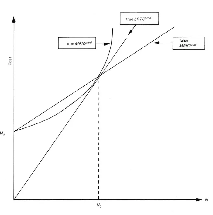
cost context. It will, however, show up as quite important in a marginal cost context. In the diagram of Figure A :2 the systematic downward bias of marginal cost calcula-tions, which is inherent in direct costing, is illustrated by portraying the slopes of the three total cost curves of Figure A : l. The conclusion of the discussion of this appendix can be summarised with reference to the chart in Figure A12.

Of the three curves given there, LRICWOd is the only one which is empirically founded. An estimation of MRICP'Od by statistical methods may prove to be an

over-SMO

FIGURE Al

A diagrammatic representation of the disparaging treatment of the over/leads inherent in direct costing * true LRTCP'Od false od ___-true MR/Cpf + MR/Cprod Co st

Whelming task. In the absence of solid empirical evidence, theoretical reasoning has to be resorted tO. The point made here is that the disparaging treatment ofoverheads inherent in direct costing appears to lead to a systematic underrating of MRlemd. It seems preferable to assume that even the input of overhead factors can be chosen according to normal economic criteria, and thus that MRICD'Od = LRICP'Od under the standard ef ciency conditions.

M.G. PRICING OF SCHEDULED TRANSPORT Jan Owen jansson

FIGURE A2

The resultfor the marginal cost calculation of the disparaging treatment of the overheads

*

Co st true Axon/cmd true]. R/Cp Od I | | | | | | | | | _{falseMR/cefod} | I | | I No REFERENCES

Baumol, W.j., and Vinod, H. D. : An Inventory Theoretical Model of Freight Transport Demand.

Management Science, March 1970.

Borts, G.: The Estimation of Rail Cost Functions. Econometrica, 1960.

Devanney,J. W., III, et al. : Conference Rate-making and the West Coast ofSouth America. Commodity Trans-portation and Economic Development Laboratory, Massachusetts Institute of Technology, 1972.

Ferguson, A. R., et al.: The Economic Value of the United States Merchant Marine. The Transportation Center, Northwestern University, 1961.

Foster, C. D., and Beesley, M. E.: Estimating the Social Bene ts of Constructing an Underground

Railway in London. journal of the Royal Statistical Society, Series A, 126, 1963.

Griliches, Zvi: Cost Allocation in Railway Regulation. The Bell journal of Economics and Management Science, Spring 1972.

Koshal, R. K.: Economies of Scale in Bus Transport: Some Indian Experience. journal of Transport Economics ana' Policy, january 1970.

Koshal, R. K.: Economies Of scale in Bus Transport: Some United States Experience. journal of Transport Economics and Policy, January 1972.

Lee, N., and I. Steedman: Economies of Scale in Bus Transport: Some British Municipal Results.

journal of Transport Economics and Policy, january 1970.

Meyer, j., et al.: T/ze Economics of Competition in the Transportation Industries. Harvard University Press,

1959. »

Mohring, H.: Optimization and Scale Economics in Urban Bus Transportation. American Economic Review, September 1972.

Turvey, R., and H. Mohring: Optimal Bus Fares. journal of Transport Economics and Policy, September 1975.