A T in e p m e th s th b f K J Cent SE-1 Swe
A D
Abstract The aim of th n Sweden. elasticities of performing m main transpo enforced by hat aggregat short-run and hat leisure tr business trav found to be 0 Keywords: A JEL Codes: Ctre for Tra 100 44 Sto eden
emand M
his study is t Using natio f demand are model. The a ort substitute a primitive ted demand d more elasti ravellers, as vellers. Furth 0.44. Aviation, ela C22, D12, Q ansport Stu ockholmModel for D
Fredri CTS Wor to estimate t onal aggrega e estimated w analysis also es to air trav division of for domestic ic (-1.13) in defined in th hermore, the asticity, tran Q58, R41 udiesDomestic
ik Kopsch – rking Papethe price elas ated data on with an unba includes est vel, rail and business and c air travel i the long-run he data, are m cross price nsport, dema
c Air Trav
KTH r 2011:8 sticity of dem n passenger alanced, in te timates of cr d road. The d leisure trav in Sweden is n. The robust more sensiti elasticity be andvel in Swe
mand for dom quantities a erms of statio ross-price ela robustness o vellers. The s fairly elasti tness test of ve to price c etween rail a
eden
mestic air tr and fares, p onarity, yet w asticities for of the result results indi tic (-0.84) in the model sh changes thanand air trave avel price well r the ts is cate n the how n are el is
A Demand Model for Domestic Air Travel in Sweden
Fredrik Kopsch*
KTH – Royal Institute of Technology CTS – Centre for Transport Studies
ABSTRACT
The aim of this study is to estimate the price elasticity of demand for domestic air travel in Sweden. Using national aggregated data on passenger quantities and fares, price elasticities of demand are estimated with an unbalanced, in terms of stationarity, yet well performing model. The analysis also includes estimates of cross-price elasticities for the main transport substitutes to air travel, rail and road. The robustness of the results is enforced by a primitive division of business and leisure travellers. The results indicate that aggregated demand for domestic air travel in Sweden is fairly elastic (-.84) in the short-run and more elastic (-1.13) in the long-run. The robustness test of the model show that leisure travellers, as defined in the data, are more sensitive to price changes than are business travellers. Furthermore, the cross price elasticity between rail and air travel is found to be .44.
JEL classifications: C22, D12, Q58, R41.
Key words: Aviation, elasticity, transport, demand.
*
The author is thankful to Jan-Erik Swärdh, Svante Mandell and Mats Wilhelmsson for valuable input during the process of writing.
1. Introduction
When evaluating the future of the national passenger air transport market it is important to understand what drives demand. For instance, in the light of the forthcoming trade of emission permits for the aviation sector, some new estimates of price elasticities are called for. The demand for air travel has received quite substantial attention in the literature during the past four centuries. The empirical literature contains numerous studies on the determinant of air travel demand. Besides fares, population and income (or GDP where disaggregate data is not available) have been shown to have an impact on air travel demand. 1 However, when studying the price elasticity of short haul flights, i.e. on routes where other modes of transport exists as substitutes to air travel, the price and availability of these will likely be of great importance in determining the demand. For example, if it is relatively cheap to travel by train where air travel is also an option one might expect less people to fly this particular distance. The availability of a substitute to air travel is closely related to the distance of the trip and hence some destinations in Sweden will have more substitutes than others. Of course, the monetary price of other transport modes is not the only factor determining the substitutability of air travel as travel time and other characteristics, such as comfort, play an integral role.
The aim of this study is to, with help of time series analysis, estimate the price elasticity of demand for domestic air travel in the short-, as well as the long-run in Sweden. As a test of robustness of the estimated models, the elasticities for business and leisure travel will be estimated. Control variables for close substitutes, rail and road, will also be included to find cross-price elasticities.
1
This paper is structured as follows, section 2 contains a brief discussion about the demand for air travel, the aim of the following section 3, is to describe and clarify the data used for the analysis. In section 4, the econometrical models used are discussed while section 5 contains a presentation the results. In section 6, the results and their implications are discussed.
2. Literature Review
Jung and Fujii (1976) used a quasi-experiment of cross-sectional city-pair data. The data consisted of travel demand from three cities to a number of destinations during the second quarters of 1972 and 1973. Some of these routes were subject to increases in fares and no city pairs were allowed to differ in schedule frequency. All routes considered in the study were located in the southeast and south central regions of the US with distances ranging between 50 and 500 miles (80 to 800 kilometres). They found that the price elasticity of demand was in the range -1.77 to -3.15.
Straszheim (1978) discusses potential problems with data when estimating the price elasticity of demand for air travel. It is argued that it is hard to separate the effects of changes in price and changes in service provided when using city-pair data over a long period of time as travel demand changes for one destination if other routes become available. The problem can be corrected if the origin and the destination is known for all passengers, it is however very hard to come by data this specific. Another solution is to use aggregated data for the whole market, then all trips by all passengers will be captured. Straszheim used the latter form of data on the north Atlantic region and found evidence of relatively inelastic price elasticity of demand for first class fares, however more elastic than expected. As for economy fares, the price elasticity of demand was found to be elastic and even more so for discounted low fares.
In a related, at least from a geographical point of view, study Fridström and Thune-Larsen (1988) provides estimates of different air transport related elasticities. It was found that the fare elasticity in the short- to medium-run was -.82 while the (undefined) very long-run price elasticity of demand was found to be -1.63. The analysis was performed using link volumes at Norwegian airports, thus resulting in a double counting of passengers transferring flights. This distorting problem was corrected by accounting for the number of transfers at each airport, which is known.
Brons et al. (2002) collected 204 estimates of price elasticities of demand for air travel and conducted a meta-analysis on these previous estimates. One interesting hypothesis in the study was that the price elasticity for Europe ought to be slightly higher than for the US and Australia because of the larger substitutability in passenger travel. This hypothesis was, however, not supported by the data. Among the results it was shown that passengers get more price sensitive over time, i.e. long run elasticities tend to be higher than short-run elasticities. The explanation to this is that it takes time to change behaviour. It is argued that when price elasticities are used for policy implications, the difference between short- and long-run elasticities has to be taken into account.
Anger and Köhler (2010) reviewed several previous studies that had performed estimates of the impact on ticket prices and demand for air travel from the inclusion of the aviation sector into the EU ETS. It is argued that estimates of increases in fares at the higher end, where permit prices in the range of 30-60 euro per tonne have been used, are unlikely to be realised. Furthermore, it is concluded that changes in quantity demanded for air transport will, due to relatively small changes in air fares, be insignificantly small.
3. Data
The data for the analysis stems from several different sources. A national monthly aggregate on departing passengers has been gathered from the Swedish Transport Agency. Unfortunately Origin and Destination (O&D) data for individual passengers have not been available. This essentially means that passengers engaging in one trip with a connecting flight inevitably will be counted twice. To attempt to account for this, a variable describing the share of total passengers in domestic air travel that pass through Arlanda Airport in Stockholm will be included. 2 The logic behind this is simple, if there are fewer direct services between other airports, the number of passengers transferring at Arlanda Airport will increase. The price variable, obtained from Statistics Sweden, is an indexed series of average monthly fares where no distinction is made for different fare categories, e. g. business or leisure travel. In an attempt to distinguish between business and leisure travel, mainly as a test of robustness of the model, a variable explaining price in July will be used. 3 July has traditionally been the month where most Swedes enjoy their vacation, hence it is assumed that business travel is at a minimum during this month and any effect from a price change on demanded quantity would be explained by leisure travellers demand. This will not provide correct point estimates of business and leisure travel but rather a useful illustration of their differences. Furthermore, a similar series, also gathered from Statistics Sweden, of average price of train tickets as well as the cost of driving (an indexed series including price of gasoline) is included. These will account for the two main substitutes to air travel, namely rail and road transportation. A number of economic and demographic variables are included, such as GDP and population size. The data set concerns a time period from January 1980 to
2
Arlanda serves direct routes to all of the Swedish domestic airports, serving as a hub, and an increase in the share of passengers travelling to, or thorugh, Arlanda will serve as a good measurement of direct services between other airports.
3
Combinations of June, July and August have been subject to this study, however, a wider definition of time of vacation will likely include more business travel.
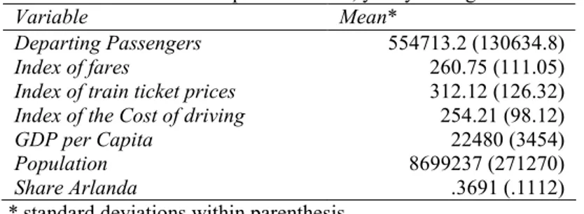
December 2007 and contains 335 observations in total. A brief summery of the most important variables is presented in table I.
Table I. Descriptive statistics, yearly averages
Variable Mean*
Departing Passengers Index of fares
Index of train ticket prices Index of the Cost of driving GDP per Capita Population Share Arlanda 554713.2 (130634.8) 260.75 (111.05) 312.12 (126.32) 254.21 (98.12) 22480 (3454) 8699237 (271270) .3691 (.1112) * standard deviations within parenthesis.
During the 1980’s, the total number of passengers in domestic air travel (shown in Figure I) increased quite dramatically. However, the trend of increasing demand for air travel seems to have been broken in the beginning of the 1990’s. There are numerous reasons that can help explain the decreasing number of passengers in air travel from 1990 and onwards, for example the introduction of high speed rail in 1990, the gulf war and financial crisis and later on, 9/11.
Figure 1: Departing passengers in domestic air travel, Sweden 1980-2007
Departing passengers 0 1000000 2000000 3000000 4000000 5000000 6000000 7000000 8000000 9000000 10000000 1980 1982 1984 1986 1988 1990 1992 1994 1996 1998 2000 2002 2004 2006
Source: Swedish Transport Agency
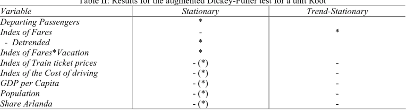
Ideally, all time series used should be integrated of order 0 (I(0)). In other words, they should be stationary. The augmented Dickey-Fuller test for a unit root will help provide evidence of whether or not the time series used are indeed stationary. Results are presented in Table II. All variables but the share of passengers at Arlanda Airport are in logs.
Table II: Results for the augmented Dickey-Fuller test for a unit Root
Variable Stationary Trend-Stationary
Departing Passengers Index of Fares - Detrended
Index of Fares*Vacation Index of Train ticket prices Index of the Cost of driving GDP per Capita Population Share Arlanda * - * * - (*) - (*) - (*) - (*) - (*) * - - - - -
Reject null at 1% significance level, ** Reject the null at 5% significance level, – Falure to reject the null, () First differences. Appropriate variables are in logs.
The two crucial variables are indeed stationary, i.e. integrated of order 0 (I(0)), the number of departing passengers (logged) strictly so while the logged index of fares is stationary allowing for a trend. By applying the Hodrick-Prescott filter the series can be separated into the trend and the detrended series, which is stationary. The null hypothesis of a unit root cannot be rejected for all other variables, hence, these variables are integrated of order 1 (I(1)). They can however be made stationary by differentiation.
4. Model
The demand for any transport mode can be generalized as
(
i k l m)
i f P P x x
z = ... , ... (1)
where zi is the demand for that particular mode of transport (in this case air travel), Pi…Pk are
prices of transport services (own price as well as price of substitutes and complements to the particular transport mode of interest) and xl...xm are other determinants of air travel demand
such as income, population or availability of substitutes. Assuming that other transport modes are substitutes to air travel, which is not far fetched for short haul flights, the cross price elasticity of demand is expected to be positive. Also, the income elasticity is expected to be positive and the own price elasticity is expected to be negative, i.e.,
0 , 0 0 > ∂ ∂ ≠ > ∂ ∂ < ∂ ∂ l i j i i i x z j i P z P z (2)
where Pj is the price of any particular substitute, xl is income and Pi is the price of air fares for
domestic flights. The former relationship is the most interesting for this study but the other ones are also important.
A logged version of the demand function (1) will deliver the wanted elasticities for air travel. Following the specification of demand for air travel made in equation (1) the model can be specified as: t t t t t t t t s Substitute t t t t k t k t t t t t u dummies sharearn population GDPPC P vacation P P P z + + + + + + + + + = − − ) ( ) ( ) ln( ) ln( ) ln( ) * ln( ) ln( ) ln( ) ln( σ ϕ κ γ φ δ β β α (3)
Where Pt is the fare, Pt-k is the lagged effect of fares and Pt * vacation is the variation in price
during vacation, i.e. July. The dummy variables used describe the introduction of high speed rail in 1990 as well as the terror attacks on September 11th, the latter assumes that the effect wore off in 2004. 4 In addition, seasonal dummy variables are included. The primary interest lies in the estimates of βt and βt −k. δt is interesting from a robustness point of view. These three parameters will provide both the short-run (SR) and the long-run (LR) price elasticities for business (sub index B) and leisure (sub index L) of demand for domestic air travel, in particular;
4
∑
∑
− − + + = + = + = = k t t t L k t t B t t L t B LR LR SR SR β δ β β β δ β β (4)Due to multicollinearity in the lagged fare variables individual effects from each lag might show as insignificant. To account for this a simple variable transformation will allow for estimation of the total effect of the lagged fares. This can be illustrated with an example using two lags; ) ln( ) ln( ) ln( ) ln(zt =αt +βt Pt +βt−1 Pt−1 +βt−2 Pt−2 (5) The long-run effect can be defined as the sum of the lags given by;
2 1 − − + + = ≡ t t t LR θ β β β (6)
The total long-run effect can be estimated with;
) ln( ) ln( ) ln( ) ln(zt =αt +θ Pt +βt−1 Pt−1−Pt +βt−2 Pt−2 −Pt (7)
Even if the individual β ’s in (5) show as insignificant due to multicollinearity, the total long-run effect (θ ) in (7) may be significant.
5. Empirical Analysis
A possible problem using a time series model to estimate the price elasticity of demand is that it might be hard to separate effects on the number of departing passengers from price on the one hand, and changes in available services on the other (Straszheim, 1978). During the time period from which data is available, new routes might have been added while other routes have been abandoned. Such changes in service availability that are not necessarily combined with a change in price would most definitely change the number of departing passengers. These disturbances are due to changes on the supply side. As previously discussed, a variable
of the share of all passengers who pass through Arlanda each year is included to account for this.
A Prais-Winsten regression (Prais and Winsten, 1954) is applied to correct for serially correlated error terms that were detected when applying classical linear regression analysis. 5 The regression output is presented in table III.
5
First difference equations have also been estimated with essentially the same results. Output from these are left out and can be found in Appendix A.
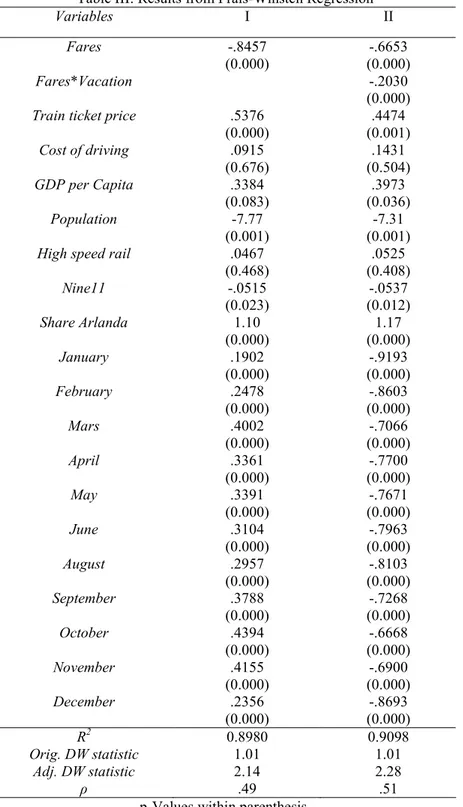
Table III: Results from Prais-Winsten Regression
Variables I II
Fares Fares*Vacation Train ticket price
Cost of driving GDP per Capita
Population High speed rail
Nine11 Share Arlanda January February Mars April May June August September October November December -.8457 (0.000) .5376 (0.000) .0915 (0.676) .3384 (0.083) -7.77 (0.001) .0467 (0.468) -.0515 (0.023) 1.10 (0.000) .1902 (0.000) .2478 (0.000) .4002 (0.000) .3361 (0.000) .3391 (0.000) .3104 (0.000) .2957 (0.000) .3788 (0.000) .4394 (0.000) .4155 (0.000) .2356 (0.000) -.6653 (0.000) -.2030 (0.000) .4474 (0.001) .1431 (0.504) .3973 (0.036) -7.31 (0.001) .0525 (0.408) -.0537 (0.012) 1.17 (0.000) -.9193 (0.000) -.8603 (0.000) -.7066 (0.000) -.7700 (0.000) -.7671 (0.000) -.7963 (0.000) -.8103 (0.000) -.7268 (0.000) -.6668 (0.000) -.6900 (0.000) -.8693 (0.000) R2 Orig. DW statistic Adj. DW statistic ρ 0.8980 1.01 2.14 .49 0.9098 1.01 2.28 .51 p-Values within parenthesis.
Two models are estimated, one with and one without the proxy for leisure travellers. As can be seen the original Durbin-Watson (DW) statistic is far from the wanted value, 2. The adjusted Durbin-Watson statistic suggests that the Prais-Winsten regression successfully corrects for the serial correlation. Aligned with prior expectations the price elasticity decreases when the proxy for leisure travellers is included. Furthermore, as expected, the
cross-price elasticity between air and rail travel is positive, if train ticket prices increase demand for air travel would increase. GDP per capita show a positive and expected coefficient. As mentioned, earlier literature points toward population having a positive effect. This is not the case here, which may be explained by the correlation between GDP per capita and population size. The terrorist attacks on September 11th 2001 show a significant, negative, effect on domestic air travel. Lastly, the proxy for direct flights, the number of passengers passing through Arlanda airport is significantly greater than 0. This result is expected as a greater portion of travellers passing through Arlanda indicates fewer direct services between other airports, thus resulting in a higher number of trips. It is important to keep in mind that the analysis concerns equilibrium points. This essentially means that the price variable used in this analysis is probably endogenously given. In a perfect world, the analysis would model both the demand and the supply sides of the economy. However, it is hard to find sufficient data to allow for modelling of the supply side. Inclusion of a dummy variable describing the deregulation of the domestic air traffic market (from 1992 onwards) shows no result, possibly because of the numerous other factors occurring at the same time (e.g. financial crisis, gulf war, etc.).
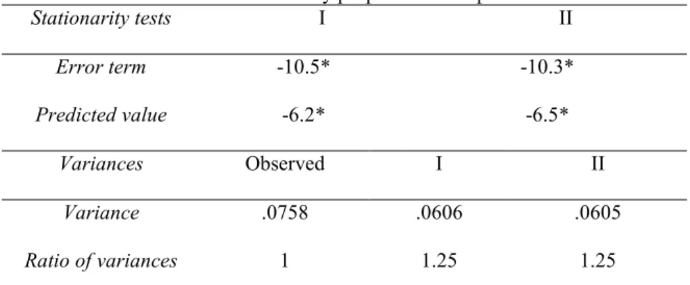
Keep in mind that several of the variables on the right hand side of the equation are I(1) while the dependent variable is I(0) thus resulting in an unbalanced regression. This can potentially lead to biased results and unreliable t-statistics and R2. One way to correct for this is to estimate the model using first differences of the variables, as long as these first differences are I(0).6 However, Pagan and Wickens (1989) state that a minimum criterion for an unbalanced regression is that the error term inherits the stationary property of the dependent variable. Baffes (1997) expands on this and further suggests that if the dependent variable is I(0) and at
6
least two of the independent variables are I(1) the model can still be considered well performing if the predicted value of the dependent variable is also I(0) and the variance of the observed and predicted dependent variable are equal. This proposes three criteria for the model to fulfil.
Table IV: Tests of stationary properties and equal variances. Stationarity tests I II Error term Predicted value -10.5* -6.2* -10.3* -6.5* Variances Observed I II Variance Ratio of variances .0758 1 .0606 1.25 .0605 1.25
In our stationarity tests * denotes rejection of the null of an existing unit root at the 1 percent significance level.
The test results, as seen in table IV, are somewhat ambiguous. On the one hand, the error term has inherited the stationary properties of the dependent variable suggesting that the model is well behaved. The stationary properties of the predicted values that each model produce, point towards the same conclusion. In all cases, the null of equal variances can be rejected, i.e. the ratios are significantly different from 1, however, not far from 1. The critical F-statistical values are 1.2 which suggests that the models come very close. These tests indicate that the models are reliable.
Now short-run, or immediate, price elasticities of demand for both business and leisure travel in Sweden have been successfully estimated. In order to assess the long-run effect, an optimal number of lags need to be included in the model. From the Schwarz’s and Bayesian Information Criterion (SBIC) the optimal number of lags is six.7
7
Akaike’s Information Criterion and the Hannan Quinn Information Criterion suggest 8 and 7 lags respectively. However, the point estimates do not vary significantly in comparison to 6 lags. 6 months does however seem like a reasonable time frame.
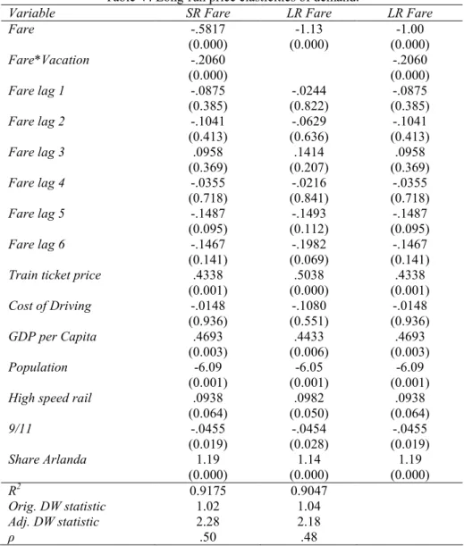
Table V: Long-run price elasticities of demand.
Variable SR Fare LR Fare LR Fare Fare Fare*Vacation Fare lag 1 Fare lag 2 Fare lag 3 Fare lag 4 Fare lag 5 Fare lag 6 Train ticket price Cost of Driving GDP per Capita Population High speed rail 9/11 Share Arlanda -.5817 (0.000) -.2060 (0.000) -.0875 (0.385) -.1041 (0.413) .0958 (0.369) -.0355 (0.718) -.1487 (0.095) -.1467 (0.141) .4338 (0.001) -.0148 (0.936) .4693 (0.003) -6.09 (0.001) .0938 (0.064) -.0455 (0.019) 1.19 (0.000) -1.13 (0.000) -.0244 (0.822) -.0629 (0.636) .1414 (0.207) -.0216 (0.841) -.1493 (0.112) -.1982 (0.069) .5038 (0.000) -.1080 (0.551) .4433 (0.006) -6.05 (0.001) .0982 (0.050) -.0454 (0.028) 1.14 (0.000) -1.00 (0.000) -.2060 (0.000) -.0875 (0.385) -.1041 (0.413) .0958 (0.369) -.0355 (0.718) -.1487 (0.095) -.1467 (0.141) .4338 (0.001) -.0148 (0.936) .4693 (0.003) -6.09 (0.001) .0938 (0.064) -.0455 (0.019) 1.19 (0.000) R2 Orig. DW statistic Adj. DW statistic ρ 0.9175 1.02 2.28 .50 0.9047 1.04 2.18 .48 p-Values within parenthesis.
Since there is strong multicollinearity between the lagged price variables, the variable transformation from (7) is used to estimate the summed long-run effect of a permanent price change. The regression output from the long-run estimates, as seen in table V, point towards higher elasticities in the long-run than in the short-run. As discussed, this is an expected result. Other than that, all other point estimates are close to what they were in the static model. 8 The same three test criteria for an unbalanced regression are applied. The results
8
The model is still corrected for seasonal changes in departing passengers but this is left out from the table. Estimates and p-values are the same as before.
point towards the same direction as earlier, the ratio of variances is, however, slightly higher at 1.41.
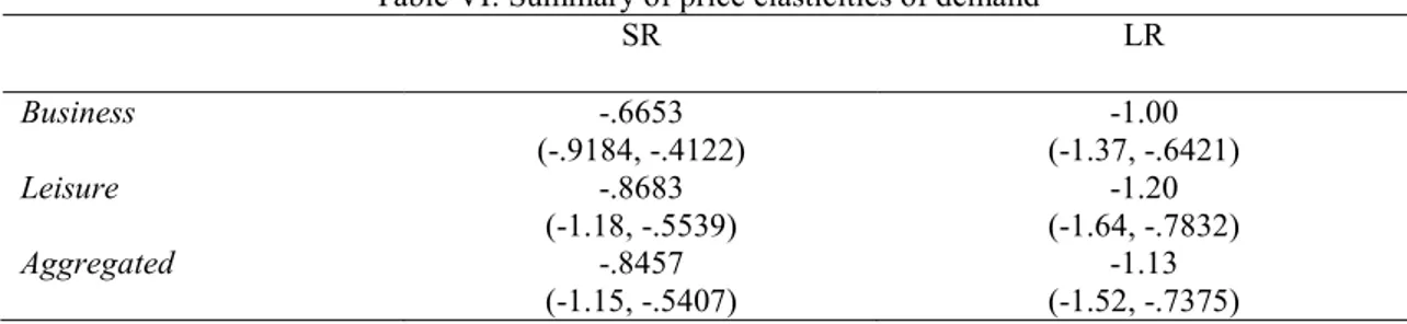
Table VI: Summary of price elasticities of demand
SR LR Business -.6653 (-.9184, -.4122) -1.00 (-1.37, -.6421) Leisure -.8683 (-1.18, -.5539) -1.20 (-1.64, -.7832) Aggregated -.8457 (-1.15, -.5407) -1.13 (-1.52, -.7375)
A summary of the estimated price elasticities of demand for domestic air travel for both business and leisure passengers in the short- and the long-run is presented in table VI (confidence intervals within parenthesis), an aggregated estimate is also provided. Noteworthy is that the short-run elasticity for business is statistically different from -1, suggesting that the Swedish market for business air travel is indeed price insensitive.
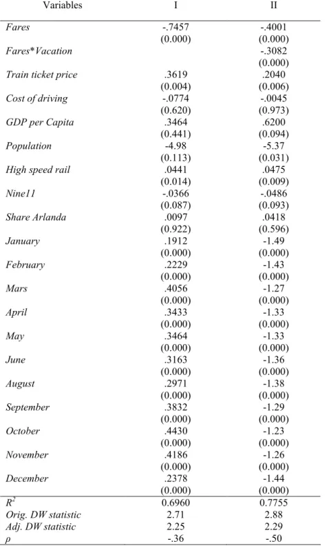
The approach to handling unbalanced regressions with many non-stationary variables used in this paper is unconventional and has not been substantially tested in the literature. A more conventional approach to handling non-stationarity is to use a first-difference model. In addition to the model presented in this paper one such first-difference model has also been estimated. The results from this estimation can be seen in appendix A. Over all, the results from the first difference approach differ from the earlier results by 1 or 2 decimal points. The point estimates for the aggregated travel demand as well as for leisure from the first difference model both fall within the confidence intervals of the earlier results. The first difference point estimate for business falls just outside of the corresponding confidence interval. These results further strengthen the analysis provided in this paper.
6. Concluding remarks
The aim of this study was to estimate the price elasticity of demand for domestic air travel in both the short- and the long-run in Sweden. In order to do this, a time series model was constructed. The individual effects of increases in fares on business and leisure travel were estimated by including a price variable for the month of July, when Swedes traditionally enjoy their vacation. While this method does not give exact point estimates it provides useful evidence to the difference between the two travel groups. The specific choice of July as the month of vacation can be questioned. Combinations of the months June, July and August can also act as good proxies for vacation time but a wider definition of the time for vacation will likely also include more business travellers resulting in less distinguished estimates. The findings of this study correspond to what earlier studies have concluded. 9 Two general finding is that the fare elasticity is larger (in absolute numbers) for leisure than for business travellers and also that the fare elasticity in the long-run is larger (in absolute numbers) than in the short-run. Fridström and Thune-Larsen’s (1988) estimates for Norway provide a good base for comparison of the point estimates because of the similar estimation method as well as similar geographical characteristics as Sweden. They provide an aggregate short-run direct fare elasticity of -.82, very close to the aggregated fare elasticity of -.84 presented in this paper. The aggregated long-run fare elasticity of -1.13 presented in this paper is lower (in absolute numbers) than the very long-run fare elasticity presented by Fridström and Thune-Larsen. The long-run results from this study might not be comparable to the ones presented by Fridström and Thune-Larsen since different time horizons might have been used. Furthermore, the cross price elasticity for train, one of the closest substitutes to domestic air travel in Sweden came out positive.
9
There are some exisiting evidence of fare elasticity in Sweden from before. The are in the range -.1 to -1.13 and -.2 to -1.0 for business and leisure travel respectively. For more information see for example SIKA Rapport 2002:19 or SIKA PM 2006:2 (both in Swedish).
References
Anger, A., J. Köhler (2010). ‘Including aviation emissions in the EU ETS: Much ado about nothing? A review’, Transport Policy 17 (2010), 38-46.
Ba-Fail, A. O., S. Y. Abed, S. M. Jasimuddin (2000). ‘The Determinants of Domestic Air Travel Demand in the Kingdom of Saudi Arabia’, Journal of Air Transportation World Wide, Volume 5, No. 2, 72-86.
Baffes, J. (1997). ’Explaining stationary variables with non-stationary regressors’, Applied Economics Letters 4:1, 69-75.
Brons, M., E. Pels, P. Nijkamp, P. Rietveld (2002). ’Price elasticities of demand for passenger air travel: a meta-analysis’. Journal of Air Transport Management 8, 165-175.
Fridström, L. Thune-Larsen, H. (1989). ‘An econometric air travel demand model for the entire conventional domestic network: The case of Norway’. Transportation Research Part B Volume 23B No.3, 213-223.
Ito, H. Lee, D. (2004). ’Assessing the impact of the September 11 terrorist attacks on the U.S. airline demand’. Journal of Economics and Business 57, 75-95.
Jung, J.M., Fujii, E.T. (1976). ’The Price Elasticity of Demand for Air Travel – Some New Evidence’, Journal of Transport and Policy Economics and Policy 10, 257-262.
Mason, K. J., (2005). ‘Observations of fundamental changes in the demand for aviation services’. Journal of Air Transport Management 11 (2005), 19-25.
Pagan, A. R., and M. R. Wickens (1989). ‘A survey of some recent econometric methods’, Economic Journal 99, 962-1025.
Prais, S. J., and C. B. Winsten (1954). ‘Trend estimators and serial correlation’, Cowles Commission Discussion Paper No. 383, Chicago.
Sika Rapport 2002:19 (2002). ‘Metoder och riktlinjer för bättre samhällsekonomiskt beslutsunderlag’, Delrapport ASEK, Stockholm.
Straszheim, M.R. (1978). ‘Airline Demand Functions in The North Atlantic and Their Pricing Implications’, Journal Transport Economics and Policy 12, 179-195.
Wit, R.C.N, B.H. Boon, A. van Velzen, M. Cames, O. Deuber, D.S. Lee, (2005). ‘Giving wings to emissions trading – Inclusion of aviation under the European emissions trading system (ETS): design and impacts’. Report for the European Commission, DG Environment.
APPENDIX A
In contrast to the unbalanced regression, an estimation where all variables are integrated of the same order, specifically I(0), would be interesting to see. In order to achieve this, the first difference approach will be used, i.e. all variables are in differences. Again some first order serial correlation is detected in the error term and hence the Prais-Winsten regression is used to correct for this.
Table V: Results from first difference Prais-Winsten Regression
Variables I II
Fares
Fares*Vacation Train ticket price Cost of driving GDP per Capita Population High speed rail Nine11 Share Arlanda January February Mars April May June August September October November December -.7457 (0.000) .3619 (0.004) -.0774 (0.620) .3464 (0.441) -4.98 (0.113) .0441 (0.014) -.0366 (0.087) .0097 (0.922) .1912 (0.000) .2229 (0.000) .4056 (0.000) .3433 (0.000) .3464 (0.000) .3163 (0.000) .2971 (0.000) .3832 (0.000) .4430 (0.000) .4186 (0.000) .2378 (0.000) -.4001 (0.000) -.3082 (0.000) .2040 (0.006) -.0045 (0.973) .6200 (0.094) -5.37 (0.031) .0475 (0.009) -.0486 (0.093) .0418 (0.596) -1.49 (0.000) -1.43 (0.000) -1.27 (0.000) -1.33 (0.000) -1.33 (0.000) -1.36 (0.000) -1.38 (0.000) -1.29 (0.000) -1.23 (0.000) -1.26 (0.000) -1.44 (0.000) R2 Orig. DW statistic Adj. DW statistic ρ 0.6960 2.71 2.25 -.36 0.7755 2.88 2.29 -.50 p-Values within parenthesis.