Journal for Person-Oriented Research
2016, 2(3), 142-154Published by the Scandinavian Society for Person-Oriented Research Freely available at http://www.person-research.org
DOI: 10.17505/jpor.2016.14
142
Using local linear models to capture dynamic interactions
between cortisol and negative affect
Roelof B. Toonen, Klaas J. Wardenaar, Sanne H. Booij, Elisabeth H. Bos, & Peter de Jonge
University of Groningen, University Medical Center Groningen, Interdisciplinary Center Psychopathology and Emotion Regulation, Groningen, The NetherlandsCorresponding author:
Roelof B. Toonen, Interdisciplinary Center Psychopathology and Emotion Regulation, CC72, University Medical Center Groningen, University of Groningen, Hanzeplein 1, 9700 RB Groningen, the Netherlands
Email: r.b.toonen@umcg.nl
To cite this article:
Toonen, R. B., Wardenaar, K. J., Booij, S. H.., Bos, E. H., & de Jonge, P. (2016), Using local linear models to capture dynamic interactions between cortisol and negative affect. Journal for Person-Oriented Research, 2(3), 142-154. DOI:
10.17505/jpor.2016.14.
Abstract
Objective: Previous studies have found both increased and decreased cortisol levels in depressed patients. These inconsistent
findings may be explained by the fact that traditional group-based studies are not suitable to capture complex intra-individual dynamics between cortisol and affect, and inter-individual differences therein. The current study used a time-series approach to gain deeper insight into the nature of these complex dynamics and to investigate possible underlying nonlinear dynamical features.
Method: Time-series data (90 measurements) were collected for cortisol and negative affect (NA) in depressed (n=15) and
non-depressed (n=15) participants. The relationship between cortisol and NA in each individual was analyzed with SMAP, which estimates local linear vector autoregression (VAR) models with different degrees of nonlinearity in the prediction. The best-predicting model, and whether this model was linear or nonlinear, was determined by using the normalized root mean square error (NRMSE) between the models’ predicted values and the observed values. Univariate and multivariate models were compared to explore the connection between cortisol and NA.
Results: Nonlinear cortisol predictions were best in 90% of the participants, whereas nonlinear NA predictions were best in
39% of the participants. Multivariate analyses showed that in 48% of the participants, cortisol was better predicted when NA was included in models that otherwise consisted of time delayed values of cortisol alone. Vice versa, in 39% of the partici-pants, NA was better predicted when cortisol was included in models that otherwise consisted of time delayed values of NA alone. The connection between cortisol and NA was stronger in the depressed group, although the results showed consider-able inter-individual heterogeneity within the diagnostic groups.
Conclusion: In many individuals, cortisol and NA may be interacting parts of a common dynamical system and their
con-nection may be stronger in depressed patients.
143
Introduction
Disturbances in the hypothalamic-pituitary-adrenal (HPA) axis have been among the most widely studied etiological pathways in depression (Pariante & Lightman, 2008). However, the precise nature of the relationship between the hormones secreted by the HPA axis (e.g. cortisol, adrenocorticotropic hormone [ACTH], and cor-ticotropin releasing hormone [CRH]) and depression is still unknown (Stetler & Miller, 2011). Several studies observed increased levels of the stress hormone cortisol in depressed patients compared to healthy controls (Bhagwagar, Hafizi, & Cowen, 2005; Vreeburg et al., 2009). However, other studies showed decreased cortisol levels in depressed patients or found no difference in cortisol levels at all (e.g. Stetler & Miller, 2005; Huber, Issa, Schik, & Wolf, 2006). These inconsistencies could have been caused by a number of factors, such as differ-ing study designs/procedures and the heterogeneity of the depression phenotype.
Another important reason could lie in the fact that previous findings have been mostly derived from cross-sectional studies that assessed cortisol only a sin-gle time or a few times per day within subjects. By tak-ing this approach, the highly dynamic nature of cortisol, depression and their causal relationship over time is ne-glected (e.g. Booij et al., 2015). It is questionable whether cross-sectional associations that are found at the inter-individual level (e.g. group differences) are gener-alizable to the intra-individual level, that is: temporal relationships between factors within the person (Mo-lenaar & Campbell, 2009). Unfortunately, studies that have investigated intra-individual relationships are scarce, leaving it unclear how changes in cortisol and depressive symptomatology are related within persons. Changes in cortisol could cause changes in sympto-matology and/or vice versa.
To capture the dynamic intra-individual relationship between cortisol and depressive symptomatology, a time-series approach may be more adequate than group-based approaches. A hallmark of intensive time-series designs is the use of many repeated meas-urements within a single person. A study by Booij, Bos, de Jonge, and Oldehinkel (2016) analyzed the relation-ship between cortisol and negative affect using a linear time-series approach. They found a considerable amount of heterogeneity between participants in the way that daily life fluctuations in cortisol are related to affective states. The time-series analysis methods that were used in this study are designed to find linear relationships between variables (Prado and West, 2010). When the objective of these linear analyses is to answer questions about causal relationships, time-series-based methods like inferences for Granger Causality (GC) can be ap-plied (Granger, 1988).
However, many systems in nature are complex, mak-ing it likely that the relationships between the variables of interest are complex and nonlinear. Mathematically, linear relationships between two or more variables take the form
y = c
1x
1+ c
2x
2+ ···
. Nonlinear relationshipstake more complex forms, for instance
y = c
1x
1(x
1+ c
2x
2) + ···
, where the influence of onevariable (
x
1) depends on the value of another variable(
x
2). These relationships can usually not be captured bylinear models. Consequently, causality inferences with GC may not be able to detect the nonlinear causal con-nections that exist between variables (Sugihara et al., 2012). In these cases, nonlinear analytical approaches that are based on dynamical systems theory may be preferable (Kantz & Schreiber, 2004).
Several nonlinear approaches to time-series analysis are available. A particular class of nonlinear models ap-ply local linear approximation techniques to predict val-ues of a variable (Farmer & Sidorowich, 1987; Sugihara, 1994; Casdagli, 1989). Typical for these techniques is that time-series data are transformed into an embedding. This is a collection of points (vectors) in a coordinate space, with each point corresponding to a point in the time-series data. The coordinates of each point are de-termined by taking a value in the time series at a time t, together with past values of the series, separated by equidistant time intervals. Although time is not a dimen-sion in the resulting space, the embedding still represents the dynamics of the system. Instead of following a time series along a t-axis, progression in time now follows a line through connected points in the embedding. A set of points around a target point may now be used to con-struct a linear model which can be applied to the target point to predict an associated value (e.g. a future value of the same variable, or a value in the time series of an-other variable). This procedure results in a unique local linear model for each target point, allowing for the esti-mation of nonlinear relationships. By varying the num-ber of used neighbor points in the prediction, or by var-ying the weight of the neighbor points (i.e. a stronger weight to close neighbors than to distant neighbors), the extent of local operation can be controlled.
This approach is different from traditional global lin-ear techniques, where all values are used to estimate a joint model for all data points. Furthermore, by measur-ing the extent of local operation that is needed to obtain the best prediction results, insight into the nonlinearity of the underlying system is obtained. In nonlinear sys-tems, global predictors will show a lower prediction performance compared to local predictors. In linear sys-tems, global predictors will show better performance than local predictors (Sugihara, 1994).
Several methods exist to select neighborhood points for the local models. In one approach (as used by Farmer & Sidorowich, 1987), only k nearest neighbors of the
144
target are selected, with k being an adjustable constant. In another approach, only neighbors within a certain distance from the target are used (Kantz & Schreiber, 2004). Finally, an elegant and flexible way of selecting neighborhood points is obtained by applying a weight
function
w(d) = exp(-θd/d
avg)
to each point in thecomplete data set before feeding the vectors and pre-dictees into the linear prediction model. Here d is the distance between the predictee and the neighbor, θ the nonlinearity parameter controlling the width of the
func-tion, and
d
avg the average distance between the predicteeand all other vectors within the embedding. This ap-proach is called the SMAP method and was introduced by Sugihara (1994) (see Figure 1). The weight function assigns greater weight to points closer to the predictee, corresponding to a bigger influence on the fitted linear model. By varying the width of the weight function, it is possible to fit a range of models, varying from extremely local to completely global, the latter of which would be comparable to regular vector autoregressive (VAR) modeling (Brandt & Williams, 2007).
In this study, the SMAP procedure was used in com-bination with a VAR model. The VAR parameters were computed with a total least squares (TLS) procedure based on singular value decomposition (Van Huffel & Vandewalle, 1991). In TLS fitted models, uncertainty is assumed in the dependent variable and in the independ-ent variables. Ordinary least squares fitted models as-sume uncertainty in the dependent variable only (Golub and van Loan, 1980). In diary studies, uncertainty can often be assumed in both variables. Therefore a TLS-fitted model will better reflect the uncertainty that is present in the data.
The aim of the current study was to investigate the usefulness of SMAP for applied psychophysiological research. SMAP was used to study the nature of the in-tra-individual relationship between cortisol and negative affect (NA) (an important symptom domain of depres-sion), using time-series data that were collected three times per day for 30 days in 15 participants with a Major Depressive Disorder (MDD) and in 15 pair-matched non-depressed participants. For each participant, the extent of nonlinearity in his/her time series was investi-gated by comparing prediction of local and global mod-els. Also, the direction of the relationship between corti-sol and NA was investigated. Finally, the results ob-tained in the individual participants were summarized to investigate the extent of variation in (non)linearity and directionality of the relationship across participants, and between the depressed and non-depressed groups.
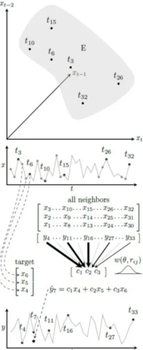
Figure 1. Univariate SMAP illustrated.
An embedding (E) is created by extracting lagged vectors from time-series data for x. This is illustrated for a target vector at t = 6, having scalar components that are obtained by taking the value of
x at t = 6, t = 5 and at t = 4. A prediction ( ) for the future value
of an associated variable y (which may be x itself) at t = 7, is ob-tained as the outcome of a linear vector regression on the target vector’s components. The parameters (c1,c2,c3) of this regression
are estimated from the relationship between the target’s neighbors (i.e. all other vectors in the embedding) and their associated val-ues of y. A gaussian weight function w, depending on the tar-get-neighbor distance rij, determines the influence of a neighbor
on the values of the parameters, with closer neighbors having more influence than distant ones. The width (or flatness) of this gaussian curve is controlled by θ. Individual models are estab-lished for each vector of the embedding.
145
Method
Participants
Data were obtained from the MOOVD study (Bouwmans et al., 2015). This dataset contains time-series data (three measurements per day, 30 con-secutive days, 90 measurements in total) for several bi-ological markers, various diary items, and movement variables. Data were collected in 54 individuals, of whom 27 had an MDD (currently or in the past 2 months) and 27 were non-depressed. Patients and healthy sub-jects were matched on sex, age, body mass index and smoking status. For the analyses of the present study a subset of 30 participants (age 20 to 50 years) was used, i.e. those for whom cortisol measurements were availa-ble. The selection consisted of 15 participants with a major depressive disorder (MDD) (ID 1 to 15) and 15 non-depressed participants (ID 16 to 30). The study pro-tocol was approved by the Medical Ethical Committee of the University Medical Center Groningen (UMCG). All participants provided written informed consent.
Ambulatory sampling
A PsyMate device (PsyMate BV, Maastricht, The Netherlands) (Myin-Germeys, Birchwood, & Kwapil, 2011) was used to administer an electronic questionnaire to the participants. Three times a day, at 10 AM, 4 PM, and 10 PM (on average; the sampling scheme was ad-justed to the participant’s sleep-wake schedule), the par-ticipants were warned with an acoustic signal to fill out the questionnaire, which consisted of 60 items relating to mood, activity, and cognition. The duration of the total diary study was 32 days, of which the first two days were used for the participants to get used to the proce-dure and the following days were used for data collec-tion. This resulted in up to 90 measurements per partici-pant. The average number of missing cortisol values per participant was 4.2 (s.d. = 4.2) and the average number of missing NA values per participant was 6.5 (s.d. = 6.0).
Cortisol
The participants used Salivettes®; to collect saliva samples while they filled out the electronic diary and stored these samples in their home refrigerator until they were collected by research staff (once per week). After collection, the samples were centrifuged and stored in the UMCG laboratory, at -80 °C. Online-solid phase extraction in combination with isotope dilution liquid chromatography-tandem mass spectrometry was applied to 250 µL of saliva, using deuterated cortisol as internal standard. All samples of one participant were processed
in the same batch. Mean intra- and inter-assay coeffi-cients of variation were below 10%. The quantification limit for cortisol was 0.1 nmol L-1.
Negative affect
A NA score was obtained by computing the average of the mood items ’tense’, ’anxious’, ’distracted’, ’rest-less’, ’irritated’, ’depressed’, and ’guilty’ from the diary data. These items were adapted from Bylsma, Tay-lor-Clift, and Rottenberg (2011) and were rated on a 7-point Likert response scale (range: 1 = ’not’ - 7 = ’very’).
Data preparation
First-differences of time series for cortisol and NA were taken to remove linear trends from the series with-out compromising the possible nonlinear nature of the data. The first-differenced time series were scaled to zero mean and unit variance.
Embedding construction and validation
To construct the univariate embeddings, lagged vec-tors Vt = [xt, xt-1,…, xt-(e-1)] (where e is the dimension of
the embedding), were constructed from the time-series data of either cortisol or NA. Vectors containing missing values were omitted from inclusion. Each vector was associated with a predictee; that is: a future value of the same variable or a future or contemporaneous value of the other variable. Given the limited amount of observa-tions, leave-one-out validation was used when compu-ting the prediction performance (Arlot, Celisse, et al., 2010). The multivariate embeddings were constructed by taking the best performing univariate embedding and adding values from the time series of the other variable (Cao, Mees, & Judd, 1998). In the current study, only one lag of the other variable was used. Using two or more lags resulted in too much data loss because of omission of the vectors with missing values. The com-bination of vectors and predictees was used to construct (local) linear models and to validate predictions made by applying these models to target vectors (which were ex-cluded in the model creation step).
Cortisol predictions
To test the prediction of cortisol by NA, two types of embedding were constructed: a univariate cortisol em-bedding to test for the ability of cortisol to predict future values of itself and a multivariate embedding consisting of cortisol and NA to test for the amount of improve-ment in predictive ability if NA was added to the cortisol embedding. For each type of embedding, a range of di-mensions was produced: for the univariate case with dimension 1, an embedding was constructed consisting
146
of cortisol values with lag 1, to predict the cortisol value at time t. For dimension 2 the values of lag 1 and lag 2 were used to predict the value at time t. For dimension 3 the values of lags 1, 2 and 3 were used, and so on. Em-bedding dimensions of up to 7 were used. The multivari-ate embeddings were constructed by taking the univari-ate embeddings and adding values from one lag of NA. This lag was taken from a range of lag 0 (i.e. the con-temporaneous value of the cortisol predictee) to lag 4. For each embedding, the nonlinearity parameter θ was varied between 0.0 and 3.0 in steps of 0.2. The predic-tive performance of an embedding was assessed at each value of θ by computing the normalized root mean square error (NRMSE) between the predicted and ob-served values of cortisol. To obtain the NRMSE, the root mean square error (RMSE) between the observed and predicted values was divided by the standard deviation of the observations that were used in the embedding. Due to cortisol’s natural fluctuation pattern during the day (Stone et al., 2001), showing high levels in the morning and a gradual decay over the rest of the day, the standard deviation of the observations will typically be higher than the RMSE of the observed and predicted values, resulting in a low NRMSE. This may obscure the real prediction performance of the method. Therefore, the NRMSE was also computed separately for the values collected in the morning, the afternoon, and the evening.
Negative affect predictions
Similar to the cortisol predictions, NA was predicted using univariate and multivariate embeddings, consisting of NA predicting NA and of NA plus cortisol predicting NA, respectively. Embedding parameters were varied in the same way as was done for the cortisol predictions. Here again θ was varied between 0.0 to 3.0 in steps of 0.2 and the NRMSE was calculated at several, increas-ing values of θ.
Bootstrapping and testing
A bootstrapping procedure was applied to obtain es-timates for the distribution of the computed NRMSE’s. In each bootstrap, a new embedding was constructed by sampling points from the original embedding, thus re-sembling an overlapping blocks bootstrap procedure with blocks that contain the scalar components of one vector each (Härdle, Horowitz & Kreiss, 2003). The sampling procedure was constructed in such a way that the bootstrapped embeddings would contain the same number of morning, afternoon, and evening values as the original embedding. For each combination of lags and
variables, 1000 bootstrap embeddings were used, result-ing in 1000 separate estimates for the NRMSE at each value of θ. Subsequently, an average was computed at each value of θ for each embedding. These averages were computed for the full embedding and for the sepa-rate time-of-day predictions. This resulted in prediction graphs as shown in Fig. 2. Based on these averaged pre-dictions, the best-performing model with optimal bedding parameters was identified by choosing the em-bedding and parameter θ that resulted in the lowest av-erage NRMSE.
A Mann-Whitney test (Altman, 1990) was used to test for the significance of the difference between the NRMSE distribution at the optimal value of θ and the NRMSE distribution at θ = 0 (global/linear prediction). The same testing approach was used to test the differ-ence between the NRMSE distributions obtained from univariate and multivariate embeddings.
Software
Software to construct the embeddings, generate boot-strap sets, and compute prediction performance was programmed in C on linux. This software is available upon request. Total least square fitting routines devel-oped by Van Huffel and Vandewalle (1991) were used to obtain linear model fits. Additional analyses were car-ried out in R (R Core Team, 2015).
Results
Prediction of cortisol with and without
nega-tive affect
The NRMSE for the univariate cortisol embeddings
(Table 1) showed significantly lower values for the local linear models in comparison with the global linear
mod-els, with Δnrmselin values greater than zero in 27 out of
30 participants (90%). Here, Δnrmselin represents the
difference between the NRMSE in the global linear em-bedding (θ = 0) and the NRMSE in the optimal embed-ding. These values were based upon results from the complete embedding, without distinguishing between different times of day. Separate predictions for each time of day showed better local prediction performance for the morning values in 26 out of 30 participants (87%), for the afternoon values in 25 out of 30 participants (83%) and for the evening values in 16 out of 30 partic-ipants (53%).
147 Figure 2: Results of SMAP for participant 23.
SMAP predictions are shown for two analyses: cortisol predictions based upon a univariate cortisol embedding (Cortisol), and cortisol predictions based upon a multivariate cortisol + negative affect embedding (Cortisol + NA). Results have been obtained for: all time series values, and for the morning, afternoon and evening values separately. Each panel shows the results for several embeddings, each having different embedding parameters. The multivariate results were obtained by taking the best performing univariate embedding and adding one lag of NA at various values for the distance of this lag. Values for the NRMSE have been obtained as an average of 1000 bootstrap runs. Parameter θ ranges from 0 (completely global) to 3 (extremely local).
148
Table 1
Performance of cortisol predictions.
ID cortisol cortisol negaff
dim n nrmse ∆nrmselin θ dim n nrmse ∆nrmselin θ lagNA Impr Imprlin
1 2 55 0.437 0.020*12 1.40 3 34 0.445 0.007* 23 0.60 6 -0.008 123 0.011 2 2 63 0.463 0.137*123 1.60 3 55 0.528 0.113*123 1.40 3 -0.065 0.043 3 2 75 0.362 0.044*12 1.40 3 69 0.346 0.082*123 1.80 3 0.016*1 3 0.006 4 2 61 0.708 0.000 2 0.00 3 46 0.654 0.000 0.00 7 0.054*123 0.054 5 2 67 0.489 0.044*123 1.00 3 63 0.460 0.044*123 1.40 3 0.029*1 0.030 6 2 66 0.679 0.027*12 0.80 3 63 0.653 0.022*123 0.80 2 0.026*1 0.034 7 2 60 0.552 0.000 2 0.20 3 51 0.448 0.050*123 1.00 0 0.104*12 0.054 8 2 71 0.419 0.070*123 1.40 3 48 0.399 0.017*123 1.60 1 0.020*123 0.073 9 2 67 0.559 0.041*1 1.20 3 55 0.568 0.029*1 1.20 4 -0.009 23 0.005 10 2 69 0.496 0.018*123 0.80 3 61 0.479 0.004 23 0.40 3 0.017*1 0.030 11 2 71 0.483 0.124*123 1.40 3 64 0.515 0.115*123 1.60 3 -0.032 -0.014 12 1 74 0.998 0.014*12 0.20 2 48 0.943 0.025*12 0.20 4 0.055* 23 0.045 13 2 71 0.516 0.078*123 1.40 3 66 0.526 0.021*123 1.00 5 -0.010 1 3 0.048 14 2 79 0.594 0.040*123 1.00 3 74 0.592 0.032*123 0.80 5 0.002 0.009 15 2 77 0.417 0.052*123 1.20 3 77 0.417 0.058*123 1.80 1 -0.000 1 0.008 16 2 35 0.726 0.008 0.40 3 27 0.760 0.000 0.00 6 -0.034 -0.026 17 2 61 0.527 0.127*123 1.20 3 56 0.522 0.073*123 1.20 7 0.005*12 0.058 18 2 71 0.383 0.010* 23 1.00 3 60 0.369 0.000 0.00 7 0.014* 3 0.025 19 2 56 0.633 0.038*123 1.00 3 45 0.608 0.002 23 0.20 5 0.025*123 0.061 20 3 58 0.410 0.204*123 0.80 4 54 0.406 0.132*123 0.80 3 0.004* 2 NA 21 2 65 0.710 0.082*123 1.00 3 59 0.740 0.053*123 1.20 5 -0.030 -0.001 22 2 68 0.278 0.020*1 3 1.20 3 57 0.273 0.005 3 1.00 2 0.005*1 3 0.022 23 2 40 0.783 0.075*123 0.60 3 30 0.815 0.094*123 1.00 5 -0.032 23 -0.051 24 2 63 0.397 0.030*12 1.20 NA NA NA 25 2 75 0.354 0.005*12 0.80 3 72 0.366 0.001 2 0.20 5 -0.012 123 -0.008 26 2 38 0.410 0.023*12 1.20 3 27 0.321 0.015*1 3 0.80 4 0.089*123 0.097 27 2 72 0.368 0.012*123 1.20 3 70 0.370 0.002 3 0.40 4 -0.002 0.007 28 2 53 0.539 0.048*12 1.20 3 47 0.586 0.031*12 0.80 1 -0.047 -0.030 29 2 61 0.443 0.008*12 0.80 3 55 0.478 0.000 0.00 2 -0.035 1 -0.028 30 2 77 0.353 0.008*12 1.20 3 68 0.370 0.006* 2 0.40 1 -0.017 -0.016
* p < 0.05 for the indicated difference, based on the complete embedding. 1,2,3 p < 0.05 for the corresponding morning, afternoon, or
evening differences respectively. ID 1 through 15: depressed participants; ID 16 through 30: non-depressed participants.
Note. Performance of cortisol predictions for multivariate embeddings consisting of cortisol and negative affect (NA), and univariate embeddings consisting of cortisol only. The values shown are the values that were obtained from the complete embedding, without dif-ferentiating between time of days. For each participant, the following parameters are shown: dim, the dimension; n, the number of time series points used; nrmse, the normalized root mean square error between the predicted values and the observed values; ∆nrmselin, the
difference between the optimal NRMSE and the NRMSE for the global linear case (with θ = 0), with positive values indicating a better performance for the local linear predictions; lagNA, the negative affect lag which – when added to the optimal embedding – results in the lowest NRMSE; Impr, the difference between the NRMSE of the multivariate embedding and the NRMSE of the univariate embedding;
Imprlin, The difference between the NRMSE of the multivariate embedding and the NRMSE of the univariate embedding when only
149
Table 2.
Performance of negative affect predictions.
ID negaff negaff cortisol
dim n nrmse ∆nrmselin θ dim n nrmse ∆nrmselin θ lagCo Impr Imprlin
1 1 51 1.071 0.048*12 0.20 2 46 1.542 0.019 1 0.20 1 -0.471 1 -0.443 2 1 73 1.135 0.000 0.00 2 66 1.105 0.006*1 3 0.20 1 0.030* 2 0.024 3 2 78 0.742 0.039*1 3 0.80 3 72 0.665 0.036* 23 0.60 1 0.077*1 3 0.080 4 1 71 1.173 0.000 0.00 2 65 1.453 0.000 1 0.00 0 -0.280 12 -0.280 5 2 79 1.089 0.000 0.00 3 71 1.064 0.000 3 0.00 2 0.025* 3 0.025 6 1 76 1.454 0.000 0.00 2 65 1.703 0.000 0.00 5 -0.249 -0.249 7 2 60 1.089 0.000 2 0.20 3 53 1.947 0.000 23 0.00 0 -0.858 2 -0.859 8 1 51 1.046 0.012*1 0.20 2 45 1.183 0.000 1 0.00 0 -0.137 1 3 -0.125 9 1 72 1.075 0.020* 23 0.20 2 68 1.125 0.015* 23 0.20 0 -0.050 3 -0.046 10 1 73 1.766 0.000 0.00 2 63 1.356 0.000 2 0.00 5 0.410*123 0.409 11 2 72 0.871 0.000 0.00 3 64 0.770 0.009*1 0.40 7 0.101*123 0.091 12 2 32 2.114 0.000 0.00 3 26 3.207 0.000 0.00 1 -1.093 -1.093 13 1 85 1.041 0.036* 23 0.20 2 79 0.981 0.032*12 0.20 0 0.060* 3 0.065 14 2 83 0.940 0.009 2 0.40 3 79 0.931 0.027* 23 0.60 1 0.009 1 -0.009 15 1 88 1.063 0.026* 23 0.20 2 79 1.002 0.016* 23 0.20 6 0.061*123 0.072 16 1 49 1.131 0.000 2 0.00 2 29 1.696 0.000 0.00 7 -0.565 -0.565 17 2 79 1.188 0.000 0.00 3 67 1.261 0.011 3 0.20 3 -0.073 3 -0.076 18 1 72 1.128 0.000 2 0.00 2 63 1.355 0.000 3 0.00 2 -0.227 -0.227 19 1 65 1.031 0.017*1 0.20 2 48 0.965 0.029*12 0.20 7 0.066*12 0.055 20 1 70 1.219 0.000 0.00 2 57 1.223 0.000 0.00 6 -0.004 -0.003 21 1 82 0.975 0.031*123 0.20 2 70 1.048 0.000 3 0.00 2 -0.073 12 -0.042 22 1 72 1.085 0.032*123 0.20 2 61 1.062 0.015* 23 0.20 5 0.023*123 0.040 23 1 53 1.262 0.000 0.00 2 40 1.667 0.000 0.00 2 -0.405 -0.406 24 NA NA NA NA 25 1 80 1.047 0.000 0.00 2 72 0.950 0.000 0.00 5 0.097*12 0.097 26 1 48 0.962 0.024*1 3 0.20 2 42 1.059 0.078*1 3 0.40 1 -0.097 1 3 -0.151 27 3 80 1.036 0.139*123 0.60 4 74 1.067 0.108*123 0.80 0 -0.031 2 NA 28 1 60 1.523 0.000 0.00 2 53 1.947 0.000 0.00 0 -0.424 23 -0.424 29 1 68 1.174 0.000 0.00 2 59 1.061 0.023* 23 0.20 2 0.113* 0.090 30 NA NA NA NA
* p < 0.05 for the indicated difference, based on the complete embedding. 1,2,3 p < 0.05 for the corresponding morning, afternoon, or
evening values respectively
Note. Performance of negative affect predictions for multivariate embeddings consisting of negative affect and cortisol, and univariate embeddings consisting of negative affect only. Parameters are similar to those in table 1 except for lagCo, the optimal cortisol lag.
150
In the multivariate embeddings containing cortisol and NA, local linear models showed a better prediction performance than global linear models in 20 out of 29 participants (69%). For participant 24 the multivariate analyses did not converge to meaningful outcomes, due to missing values or too little variation in the measure-ments. Local predictions were better in 18 out of 29 (62%) participants for the morning values, in 21 out of 29 (72%) for the afternoon values, and in 20 out of 29 (69%) for the evening values.
Univariate embeddings in almost all participants were found to be optimal at two dimensions, consisting of lag 1 and 2. Almost all optimal multivariate embeddings were three-dimensional, consisting of cortisol lags 1 and 2, and a NA lag between 0 and 7, with the majority of the NA lags (28 out of 29) being greater than 0.
Adding NA to the cortisol embedding resulted in a significant prediction-performance improvement (Impr > 0) in 14 out of 29 participants (48%). However, in 13 out of 29 participants (45%) the prediction performance be-came worse. Especially the prediction of morning corti-sol values gained from adding NA to the embedding. In 18 out of 29 participants (62%), the predictions im-proved when NA was added. For the afternoon values, prediction improvement was seen in only 5 out of 29 participants (17%), and for the evening values, im-provement was seen in only 12 out of 29 participants (41%).
Prediction improvements based on strictly glob-al/linear models (θ = 0 in the univariate and multivariate cases), showed better multivariate performance in 20 outof 29 participants (69%) (see column Imprlin in
ta-ble 1). Interestingly, for 6 participants (1, 2, 9, 13, 15, 27) the global linear analyses showed prediction improve-ments whereas the local linear analyses did not. Invaria-bly, these participants showed increased local linear performance in the univariate embeddings.
Prediction of negative affect with and without
cortisol
For participants 24 and 30 the analyses did not con-verge to meaningful outcomes, due to missing values or too little variation in the measurements. The results for NA (Table 2) showed that local predictions showed bet-ter prediction performance than global predictions (θ = 0) in 11 out of 28 participants (39%). The NRMSE for sep-arate times of the day indicated that local predictions performed better in only 8 out of 28 participants (29%) for the morning values, 11 out of 28 participants (39%) for the afternoon values, and 8 out of 28 participants (29%) for the evening values. In the multivariate em-beddings containing both NA and cortisol, local predic-tions performed better in 12 out of 28 (43%) participants in the complete set, in 9 out of 28 (32%) for the morning
values, in 11 out of 28 (39%) for the afternoon values, and in 14 out of 28 (50%) for the evening values. The dimensions of the optimal univariate NA embeddings ranged from 1 to 3, with the majority of the participants (20 out of 28 = 71%) having an optimal univariate pre-diction performance in a one-dimensional embedding.
Addition of cortisol to the NA embedding resulted in a prediction performance improvement in 11 out of 28 participants (39%) when the results of the complete em-bedding were used. Examining the multivariate embed-dings’ morning, afternoon and evening prediction im-provements separately, showed a prediction improve-ment of morning values of NA in 12 out of 28 pants (43%), of afternoon values in 11 out of 28 partici-pants (39%), and of evening values in 10 out of 28 par-ticipants (36%).
Prediction improvements based on strictly glob-al/linear models showed signs similar to the local-linear improvements in all participants. For participant 27 a linear improvement could not be determined.
Depressed and non-depressed
In the depressed group, addition of NA to the cortisol embedding resulted in an improvement of cortisol pre-diction in 8 out of 15 participants (53%), with an aver-age decrease of the NRMSE of 0.040. In the non-depressed group, such an improvement was ob-served in 6 out of 14 participants (43%), with an average of 0.024. Adding cortisol to the NA embedding resulted in an improvement of NA predictions in 7 out of 15 de-pressed participants (47%), with an average decrease of the NRMSE of 0.109. In the non-depressed group, pre-diction improvement was observed in 4 out of 13 partic-ipants (31%), with an average decrease of the NRMSE of 0.075.
Discussion
The comparison of local and global prediction of cortisol and NA showed notable differences between the two varia-bles and between models. In the majority of participants, cortisol predictions improved when using local prediction, whereas NA was most often better predicted when using global linear prediction. This difference may be due to the nature of the measured quantity: the HPA axis, being a bio-logical system, may very likely be governed by nonlinear dynamical interactions. In many cases, these kinds of sys-tems may be approximated by using a set of local linear models, unique to each point in the embedding. In that case, local linear predictors for cortisol will outperform global linear ones. NA, on the other hand, is measured as an ag-gregated value of several questionnaire items, with each item being scored on a 7-point Likert scale. The result is an ordinal scale rather than an interval scale. Although the
151 aggregated sum scales usually can be regarded as inter-val-like (Carifio and Perla, 2008), it is still possible that any nonlinear features disappear when using these aggregated scales. An additional explanation may be that the resulting scale is too coarse to capture any local constituents.
Both cortisol prediction and NA prediction did benefit from the use of multivariate embeddings: an improvement of prediction performance for cortisol as well as for NA was observed in roughly half of the participants. This is interesting, as such a finding is only expected when cortisol and NA are interacting parts of the same system (Deyle et al., 2013). Depending upon the strength and direction of the interactions the underlying relationships can have different forms: (1) cortisol contains information about NA, (2) NA contains information about cortisol, or (3) NA and cortisol contain information about each other. Interestingly, com-parison of the depressed and non-depressed groups sug-gested that the connection between cortisol and NA was stronger in the depressed group. Both the number of ob-served significant improvements in prediction performance for one variable when the other variable was included, as well as the average value of the observed improvement were higher in the depressed group compared to the non-depressed group.
Examining prediction improvements separately for each time of day showed that the prediction of the morning value of cortisol gained the most from adding NA to the embed-ding. This may be due to the diurnal pattern of cortisol, showing the highest levels and the largest possibility of variation in the morning. Alternatively, cortisol could be highly predictable once its morning value has been set. However, it could be that morning cortisol is itself highly unpredictable and that the prediction of this value would therefore gain most from any additional information in the model.
The current data may not be sufficient to permit us to draw definite conclusions about the direction of causality. However, it is interesting to explore the possibilities. When addition of a variable X to an embedding of Y results in an improved prediction of variable Y, this implies that X con-tains information about Y. From a nonlinear dynamics point of view, Y may be coupled in a nonlinear way to X, result-ing in X containresult-ing information about Y. However, in some cases, the direction of causality may run in the opposite direction. When X is a stochastic variable and X is coupled nonlinearly to Y, previous values of Y will contain infor-mation about previous values of X. However, the current value of X cannot be predicted completely from previous values of X. Therefore, the current value of Y cannot be predicted completely from previous values of Y, since the current value of X is not yet in the data for Y. In this case, adding the current value of X to an embedding for Y would result in an enhanced prediction of Y’s current value (Deyle et al., 2013), but the direction of causality would be di-rected from X to Y, instead of from Y to X. Furthermore,
linear concepts of causality would also need to be included in the discussion about the direction of causality. From a Granger Causality (GC) point of view, an improved pre-dictability of Y by inclusion of a variable X, compared to predictions by means of the set of all known predictors without X, would mean that X Granger Causes Y (Granger, 1988). Although an embedding of Y alone can hardly be regarded as a set of all known predictors, improved predic-tion after inclusion of X may still be a sign of a possible GC influence of X on Y. In short, improved prediction of Y after inclusion of X may be indicative of: Y being nonline-arly coupled to X, X being stochastic and nonlinenonline-arly cou-pled to Y, or X having GC influence on Y. Therefore, im-proved prediction of cortisol after addition of NA, and vice versa, suggests that there are common dynamics underlying both cortisol and NA, but does not allow for definite con-clusions about the direction of causality. To accomplish the latter, additional methods may be necessary (see for exam-ple: Sugihara et al., 2012). For the current study, the matter of directionality may be less of an issue as the results showed that cortisol predictions can improve with inclusion of NA and that NA predictions can improve with inclusion of cortisol. Based on these results a unidirectional relation-ship between cortisol and NA seems unlikely, and causality in both directions seems more plausible. As such, the re-sults suggest that cortisol and NA are part of the same dy-namic system in less than half of the participants: in 48% of time series, cortisol predictions improved after inclusion of NA in the cortisol embedding, and in 39%, NA predictions improved after inclusion of cortisol in the NA embedding.
In the depressed and the non-depressed groups, consid-erable heterogeneity in the connection between cortisol and NA was observed across participants. This was observed in: (1) the sign of the observed prediction improvement, (2) the magnitude of the prediction improvement, (3) the dimen-sions of the optimal NA embeddings, and (4) the values of the NRMSE. These observations are in line with and extend on a previous study (Booij et al., 2016) on the same data. Here, considerable heterogeneity between participants in the relationship between cortisol and NA was also found when using strictly linear VAR analyses. There were in-ter-individual differences in the sign, the direction, and the timing of the association. The current results add to this that the non-linearity of the connection between cortisol and NA and the dimensions of the optimal embedding also show heterogeneity, providing even deeper insight into the com-plexity of the involved person-specific dynamics. Im-portantly, although the observed heterogeneity may have implications for our understanding of the interaction be-tween physiological and psychological variables within persons, this heterogeneity remains undetected when using traditional – group-based – methods, as these methods pro-vide no information about the temporal relationships be-tween observed variables at the level of the individual.
152 There could be several reasons for the finding that indi-viduals with the same MDD diagnosis differ strongly with regards to the intra-individual dynamics of cortisol and NA. It could be that such differences are partly determined by constitutional differences between participants (i.e. genetic, personality). However, other factors could also play a role. For instance, individual differences in stress-reactivity could be explained by the kindling hypothesis (Post, 1992). According to this hypothesis, the experience of recurrent depressive episodes result in altered responses to psycho-social stressors (Kendler, Thornton, and Gardner, 2000). Due to sensitization of the systems involved in the stress response, the threshold for the activation of negative pat-terns of information processing decreases with each de-pressive episode. As a result, the onset of such episodes becomes increasingly autonomous and less associated with the severity of negative events. When translated to the cur-rent results, it could be that person-specific alterations in stress response systems due to previous depressive episodes could explain why different relationships between the two variables were observed across depressed patients. We tested whether the size of the prediction improvements in either cortisol or NA in the depressed group were related to the number of recurrent depressive episodes (results not shown), but did not find a significant relationship. This may, however, be explained by a lack of power due to the small sample size.
In addition to the insights into the common dynamics of cortisol and NA, the current study also provided insight into the usefulness and applicability of the local linear SMAP approximation. One notable advantage of the SMAP approach is its inherent nonparametric nature. No assump-tions are made about the underlying model. On first sight, this likely would increase the difficulty of finding statisti-cally relevant connections between variables. However, a simulation study by Perretti, Sugihara, and Munch (2013) showed that SMAP predicted better in comparison with parametric methods, even if the fitted parametric model was similar to the actual model underlying the simulated data. The current study can be seen as a proof of principle for the application of local linear approximation methods in the analysis of psychological and/or physiological time-series data. Previous work using comparable analyti-cal approaches have mainly focused on ecologianalyti-cal research (e.g. Deyle et al., 2013; Hsieh, Glaser, Lucas, and Sugihara, 2005 and Sugihara, 1994). The current work showed that the approach also works in psychophysiology. However, the used input variables differ between ecological and psy-cho/physiological research, complicating the use of the latter in nonlinear models. Psychological constructs are usually not directly measurable by means of an observable physical quantity (e.g. temperature). Instead, questionnaires consisting of severable items are used, and an aggregated value, representing the value of the psychological construct, is computed afterwards. Even if these constructs would be directly related to neurological correlates, specifying
non-linear mathematical models that contain physiological var-iables and psychological construct varvar-iables is unlikely to ever become as straightforward as in physical/ecological research.
Another strength of SMAP, besides its nonparametric nature, is its ability to capture both linear and nonlinear relationships between variables. When θ is set to zero, the SMAP results are comparable to the results of a regular (global) VAR analysis. When θ is greater than zero, the values of the VAR parameters depend upon the location in the embedding. In other words, the linear parameters are state dependent. This is a property that is typical for many nonlinear dynamical systems.
As for many other longitudinal methods, the current method depends upon the availability of time-series data of sufficient length. In this study, time series consisting of 90 measurements were used for each variable. This may very well be near the minimum of the length that is needed to obtain reliable results. Furthermore, little is known about the sensitivity of this method to influential points (e.g. out-liers). The used bootstrapping procedure was very effective to eliminate irregular patterns in the SMAP results, but more research on simulated data with known model param-eters is needed to gain more insight into the influence of noise and influential points. In summary, strengths of SMAP are: (1) its nonparametric nature, and (2) its ability to handle nonlinear features in the data. A weakness is SMAP’s dependency on long time series. Furthermore, it is yet unknown how SMAP behaves in the presence of noise and influential points, which are abundant in psychological data.
In the current study, the embedding dimension was lim-ited to a maximum of seven, corresponding to using seven points from the time-series data and comprising a range of 2.3 days. When higher dimensions are used, missing values in the time-series would result in too many vectors with missing coordinate values. These vectors cannot be includ-ed in embinclud-eddings because it is impossible to compute dis-tances between points with unknown coordinates. For the same reason, only one lag was used for the additional vari-able in the multivariate embeddings. This may be a limita-tion, since additional information may be contained in the time course of the other variable. Future studies would preferably be based on longer time series with as little missing values as possible. Another limitation of the cur-rent study was the fact that the time intervals between data points were not equidistant. This was due to the inability to obtain samples when the participants were asleep. For the NA values the impact may be low because affect – being a cognitive state – is probably hardly affected during sleep. For cortisol this may not be the case since it is part of a biological dynamical system that continues functioning during sleep. Furthermore, this system may be heavily synchronized by the body’s biological clock. Therefore, it may be necessary to use methods that are suitable to ana-lyze periodically-forced dynamical systems. One of these
153 methods involved the use of so-called bundle embeddings (Stark, 1999), where each time-of-day results in an indi-vidual embedding. This will be part of a future study.
In conclusion, the current results indicate that in a con-siderable proportion of persons, cortisol and NA are part of a common nonlinear dynamical system. Moreover, the rela-tionship between cortisol and NA seemed stronger in de-pressed than in non-dede-pressed persons. However, in line with previous studies, the results also showed that the na-ture of the relationship between cortisol and NA varies considerably across persons. The finding of this heteroge-neity highlights the importance of conducting not only group-based, but also person-centered analyses when the aim is to better understand the role of etiological factors in depression.
Acknowledgments
This study was made possible by a VICI-grant (no: 91812607) received by Peter de Jonge from the Netherlands organization for Scientific research (ZonMW). Sanne Booij was financially supported by the Research School of Be-havioural and Cognitive Neurosciences (BCN), University Medical Center Groningen, The Netherlands.
References
Altman, D. G. (1990). Practical statistics for medical re-search. CRC press.
Arlot, S. & Celisse, A. (2010). A survey of cross-validation procedures for model selection. Statistics surveys, 4, 40–79. doi: 10.1214/09-SS054
Bhagwagar, Z., Hafizi, S., & Cowen, P. J. (2005). In-creased salivary cortisol after waking in depression. Psychopharmacology, 182 (1), 54–57. doi:
10.1007/s00213-005-0062-z
Booij, S. H., Bos, E. H., Bouwmans, M. E. J., van Faassen, M., Kema, I. P., Oldehinkel, A. J., & de Jonge, P. (2015). Cortisol and α-amylase secretion patterns between and within depressed and non-depressed individuals. PloS one, 10 (7). doi: 10.1371/journal.pone.0131002 Booij, S. H., Bos, E. H., de Jonge, P., & Oldehinkel, A. J.
(2016). The temporal dynamics of cortisol and affective states in depressed and non-depressed individuals. Psychoneuroendocrinology, 69, 16-25. doi: 10.1016/j.psyneuen.2016.03.012
Bouwmans, M. E., Bos, E. H., Booij, S. H., van Faassen, M., Oldehinkel, A. J., & de Jonge, P. (2015). Intra-and inter-individual variability of longitudinal daytime mel-atonin secretion patterns in depressed and non-depressed individuals. Chronobiology international, 32 (3), 441–446. doi: 10.3109/07420528.2014.
Brandt, P. T. & Williams, J. T. (2007). Multiple time series models. Quantitative applications in the social sciences. Sage.
Bylsma, L. M., Taylor-Clift, A., & Rottenberg, J. (2011). Emotional reactivity to daily events in major and minor depression. Journal of Abnormal Psychology, 120 (1), 155. doi: 10.1037/a0021662
Cao, L., Mees, A., & Judd, K. (1998). Dynamics from mul-tivariate time series. Physica D: Nonlinear Phenomena, 121 (1), 75–88.
Carifio, J. & Perla, R. (2008). Resolving the 50-year debate around using and misusing likert scales. Medical educa-tion, 42 (12), 1150–1152. doi:
10.1111/j.1365-2923.2008.03172.x
.
Casdagli, M. (1989). Nonlinear prediction of chaotic time series. Physica D: Nonlinear Phenomena, 35 (3), 335–356.
Deyle, E. R., Fogarty, M., Hsieh, C.-h., Kaufman, L., MacCall, A. D., Munch, S. B., … Sugihara, G. (2013). Predicting climate effects on pacific sardine. Proceed-ings of the National Academy of Sciences, 110 (16), 6430–6435. doi: 10.1073/pnas.1215506110
Farmer, J. D. & Sidorowich, J. J. (1987). Predicting chaotic time series. Physical Review Letters, 59, 845–848. doi: 10.1103/PhysRevLett.59.845
Golub, G. H. & van Loan, C. F. (1980). An analysis of the total least squares problem. SIAM Journal on Numerical Analysis, 17, 883-893.
Granger, C. W. (1988). Some recent development in a concept of causality. Journal of Econometrics, 39 (1), 199–211.
Härdle, W., Horowitz, J. & Kreiss, J. P. (2003). Bootstrap methods for Time Series, International Statistical Re-view, 71 (2), 435-459. doi:
10.1111/j.1751-5823.2003.tb00485.x
Hsieh, C.-h., Glaser, S. M., Lucas, A. J., & Sugihara, G. (2005). Distinguishing random environmental fluctua-tions from ecological catastrophes for the North Pacific Ocean. Nature, 435 (7040), 336–340. doi:
10.1038/nature03553
Huber, T. J., Issa, K., Schik, G., & Wolf, O. T. (2006). The cortisol awakening response is blunted in psychotherapy inpatients suffering from depression. Psychoneuroendo-crinology, 31 (7), 900–904. doi:
10.1016/j.psyneuen.2006.03.005
Kantz, H. & Schreiber, T. (2004). Nonlinear time series analysis. Cambridge university press.
Kendler, K. S., Thornton, L. M., & Gardner, C. O. (2000). Stressful life events and previous episodes in the etiology of major depression in women: an evaluation of the kin-dling hypothesis. American Journal of Psychiatry, 157 (8), 1243–1251. doi: 10.1176/appi.ajp.157.8.1243 Molenaar, P. C. & Campbell, C. G. (2009). The new
154 in Psychological Science, 18 (2), 112–117. doi:
10.1111/j.1467-8721.2009.01619.x
Myin-Germeys, I., Birchwood, M., & Kwapil, T. (2011). From environment to therapy in psychosis: a real-world momentary assessment approach. Schizophrenia Bulletin, 37 (2), 244–247. doi: 10.1093/schbul/sbq164
Pariante, C. M. & Lightman, S. L. (2008). The {hpa} axis in major depression: classical theories and new devel-opments. Trends in Neurosciences, 31 (9), 464–468. doi: 10.1016/j.tins.2008.06.006
Perretti, C. T., Sugihara, G., & Munch, S. B. (2013). Non-parametric forecasting outperforms Non-parametric methods for a simulated multispecies system. Ecology, 94 (4), 794–800. doi: 10.1890/12-0904.1.
Post, R. M. (1992). Transduction of psychosocial stress into the neurobiology. American Journal of Psychiatry, 149, 999–1010. doi: 10.1176/ajp.149.8.999
Prado, R. & West, M. (2010). Time series: modeling, com-putation, and inference. Chapman & Hall/CRC Texts in Statistical Science. Taylor & Francis.
R Core Team. (2015). R: a language and environment for statistical computing. R Foundation for Statistical Com-puting. Vienna, Austria.
Stark, J. (1999). Delay embeddings for forced systems. i. deterministic forcing. Journal of Nonlinear Science, 9 (3), 255–332. doi: 10.1007/s003329900072
Stetler, C. & Miller, G. E. (2005). Blunted cortisol response to awakening in mild to moderate depression: regulatory influences of sleep patterns and social contacts. Journal
of Abnormal Psychology, 114 (4), 697–705. doi: 10.1037/0021-843X.114.4.697
Stetler, C. & Miller, G. E. (2011). Depression and hypo-thalamic-pituitary-adrenal activation: a quantitative summary of four decades of research. Psychosomatic Medicine, 73 (2), 114–126. doi:
10.1097/PSY.0b013e31820ad12b
Stone, A. A., Schwartz, J. E., Smyth, J., Kirschbaum, C., Cohen, S., Hellhammer, D., & Grossman, S. (2001). In-dividual differences in the diurnal cycle of salivary free cortisol: a replication of flattened cycles for some indi-viduals. Psychoneuroendocrinology, 26 (3), 295–306. Sugihara, G. (1994). Nonlinear forecasting for the classifi-cation of natural time series. Philosophical Transactions of the Royal Society of London. Series A: Physical and Engineering Sciences, 348 (1688), 477–495.
Sugihara, G., May, R., Ye, H., Hsieh, C.-h., Deyle, E., Fogarty, M., & Munch, S. (2012, Oct.). Detecting cau-sality in complex ecosystems. Science, 338 (6106), 496–500. doi: 10.1126/science.1227079
Van Huffel, S. & Vandewalle, J. (1991). The total least squares problem: computational aspects and analysis. Siam.
Vreeburg, S. A., Hoogendijk, W. J., van Pelt, J., DeRijk, R. H., Verhagen, J. C., van Dyck, R., … Penninx, B. W. (2009). Major depressive disorder and hypothalam-ic-pituitary-adrenal axis activity: results from a large cohort study. Archives of General Psychiatry, 66 (6), 617–626. doi: 10.1001/archgenpsychiatry.2009.50