SKI Report 00:29
User Guide to SUNDT –
A Simulation Tool for Ultrasonic NDT
H. Wirdelius
August 2000
ISSN 1104-1374 ISRN SKI-R--00/29--SE
SKI Report 00:29
User Guide to SUNDT –
A Simulation Tool for Ultrasonic NDT
H. Wirdelius
SAQ Kontroll AB
Neongatan 4B
SE-431 53 Mölndal
Sweden
August 2000
SUMMARY
Mathematical modelling of the ultrasonic NDT situation has become an emerging discipline with a broadening industrial interest in the recent decade. New and stronger demands on reliability of used procedures and methods applied in e.g. nuclear and pressure vessel industries have enforced this fact. To qualify the procedures, extensive experimental work on test blocks is normally required. A thoroughly validated model has the ability to be an alternative and a complement to the experimental work in order to reduce the extensive cost that is associated with the previous procedure.
The present report describes the SUNDT software (Simulation tool for Ultrasonic NDT). Except being a user guide to the software it also pinpoints its modelling capabilities and restrictions. The SUNDT software is a windows based pre- and postprocessor using the UTDefect model as mathematical kernel. The software simulates the whole testing procedure with the contact probes (of arbitrary type, angle and size) acting in pulse-echo or tandem inspection situations and includes a large number of defect models. The simulated test piece is at the present state restricted to be of a homogeneous and isotropic material and does not include any model of attenuation due to absorption (viscous effects) or grain boundary scattering.
The report also incorporates a short declaration of previous validations and verifications against experimental investigations and comparisons with other existing simulation software. The major part of the report deals with a presentation and visualisation of the various options within the pre- and postprocessor. In order to exemplify its capability a specific simulation is followed from setting the parameters, running the kernel and towards visualisation of the result. The present project has been financially supported by the Swedish Nuclear Power Inspectorate (SKI).
SAMMANFATTNING
Matematisk modellering av oförstörande provning har under de senaste åren uppmärksammats som ett kostnadseffektivt och kraftfullt verktyg inom ett antal tillämpningsområden. Det främsta argumentet för detta har varit att det har goda förutsättningar att utgöra ett komplement till experiment på provblock vilket kan reducera antalet kostsamma testblock och effektivisera tillhörande testprocedurer. Dessutom kan man utföra omfattande parameterstudier snabbare, med större precision och till betydligt lägre kostnad än motsvarande experimentella studier. I denna rapport beskrivs programvaran SUNDT (Simulation tool for Ultrasonic NDT). Förutom att fungera såsom en manual för handhavandet ges en mer generell beskrivning av dess kapacitet såsom modelleringsverktyg. Programvaran kan generellt beskrivas som en windowsbaserad pre- och postprocessor som utnyttjar programvaran UTDefect som matematisk kärna. UTDefect är ett resultat av den forskning som bedrivits vid Institutionen för Mekanik på Chalmers inom området elastodynamisk vågutbredning.
Programvaran simulerar hela ultraljudsprovningen med kontaktsökare (valfri vågtyp, vinkel och kristallstorlek) i pulseko eller tandem uppsättning. Antalet valbara defekttyper är stort både vad gäller geometrisk utformning och elastodynamisk karaktär. Det simulerade testobjektet är för närvarande begränsat till att utgöras av ett isotropt och homogent material och inkluderar inga signalförluster på grund av materialets viskoelastiska egenskaper (dämpning) eller eventuell korngränsspridning.
Rapporten innehåller också en kortfattad redovisning av tidigare utförda valideringar mot andra modelleringsverktyg och verifieringar mot experimentella data. Huvudparten av rapporten innehåller presentationer och exempel på hur man på enklast sätt kan utnyttja alla de optioner som finns tillgängliga i pre- respektive postprocessorn SUNDT. I syfte åskådliggöra hur en simulering genomförs, finns i slutet av rapporten redovisat ett specifikt exempel. Val av parametrar redovisas steg för steg och resultatet redovisas med hjälp av postprocessorns A-, B- respektive C-scan.
Projektet som resulterat i programvaran SUNDT och tillika denna rapport har finansierats av Statens Kärnkraftsinspektion (SKI).
CONTENTS SUMMARY SAMMANFATTNING CONTENTS 1. INTRODUCTION ... 1 2. SUNDT... 3
3. THE KERNEL UTDefect ... 4
3.1 The Component ... 4
3.2 Available Defects ... 4
3.3 Calibration ... 5
3.4 Probe Modelling... 5
3.5 Previous Validations ... 6
4. HOW TO RUN THE SUNDT PROGRAM ... 8
4.1 Presettings as option... 8
4.2 Available options within the Method-window ... 9
4.3 Specifying the parameters of the Probe(s) ... 13
4.4 Selection of Defect ... 16
4.5 Running the kernel... 20
5. THE POSTPROCESSOR SUNDT ... 22
6. AN EXAMPLE ... 28
1. INTRODUCTION
Mathematical modelling of the ultrasonic NDT situation has become an emerging discipline with a broadening industrial interest in the recent decade. New and stronger demands on reliability of used procedures and methods applied in e.g. nuclear and pressure vessel industries have enforced this fact. To qualify the procedures, extensive experimental work on test blocks is normally required. A thoroughly validated model has the ability to be an alternative and a complement to the experimental work in order to reduce the extensive cost that is associated with the previous procedure. The most significant advantage of a computationally fast and against experiments validated and verified model is its capacity in parametric studies and in the development of new testing procedures.
To date only a couple of models have been developed that cover the whole testing procedure, i.e. they include the modelling of transmitting and receiving probes, the scattering by defects and the calibration. Chapman [1] employs geometrical theory of diffraction for some simple crack shapes and Schmitz et al [2] develops a type of finite integration technique for a two-dimensional treatment of various defect types. These models are compared with experiments within the PISC project by Lakestani [3]. Overviews of the modelling of ultrasonic NDT are given by Gray et al [4] and Achenbach [5].
The SUNDT program consists of a windows based pre-processor and postprocessor together with a mathematical kernel (UTDefect) dealing with the actual mathematical modelling [6][7]. The UTDefect computer code has been developed at the Dept. of Mechanics at Chalmers University of Technology and has been experimentally validated and verified [7][8][9][10]. The software simulates the whole testing procedure with the contact probes (of arbitrary type, angle and size) acting in pulse-echo or tandem inspection situations. There is a broad variety of defect types included in the program and roughness and different spring boundary conditions on the crack surfaces can be added to some of the defects. This model employs various integral transforms and integral equation techniques to model probes and the scattering by defects. In this way the frequency and some geometry limitations of the geometrical theory of diffraction [1] are avoided, still without the computer requirements that would result from a volume discretization using the finite element method or the finite integration technique [2].
According to the Swedish Nuclear Power Inspectorate’s requirements in the regulations concerning structural components in nuclear installations, in-service inspection must be performed using inspection systems (i.e. technique, equipment, procedures and personnel) which have been qualified. The qualification of inspection systems includes the demonstration of the reliability to detect, locate, characterise and accurately size defects which may occur in the specific type of component.
To qualify the procedures extensive experimental work on test blocks is normally required. A thorough validated model has the ability to be an alternative and a complement to the experimental work in order to reduce the extensive cost that is associated with the previous procedures. In the present report a simulation tool for ultrasonic NDT (SUNDT) is briefly described together with references of performed validations and applications in the qualification process.
This report includes the user guide to the SUNDT software and pinpoints its modelling capabilities. In chapter 2 the basic idea behind the SUNDT software as a simulation tool is described followed in chapter 3 by a brief introduction to the capabilities of the kernel and the mathematical model (UTDefect). This chapter also incorporates a short declaration of previous validations and verifications against experimental investigations and comparisons with other existing simulation software. In chapter 4 the options of the preprocessor is visualised and is then subsequently followed in chapter 5 by a visualisation of the postprocessor. In chapter 6 an example of a simulation is followed from setting the parameters, running the kernel and towards visualisation of the result.
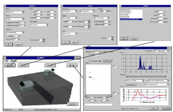
2. SUNDT
Figure 1 - The environment of the pre- and postprocessor SUNDT.
The computer program SUNDT has been developed to model some important situations in ultrasonic non-destructive testing of localised defects in an otherwise homogeneous and isotropic component. The PC based software is consisting of three major interactive parts: 1. The preprocessor where the simulation is specified.
2. The computational FORTRAN 77 kernel (UTDefect). 3. The postprocessor with the presentation of the result.
The UTDefect software [6][7] is a result of a research program at the Department of Mechanics, Chalmers University of Technology. The conversion from a scientific tool into a modern Windows-based simulation tool has been conducted by the SAQ Kontroll AB company. Both these projects have been financed by the Swedish Nuclear Power Inspectorate (SKI). The SUNDT program enables the commercial use (not only by a sparse number of specialists) of well documented solutions of some specific mathematical problems with an increasing number of validations and verifications. The UTDefect program has been compared to previous validations of existing simulation software [7] and also against experimental investigations [7][8][9][10]. The application is not restricted in any way to the Nuclear related industry but can be applied in other industrial societies using ultrasonic NDT.
3. THE KERNEL UTDefect
3.1 The Component
The simulated test piece is at the present state restricted to be of a homogeneous and isotropic material. All attenuation due to absorption (viscous effects) or grain boundary scattering is neglected. The component is (infinite plate with finite or infinite thickness) bounded by the scanning surface where one or two probes are scanning the object within a rectangular mesh. It is also possible to include a planar back surface, which for the strip-like crack may be tilted, but is otherwise assumed parallel to the scanning surface.
3.2 Available Defects
There are a number of defects of simple geometrical shape that can be chosen in UTDefect and most of them can also be located close to a planar back surface. Four volumetric defects are included: a spherical cavity, a spherical inclusion made of a isotropic material differing from the surrounding medium, a spheroidal cavity, and a cylindrical cavity. A circular
crack with the ability to specify the contact conditions across the crack surface is also
included. This enables a simulation of a situation where the crack is exposed to a background pressure and therefore being partly closed. The more commonly used models, open and fluid filled cracks, are also included as options. The circular crack can be arbitrarily placed and also rotated with two euler angles.
The above defects could be classified as models of manufacturing faults in the component where the circular crack could be the outcome of the rolling of a object containing a spherical inclusion. The main group of cracks appearing in connection with in-service NDT inspection, has the common characteristic of being initiated inside a pipe and propagating towards the scanning surface. If these cracks are longer than the ultrasonic beam width they could be approximated as a surface breaking strip-like crack assumed infinite in one direction parallel to the scanning surface, but perpendicular to the main scanning direction. The infinite strip-like
crack has been validated against defects fabricated by diffusion bonding methods [7][8][9]
while the surface breaking strip-like crack has been validated against manufactured fatigue cracks and EDM notches [7][8][9][10].
3.3 Calibration
In order to eliminate any differences due to the absolute amplitude level (corresponding to gain adjustment) it is appropriate, as in practical application of NDT, to use some kind of calibration procedure. The calibration in UTDefect is performed by a side-drilled hole (SDH) or a flat-bottomed hole (FBH). The calibration procedure with a SDH is treated exactly with the use of the cylindrical cavity while the FBH is approximated with an open circular crack. This approximation is expected to be valid close to specular reflection except at very low frequencies.
The calibration procedure consists of a line scan with the probe in pulse-echo situation nearby the point where one can expect maximum amplitude response, i.e. when beam axis hits the axis of the SDH or the centre of the FBH normally. The amplitude and the position of the peak response is noted and in addition the corresponding ”true” angle is calculated. The difference between the nominal (prescribed) angle and the generated ”true” probe angle is due to how the boundary conditions in the model has been deduced [6]. This effect is most significant for low frequencies and small effective areas (corresponding to small crystal sizes).
3.4 Probe Modelling
The probe is assumed to scan in a rectangular mesh over a flat surface of the component. The scanning can be performed by a single probe in a pulse-echo situation or a two probe arrangement either with fixed distance between transmitter and receiver or a positioned transmitter with the receiver scanning the prescribed measuring mesh.
The probe is modelled by an assumed effective area beneath the probe, used as boundary conditions in a half-space elastodynamic wave propagation problem. This enables an adaptation to a variety of realistic parameters related to the probe, e.g. wavetype, angle, crystal (i.e. size and shape) and contact conditions. In addition to the option of specifying the contact conditions it is also possible to suppress the ”wrong” wave type which enhance the possibility to make an interpretation of the received signal.
In order to reduce the computational effort, the integrals that appears in UTDefect are calculated approximately by the stationary phase approximation. This approximation is valid if the distance between the probe and the defect is many wavelengths and if the defect is outside the probe's near field domain. In order to reduce this limitation and to include the opportunity to model focused probes, the effective area modelling the probe is divided into a number (n) of rectangular probe elements (thus reducing the near-field length as 1/n2). In the present version of the software, line and point focus probes are available as options. The total signal response is than obtained by superposing contributions from all these minor elements which reduces the near field length but increases the computational time required. The modelling of probes both as transmitters and receivers is discussed in detail by Boström and Wirdelius [6]. The stationary phase approximation and its validity is also investigated.
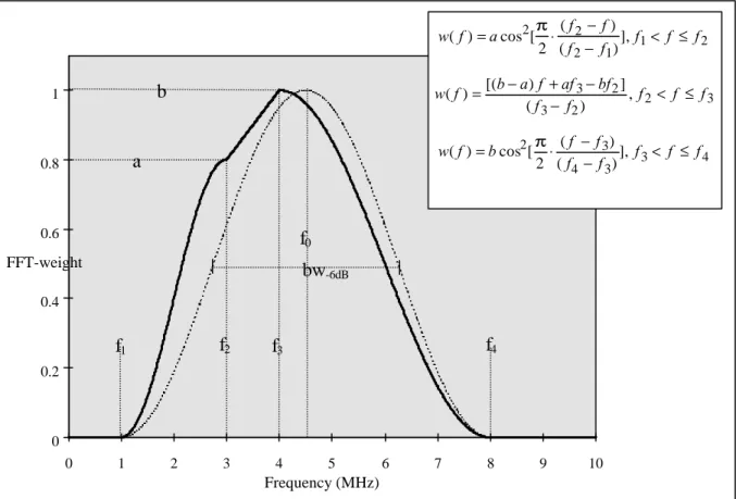
0 0.2 0.4 0.6 0.8 1 0 1 2 3 4 5 6 7 8 9 10
Figure 2 - Exampel of the frequency distribution function.
If time traces are required, the centre frequency and the 6 dB bandwidth are sufficient information and the program assumes a cosinesquare distribution (i.e. a = b = 1, the centre frequency f2 = f3 = (f4 + f1)/2 and the bandwidth (f4 - f1)/2 in figure 2) of the spectrum. If more detailed information about a specific probe's frequency spectrum is available, the program includes a more adaptable spectrum function. This function consists of two separate cosinesquare distribution functions (which may have different widths and heights) joined by a straight line (see figure 2).
3.5 Previous Validations
If mathematical modelling is to be used as an effective tool in any part of the qualification process the validation of the software has to be extensive and well documented. Every software that has been and will be developed inevitable include a range of validity which has to be investigated before it can be applied as a simulation of the reality.
Lakestani [3] reports on the comparison of three NDT simulation software with physical experiments on strip-like defects (fabricated by diffusion bonding), performed within the PISC III program. Two of the models used, are based on the geometrical theory of diffraction (GTD), i.e. the NDTAC and the Harwell TOFD software, and the third model is a boundary element method based model from the Kassel University. Results from the Lakestani report has been compared with UTDefect in Boström [7], Boström and Jansson [8] and Bövik and Boström [9]. In these reports the UTDefect also was compared with experimental results originated from set ups where surface breaking strip-like vertical cracks were situated in tilted back-sides. Both EDM notches with curved profiles [11] and full width notches [12] were used in the comparison.
w f a f f f f f f f w f b a f af bf f f f f f w f b f f f f f f f ( ) cos [ ( ) ( )], ( ) [( ) ] ( ) , ( ) cos [ ( ) ( )], = ⋅ − − < ≤ = − + − − < ≤ = ⋅ − − < ≤ 2 2 2 1 1 2 3 2 3 2 2 3 2 3 4 3 3 4 2 2 π π Frequency (MHz) FFT-weight f1 f2 f3 f4 a b f0 bw-6dB
Recently Eriksson et al [10] presented a validation of UTDefect using fabricated fatigue cracks (approximately shaped as parts of ellipses) in carbon steel plates. The corner echoes and the tip diffracted signals were included in the study and in general the simulations agree well with the experiments. Within this validation the limitation of the former probe model, regarding defects in the nearfield, was identified. A thorough investigation of the probe parameters and a comparison of the generated probe field with experimental data were also performed within the validation [10].
4. HOW TO RUN THE SUNDT PROGRAM
Before any execution can take place, please make sure that the system is compatible with your version of SUNDT (Windows NT 3.51). Please also make sure that the system, on the actual PC-station to be used, has the dot [.] as the decimal symbol (Control Panel/Regional Settings/Number). During the setup process the programs are to be placed within the same Folder beneath the the C:/-area. This includes the files SUNDT.exe and UTDef2.exe (kernel), the default pre-setting file indefa.txt and the list of available materials within the material.dat.
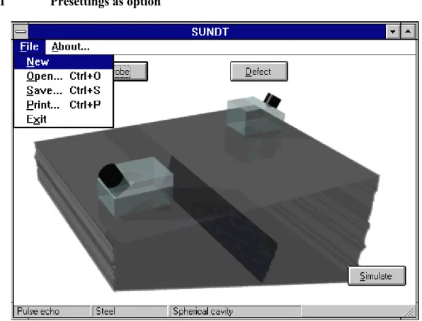
4.1 Presettings as option
Figure 3 - The Main-window in the preprocessor.
Previous executions could be used as a starting point for a new simulation. All information about a specific simulation are stored in the in”fileID”.txt file. The ”fileID” being a four letters, digits or a combination, is mutual for all in- and out- files. Together with the software, the package also include three in- files to be used as presettings. The in-files are being available (within SUNDT) using the Open option beneath File in the menu. Within the examples folder three possible presettings are available:
in0001.txt: Tandem configuration with two identical 58º longitudinal probes with centre frequency of 3MHz and 60% bandwidth. The defect is a 6mm surface breaking strip-like crack perpendicular to the backwall. The backwall is situated at a depth of 36 mm and is parallel to the scanning surface in this case.
in0002.txt: Same defect configuration as above but the probe is acting in a pulse echo situation.
in1001.txt: An unangled longitudinal probe acting in a pulse echo situation with centre frequency of 1MHz and 100% bandwidth. The defect is a spherical cavity (ø≈2mm) situated at a depth of 30mm without the influence of any
backwall.
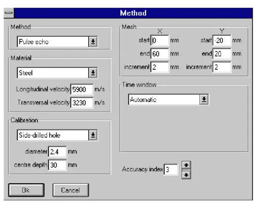
4.2 Available options within the Method-window
Figure 4 - The options available in the Method-window.
Method
There are three available combinations of probe configurations within the Method-window: • Pulse-echo with a single probe acting as both transmitter and receiver.
• Separate where the transmitter is placed at a defined coordinate while the receiver is prescribed to be positioned within the mesh (figure 5).
• Tandem configuration (used in TOFD applications) where the distance between transmitter and receiver is fixed while the movement of the couple (i.e. transmitter) is defined by the mesh option (figure 6).
Figure 5 - The definition of coordinates when Separate configuration is to be simulated.
Figure 6 - The definition of coordinates when Tandem configuration is to be simulated. (fixed)
Material
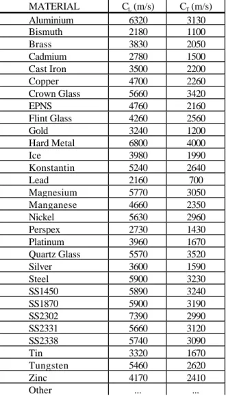
Together with the SUNDT program there is a enclosed file (material.dat) including a number of materials and their assumed wave speeds (table 1). These are available within the Method-window as a drag and drop option together with the possibilty of prescribing these material constants of the objekt that is to be simulated.
MATERIAL CL (m/s) CT (m/s) Aluminium 6320 3130 Bismuth 2180 1100 Brass 3830 2050 Cadmium 2780 1500 Cast Iron 3500 2200 Copper 4700 2260 Crown Glass 5660 3420 EPNS 4760 2160 Flint Glass 4260 2560 Gold 3240 1200 Hard Metal 6800 4000 Ice 3980 1990 Konstantin 5240 2640 Lead 2160 700 Magnesium 5770 3050 Manganese 4660 2350 Nickel 5630 2960 Perspex 2730 1430 Platinum 3960 1670 Quartz Glass 5570 3520 Silver 3600 1590 Steel 5900 3230 SS1450 5890 3240 SS1870 5900 3190 SS2302 7390 2990 SS2331 5660 3120 SS2338 5740 3090 Tin 3320 1670 Tungsten 5460 2620 Zinc 4170 2410 Other ... ...
Table 1 - List of available materials with defined wave speeds of longitudinal (CL) and shear waves (CT)
Calibration
In order to completely simulate the actual NDT situation, an option of calibration against a reference reflector, is included in the software. This also eliminates any hardware (i.e. ultrasonic equipment) related discrepancies between the model and the testing situation due to amplification. Possible reference reflectors are:
• Side-drilled hole • Flat-bottomed hole
Note though that the calibration is performed at the position with the peak response and the DAC method will be incorporated in a forthcoming version of SUNDT.
Mesh
The area (or line) on the object and the number of points that are to be scanned by the transmitter or receiver (due to chosen configuration) is specified within the Mesh frame.
Accuracy
In order to enable an optimisation of computational time without violating the accuracy of the simulation an option of altering an accuracy index is included. The value of this parameter can be placed between 1 and 5 with a default value of 3. If the parameter is increased this means extended computational time with a higher accuracy. The recommended procedure, if a large number of simulations is to be computed, is to increase the index number until enough accurate results are reached.
Time window
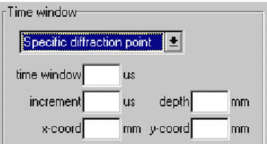
Figure 7 - The Time-window frame with an option of studying a specific diffraction point.
Based on information about the scanning mesh and the depth of the defect, the UTDefect sets the A-scan range in order to ensure a defect related signal being within the time window. If certain parts of the signal is to be gated out, the A-scan range can be specified within the Time-window frame. This will though be present for all the points within the scanning mesh. If the response from a specific point is of interest (e.g. tip diffraction) this can be filtered out by letting the program gating the Time-window into this point (figure 7).
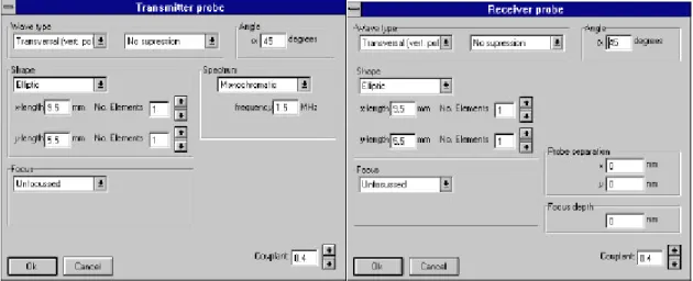
4.3 Specifying the parameters of the Probe(s)
If a pulse echo configuration has been selected in the Method-window all the probe related choices will be available beneath the probe option in the Main-window (figure 1).
Wave type and Angle
The nominal angle together with a prescription of generated wave type (longitudinal, transversal or horizontally polarised transversal) is to be specified in the Probe-window. This also include the possibility to suppress the nonspecified wave type, i.e. the transversal part when a longitudinal probe is to be modelled and vice versa.
Shape
The shape of the ”effective area” can be specified as elliptic or rectangular with an option of subdividing this area in order to reduce the nearfield length. If the Number of Elements are chosen to be in automatic mode this will make sure that the distance to any defect is larger than the distance of three nearfield lengths pointed out in previous validations [10] as a limitation of validity. The actual size of the ”effective area” as function of used crystal and prescribed angle has been studied by Eriksson et al [10]. It was found to be a reasonably good assumption to use the actual crystal size even when modelling angled probes.
Spectrum
The specification of the modelled frequency spectrum is performed within the Spectrum frame. The options are monochromatic (i.e. single frequency), cosine square distribution with a centre frequency and a prescribed bandwidth and a more adaptable spectrum function reach by the Input spectrum alternative. In the Input-spectrum window (figure 8) a number of discreate points are to be specified (more than 6) which by the Draw graph button generates the initial four frequencies (f1-f4) and two constants (a and b) which are the foundation for an approximative line adjustment:
w f a f f f f f f f a b a f f f f f f f b f f f f f f f ( ) cos [( ) ] [ , ] ( )( ) [ , ] cos [( ) ] [ , ] = − − ∈ + − − − ∈ − − ∈ 2 2 2 1 1 2 2 3 2 2 3 2 3 4 3 3 4 2 2 π π
The line adjustment together with the, by the user, provided discrete points (connected with lines) are visualised in a graph with the option of altering the frequencies and constants (see figure 2) in order to optimise the adjustment.
Couplant
In the Probe-window an option of changing the couplant constant (0≤ ≤δ 1, see [6]) is
available, enabling an influence of the distribution of generated wave types with the extreme cases of nonviscous fluid (δ=0) or glue (δ=1) as coupling medium. Within the previous reported experimental validation [10] this constant was found to best model normal conditions (i.e. water and waterbased gel) as it was put to 0.4 (default value).
Focus
The probe can also be provided with a line or a point focus function but with the consequence of an increasing number of subdividing elements.
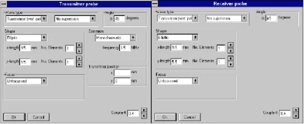
Figure 9 - The options in the Probe-windows as Separate configuration has been chosen.
Transmitter position
If the Separate probe arrangement (figure 5) has been chosen within the Method-window the single probe button in the Main-window is replaced by two separate buttons enabling different values of the parameters characterising the transmitter and receiver respectively (except for the frequency spectrum). The specification of the fixed coordinate of the transmitter for this configuration is to be prescribed within the Transmitter-window (figure 9).
Figure 10 - The options in the Probe-windows as Tandem configuration (TOFD) has been chosen.
Focus depth
If instead the Tandem configuration has been selected (figure 6) a focus depth can be specified (figure 10) which, based on the combination of probe angles, generates a specification of corresponding probe separation. Alternatively the probe separation can be specified and the corresponding focus depth is calculated.
4.4 Selection of Defect
There are a number of defects of simple geometrical shape that can be chosen in SUNDT (listed in table 2) and most of them can also be located close to a planar back surface.
Volumetric
Four volumetric defects are included: a spherical cavity, a spherical inclusion made of a isotropic material differing from the surrounding medium, a spheroidal cavity (figure 11), and a cylindrical cavity (same model is used when calibration is performed by a side drilled hole).
Figure 11 - Definition of the parameters that are to be specified for a spheroid.
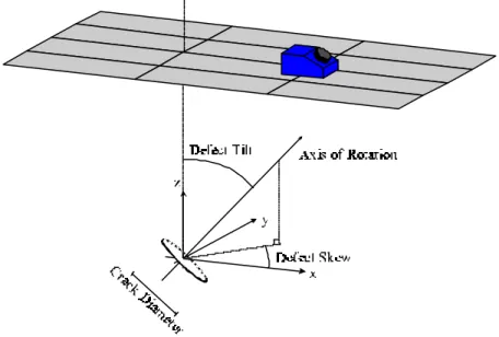
Circular crack
A circular crack (figure 12) with the ability to specify the contact conditions across the crack surface is included. This enables a simulation of a situation where the crack is exposed to a background pressure and therefore being partly closed. In order to model this situation the quotient between the background pressure,σ0, and the flow pressure, σf (which is about three times the yield stress), and the diameter of the contacts across the crack has to be specified (figure 14). For fatigue cracks typical values are thus 1-10% for stress quotient and 20 µm as the average contact diameter. The circular crack can instead of being partly closed, be prescribed as open (i.e. no presence of background pressure) or fluid filled. All these circular cracks can be arbitrarily placed with the ability of rotation with two euler angles (figure 12).
The above volumetric and circular defects could be classified as models of manufacturing faults in the component where the circular crack could be the outcome of the rolling of a object containing a spherical inclusion. The main group of cracks appearing in connection with in-service NDT inspection, has the common characteristic being initiated inside a pipe and propagating towards the scanning surface in a more or less specific direction. If these cracks are longer than the ultrasonic beam width they could be approximated as a surface breaking strip-like crack
Strip-like crack
The main group of cracks appearing in connection with in-service NDT inspection, has the common characteristic being initiated inside a pipe and propagating towards the scanning surface. If these cracks are longer than the ultrasonic beam width they could be approximated as a surface breaking strip-like crack assumed infinite in one direction parallel to the scanning surface, but perpendicular to the main scanning direction (figure 13). This strip-like crack can also be situated within the material, simulating lack of fusion.
Defect Specifications Limits* and Validations Comments Spherical cavity centre depth (mm)
diameter, d, (mm) d fc acc
s
<( ) [⋅ − ]
max
25 If back surface is present:
d c f acc s <( ) [⋅ − ] max 10 Corresponding window in figure 14
Spherical inclusion centre depth (mm) diameter, d, (mm) relative density (%) longitudinal velocity (m/s) transversal velocity (m/s) d c f s acc <( ) [⋅ − ] max 25 If back surface is present:
d c f acc s <( ) [⋅ − ] max 10 Corresponding window in figure 14
Spheroidal cavity centre depth (mm) diameter parallel, dpar, (mm)
diameter perpendicular, dper, (mm)
tilt (º ) skew (º ) 1 5< <5 d d par per max( , ) ( ) [ ] max d d c f acc par per < s ⋅ −9 Definitions of parameters found in figure 11 and
the window in figure 14
Circular crack centre depth(mm) diameter, d, (mm)
tilt (º ) skew (º ) open or fluid filled
d c f acc s <( ) [⋅ − ] max 10 [13] Definitions of parameters found in figure 12 and
the window in figure 14 Partly closed circular crack:
stress quotient(σ σ 0 f ) contact diameter d c f acc s <( ) [⋅ − ] max 10 [13]
Side drilled hole centre depth (mm)
diameter, d, (mm) d<(fcmaxs ) [⋅ −acc]
25
Strip-like crack centre depth (mm) width, w, (mm) tilt (º ) w c f s acc <( ) [⋅ − ] max 25 If back surface is present:
w c f acc s <( ) [⋅ − ] max 10 [7] [8] [9] Corresponding window in figure 14 Surface-breaking Strip-like crack centre depth (mm) width, w, (mm) defect tilt (º ) surface tilt (º ) w c f acc s <( ) [⋅ − ] max 25 [7] [8] [9] [10] Definitions of parameters found in figure 13 and
the window in figure 14
*All defects has to be at least two wavelengths (λ=c f ) or a probe (crystal) radius away from the probe(s). cs is the shear wavespeed, acc is the accuracy index in figure 4 and
fmax is the highest frequency in the spectrum (i.e. f4 or f0 + ∆f in figure 2).
4.5 Running the kernel
When all the settings are made the simulate button generates the necessary indata file for UTDefect and starts the computation (UTDef2.exe). Before the execution takes place it has to be provided with an identification (”fileID”) that has to be limited to four letters, digits or a combination, which then generates the file in”fileID”.txt. While the execution proceeds, a DOS-prompter is visible in the background (and corresponding DOS-window) which disappears as soon as the computation is done. The execution of UTDefect generates three files: ut”fileID”.txt, ut”fileID”.dat and ut”fileID”.dat.
The dat-files contains the results in binary format and are thus not available by any common text editor. The setting of parameters, specifying the simulation, are found in plain text within the ut”fileID”.txt file together with tabulated C-scan results (all A-scan information is excluded in order to limit the amount of information).
5 THE POSTPROCESSOR SUNDT
If the ut-files are pre-existing when an input file has been opened (see chapter 4.1) or an execution just has taken place, the option within the Main-window is extended with a result button (figure 15). This though implies that all the four files created by the program, with the same identity core (”fileID”), are placed within the same folder.
Figure 15 - The options in the Main-window when the result files are available.
The C-scans (figure 16) and distance-amplitude curves (figure 17) are all normalised and forced to be 0 dB at their maximum peak point. This point are in the upper left corner of the window specified to correspond either to a calibrated value or an absolute value. If calibration has been applied, the actual generated angle of the probe (”true angle”) is specified.
If a monochromatic simulation has been performed, a click by the pointer in the C-scan or the distance-amplitude curve makes it possible to identify the amplitude level for a single point. This point is visualised by a red circle in the C-scan (figure16) respectively by an arrow in the distance-amplitude curve (figure17) and the corresponding amplitude value is displayed in the window. Information of the settings, defining the actual simulation, is availble by the Info button (figure 17).
Figure 17 - The distance-amplitude curve as the result when a single line has been scanned monochromatically and the plain text information within the Info-window.
If instead time traces are of interest, at least the bandwidth has to be specified together with the centre frequency (see chapter 4.3). The computation of the time signal enables not only the A-scan information but also a visualisation of a B-scan. The time signal is reached in the same manner as the previous described identification of amplitude level for a single point. The scale of the A-scan graph can be altered between automatic amplitude scaling (individually maximized) or the absolute value of the amplitude being between 0 and 1. The default time signal (δ ) is unrectified but it is possible to use a number of filtering functions: Full-wave rectified (δ ), positive Half-wave rectified ((δ δ+ ) /2 ), negative Half-wave rectified ( (δ δ− ) /2 ) and the posibility to reduce all signals below a specified level in a Full-wave rectified time signal. It is also possible to change the time unit from microseconds into sound path length in mm (based on CL or CT specified in the Method-window).
Figure 18 - The A- and C-scan information within the Result-window when an area has been scanned with a pulse (a time window).
In order to generate a B-scan, the ”Line marker visible” option-box above the graph has to be marked. The B-scan is then defined by a line in the C-scan which is generated by the left mouse button indicating its start and correspondingly the right mouse button defining its end (figure 19). The time window presented in the A- and B-scans can be altered by using the mouse buttons, in the same manner as above, applied on the ”Time Gate” line.
The ”Create B-scan” button then visualise the B-scan with the time axis beginning at the top of the B-scan and ending at the bottom with the range displayed at its right side. Corresponding geometrical axis is defined at the bottom of the B-scan and includes a scroll possibility which alters the displayed A-scan information. This point is indicated in the C-scan as a blue circle (figure 19) or an arrow in the case of a distance-amplitude curve (figure 20).
Figure 19 - The information represented by the B-scan is defined by a line in the C-scan and a specification of the time window (Time Gate).
Figure 20 - The information represented by the B-scan is defined by a line in the C-scan and a specification of the time window (Time Gate).
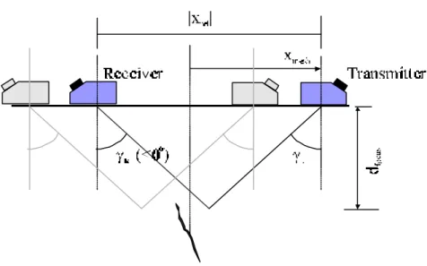
Figure 21 - Definition of the distances S1-S6 and the angles γ1-γ3 used in the calculation of possible axial ray paths when the surface breaking crack is used as defect in the simulation.
Due to the complexity and the variety of multiple reflection possibilities that are present when the defect consists of a surface breaking crack, an option that enables an identification of possible axial ray paths in a corresponding A-scan has been included. The definitions of the distances S1-S6 and angles γ1-γ3 are found in figure 21 and corresponding specification of the calculated wave paths, that are found within in the Sound paths-window, are tabulated in table 3. The calculation (figure 22) just stipulate the expected travel time and doesn’t quantify any amplitude from the various contributions to the signal.
The contribution that is based on a transversal wave hitting the backsurface, converted and thereafter reflected by the crack-surface as a longitudinal wave (T3→L4→L1, i.e. TLL), or vice verse, is in the program restricted to be deduced by the probe within its ”effective area” (see chapter 4.3). One of the contributions is based on an assumption of a transversal wave hitting the surface at the critical angle, generating a creeping wave which then is reflected by the corner as a longitudinal (T3→L6→L2) and a transversal wave contribution (T3→L6→T2). Numerical experience has revealed that significant components of the signal response, are parts that has been converted into a Rayleigh wave at the corner, travelled along the crack surface as a Rayleigh wave and thereafter been reflected at the corner back to the probe (L2 -R5-R5-L2 and T2-R5-R5-T2). These parts are (by the model) quantitatively comparable with the tip diffracted wave contributions.
Designation History
L1-L1 tip diffracted longitudinal wave
L2-L2 corner echo (longitudinal)
L2-R5-L1 longitudinal wave hitting the corner, yielding a Rayleigh wave which diffracts from the tip as a longitudinal wave
L1-R5-R5-L1 a longitudinal wave, converted into a Rayleigh wave at the tip, travelled along the crack surface as a Rayleigh wave and thereafter been diffracted as
a longitudinal wave at the tip back to the probe
L2-R5-R5-L2 a longitudinal wave, converted into a Rayleigh wave at the corner, travelled along the crack surface as a Rayleigh wave and thereafter been reflected as
a longitudinal wave at the corner back to the probe T3-L4-L1 transversal wave hitting the backsurface, converted and thereafter
reflected by the crack as a longitudinal wave
T3-L6-L2 transversal wave hits the backsurface at critical angle generating a creeping wave which is reflected by the corner as a longitudinal wave L1-T1 tip diffracted converted wave
L2-T2 corner echo (converted)
L2-R5-T1 longitudinal wave hitting the corner, yielding a Rayleigh wave which diffracts from the tip as a transversal wave
L1-R5-T2 transversal wave hitting the corner, yielding a Rayleigh wave which diffracts from the tip as a longitudinal wave
L1-R5-R5-T1 a longitudinal wave, converted into a Rayleigh wave at the tip, travelled along the crack surface as a Rayleigh wave and thereafter been diffracted as
a transversal wave at the tip back to the probe
L2-R5-R5-T2 a longitudinal wave, converted into a Rayleigh wave at the corner, travelled along the crack surface as a Rayleigh wave and thereafter been reflected as
a transversal wave at the corner back to the probe T1-T1 tip diffracted transversal wave
T3-L6-T2 transversal wave hits the backsurface at critical angle generating a creeping wave which is reflected by the corner as a transversal wave
T2- T2 corner echo (transversal)
Figure 22 - Calculation of possible sound paths as function of: probe position x (A-scan point), thickness of scanned object D, tilt of surface β, width of crack S5 and tilt of crack α.
6 AN EXAMPLE
The simulation described in this chapter is used as a demonstration of how the handling of the SUNDT software is conducted. In the Method-window (figure 23) the actual scanning is specified. This also include definitions of the wave speeds in the object and what kind of calibration that should be applied. Since the tandem configuration has been chosen as the measurement system, both transmitter and receiver parameters has to be specified which also includes the distance between the probes (figure 6). Since the tandem configuration has been selected a focus depth can be specified (figure 10) which, based on the combination of probe angles, generates a specification of corresponding probe separation.
Figure 23 - The settings in the (in this case) four different windows.
The surface breaking crack is selected as defect and in the Defect-window it is specified to be of 6mm width and placed perpendicular to the, at 36mm depth placed, backsurface (this being parallel to the scanning surface). The often small discrepancy between specified nominal angle and the actual generated angle is though in this situation of vital importance. In this example a couple of 55º probes are requested to have a focus depth of 30mm in order to optimise the signal due to tip diffraction. In order to achieve this, the probes has to be applied with 58º angles and separated 86mm (nominal focus depth of 27mm).
Figure 24 - The presentation of the result as A-, B- and C-scan from the simulated example.
After the calculation, based on the settings previous described (figure 23), the result is visualised as A-, B- and C-scans. The C-scan (in this case a distance-amplitude curve) is automatically drawn when the Result-window is activated. The axes in the C-scan are predefined by the mesh in the preprocessor and an amplitude range from 0dB down to -40dB. The B-scan is defined by indicating a line in the C-scan and setting the time window with the time gate option (see chapter 5). The arrows below the B-scan makes it possible to step to the closest A-scan and the scroll function enables the possibility to pick up any individual A-scan from within the B-scan. The current position for the presented A-scan is indicated in the C-scan by (in this case) an arrow along the B-scan line and in the B-scan by the scroll bar.
The A-scan position studied in figure 24 is the point where one would expect maximum tip diffracted signal. This contribution is identified (17.5µs) and its amplitude is about 10% of the maximum value in the C-scan (0.2dB more than SDH) which than corresponds to 19.8dB below reference level (i.e. δ δ= cal+δgraph =0 2. + −( 20)). The model of the surface breaking crack is mathematically a crack with an infinitesmal distance to the surface which permits waves to travel over the crack opening. This false ”corner echo” is found in figure 24 at 19µs and has the amplitude of about 80% of the maximum value in the C-scan which than corresponds to 1.7dB below reference level (i.e. 0.2-1.9dB).
For every calculation there is also a file generated in plain text format, which include the choices of parameters defining the simulation and the corresponding C-scan results. This text information is reached within the Result-window by the Info button and the file can also be read by any simple text-editor.
REFERENCES
[ 1 ] Chapman, R.K., ”A system model for the ultrasonic inspection of smooth planar cracks”, J. Nondestr. Eval. 9, 127-211 (1990).
[ 2 ] Fellinger, F., Marklein, R., Langenberg, K.J. and Klaholz, S., "Numerical modeling of elastic wave propagation and scattering with
EFIT-elastodynamic finite integration technique", Wave Motion 21, 47-66 (1995).
[ 3 ] Lakestani, F., ”Validation of mathematical models of the ultrasonic inspection of steel components”, PISC III report No 16, Joint Research Centre, Institue of Advanced Materials, Petten, The Netherlands (1992).
[ 4 ] Gray, J.N., Gray, T.A., Nakagawa, N. and Thompson, R.B.,
”Nondestructive evaluation and quality control”, Metals Handbook 17, ASM International, Ohio (1989).
[ 5 ] Achenbach, J.D., ”Measurement models for quantitative ultrasonics”,
J. Sound Vibr. 159, 385-401 (1992).
[ 6 ] Boström, A. and Wirdelius, H., ”Ultrasonic probe modeling and
nondestructive crack detection”, J. Acoust. Soc. Am. 97, 2836-2848 (1995).
[ 7 ] Boström, A., ”UTDefect - A computer program modelling ultrasonic NDT of cracks and other defects”, SKI Report 95:53, Stockholm (1995).
[ 8 ] Boström, A. and Jansson, P-Å., ”Developments of UTDefect: rough cracks and probe arrays”, SKI Report 97:28, Stockholm (1997).
[ 9 ] Bövik, P. and Boström, A., ”A model of ultrasonic nondestructive testing for internal and subsurface cracks”, J. Acoust. Soc. Am. 102, 2723-2733 (1997).
[ 10 ] Eriksson, A.S., Boström, A. and Wirdelius, H., ”Experimental validation of UTDefect”, SKI Report 97:1, Stockholm (1997).
[ 11 ] Becker, F.L., Doctor, S.R., Heasler, P.G., Morris, C.J., Pitman, S.G., Selby, G.P. and Simonen, F.A., ”Integration of NDE reliability and fracture
mechanics”, NURE/CR 1696, PNL-3469, U.S. Nuclear Regulatory Commission (1981).
[ 12 ] Chapman, R.K., private communication (1994).