Numerical analysis and model updating of a steel-concrete composite bridge: Parametric study & Statistical evaluation

(1)

Numerical analysis and model updating of a

steel-concrete composite bridge

Parametric Study & Statistical evaluation

ABDULRAHMAN KEIWAN POTRUS FADI

Master’s Thesis at the Division of Structural Engineering and Bridges

June 2015

TRITA-BKN. Master Thesis 462, 2015 ISRN KTH/BKN/B-462-SE

(2)

©Keiwan Abdulrahman & Fadi Potrus 2015 Royal Institute of Technology, KTH

Department of Civil and Architectural Engineering Division of Structural Engineering and Bridges Stockholm, Sweden, 2015.

(3)

Acknowledgements

First and foremost, we would like to express our sincere gratitude to our supervisor, John Leander, researcher at the division of Structural Engineering and Bridges at KTH, for his support and assistance throughout our studies. His guidance and advice have been a great asset in our progress of writing this thesis. A big thank you to our examiner, Professor Raid Karoumi, head of the division of Structural Engineering and Bridges at KTH.

We would also wish to thank our families, for their support, their advice and their patience throughout our years as students at KTH. A big thank you to our fellow students, friends and teachers who made these years at KTH unforgettable.

Stockholm, June 2015 Keiwan Abdulrahman Fadi Potrus

(4)

(5)

Abstract

In the year 2006, only 10 years after the steel- concrete composite bridge, Vårby bridge was built, fatigue cracks were found during an inspection. To further inves-tigate the reasons and the potential danger of the cracks, an investigation under the commission of the Swedish Transport Administration was issued in 2009. Af-ter the detection of fatigue cracks, several measurements were carried out in order to monitor the statical behaviour by the use of strain gauges at selected positions along the bridge. The measurements from the strain gauges monitoring the global behaviour were then used to calibrate an finite element model.

The present report is part of the research of understanding the behaviour of steel-concrete composite bridges. Numerical analysis and model updating have been used in order to understand and determine how different parameters affects the strain range and the global behaviour. The numerical analysis and parameter study were performed in the Finite Element software Abaqus and programming language Python. The outcome of the parameter study was then used to perform the model updating by the method of falsification in MATLAB.

The results from the parameter study and the model updating showed that the measured strains could be reached with a wide range of parameter combinations. Even with unreasonable parameter values, the measured strains were obtained. To investigate the reason for this, a multiple linear regression analysis was performed which showed that the strain range is strongly correlated to the Young’s modulus of steel and concrete and also to the connector elasticity, which resembles the studs in the real bridge.

Two different finite element models, with two completely different input parameter values, obtain the same strain range for the global behaviour. It is therefore not certain to assume that a model is accurate and valid based on the fact that the predicted strain range from the finite element model is close to the measured strain range since the global behaviour of a steel- concrete composite bridge can be mod-elled by many different sets of parameters.

Author keywords: Model updating; Finite element method; Parameter study;

Abaqus; Falsification; Fatigue; Composite bridges; Monitoring; Measurements; Strain range; Global behaviour

(6)

(7)

Sammanfattning

År 2006, endast 10 år efter att samverkansbron i stål och betong, Vårbybron, färdigställts, fann man utmattningssprickor under en inspektion. För att ytterligare utreda orsakerna bakom sprickorna inleddes en utredning ledd av Trafikverket år 2009. Efter upptäckten av utmattningssprickor placerades flertalet töjningsmätare ut på bron. De uppmätta globala töjningarna användes sedan för att kalibrera en finita elementmodell.

Den här rapporten är en del av forskningen i att förstå det globala beteendet för en samverkansbro i stål och betong. Numerisk analys och modeluppdatering har använts för att förstå och fastställa hur olika parametrar påverkar det globala be-teendet. Den numeriska analysen och parameterstudien har utförsts i finita ele-mentprogrammet Abaqus och programmeringsspråket Python. Utdata från param-eterstudien användes sedan för att utföra en modelluppdatering genom metoden falsifiering som utfördes i MATLAB.

Resultaten från parameterstudien och modeluppdateringen visade att dem upp-mätta töjningarna kunde nås för ett stort antal parameterkombinationer. Även för orimliga parametervärden kunde dem uppmätta töjnignarna nås i modellen. För att vidare studera detta gjordes en regressionsanalys som visade att töjningsvidden och parametrarna är starkt korrelerade och att töjningsvidden är linjärt beroende av parametrarna.

Två olika finita elementmodeller, med två helt olika val av parametrar ger samma utslag på töjningsvidden för det globala beteendet. Det är därför inte säkert att anta att en modell är giltig baserat på att modellen kan uppnå de uppmätta töjn-ingsvidderna, eftersom det globala beteendet för en samverkansbro i stål och betong kan modelleras med flera olika parameterkombinationer.

Nyckelord: Modeluppdatering; Finita element metoder; Parameterstudie; Abaqus;

Falsifiering; Utmattning; Samverkansbroar i stål och betong; Fältmätningar; Töjn-ingsvidd; Globalt beteende

(8)

(9)

Introduction

1.1 Background

The Vårby Bridge, built in 1996, is located south of Stockholm and serves as a highway bridge on the E4. The bridge has been under attention since the detection of fatigue cracks during an inspection in 2006 [1]. To identify the reasons and the potential danger of the cracks, an investigation under the commission of the Swedish Transport Administration was issued in 2009 [2]. Several other investigations of the bridge have been carried out since then in order to determine the reason/reasons for the developed cracks and to prevent these from propagating further [3].

Ongoing research is carried out regarding Model updating in the field of dynamic analysis were measurements are used in order to reach concordance with Finite El-ement models.

This master thesis is part of the research of understanding the behaviour of steel-concrete composite bridges using numerical analysis, measurements and model up-dating in order to determine the important parameters affecting the global be-haviour.

The outcome of this thesis will give a deeper understanding on how the strain range varies in such a bridge by varying different parameters. Fatigue cracks are largely dependent on the stress range, the maximum and the minimum stress in a load cycle. Thus the important parts of the global behaviour of the bridge, to study with varying parameters, are the lowest and highest stresses. This will give a better understanding of how the stress range in a steel-concrete composite bridge changes by varying the parameters. The strain range is related to the stress range through the Young’s modulus of the material when studying uniaxial normal stresses and since the Young’s modulus of the materials are varied in the parameter study, it is more correct to study the strain range instead of the stress range.

(12)

2 CHAPTER 1. INTRODUCTION

1.2 Approach

This thesis has been subdivided into four chapters. The first chapter contains a brief introduction of this thesis, the aim and scope, and finally a review of previous works regarding the Vårby bridge.

The second chapter deals with the method used for this thesis. To investigate and be able to run the parameter study which will consist of a large amount of simulations, a fast model is of vital importance. A Finite Element model is created using the finite element software Abaqus. When the model is fast and accurate enough compared with measurements, a Python script is created to run the parameter study. The script in Python is modified and compiled in such a way that it runs the solver in Abaqus and writes the result from all the simulations to a text file. A MATLAB script is then created to retrieve the desired results. The results are then interpreted and a statistical evaluation is carried out by the method of falsification. Since the model must be created in such a way that the parameters can easily be modified, simulations of small scale models in the pre-modeling phase are necessary. The general steps of this master thesis can be illustrated in figure 1.1. This is of course a general illustration of the process in this thesis and more of a guideline than a rule.

Figure 1.1: A general illustration of the approach in this thesis.

1.3 Aim

The aim of this study is to carry out a statistical evaluation of the different pa-rameters in a composite steel-concrete bridge in order to understand how much of an impact each parameter has on the strain range. This is performed using nu-merical analysis in the Finite Element software Abaqus. An finite element model is created in such a way that it is possible to modify the code of the model using programming software MATLAB and Python in order to make it more efficient to run several simulations of the model with different values of each parameter. After the statistical evaluation, using the method of falsification, it is possible to deter-mine which parameter/parameters that is of importance for such a bridge. Some

(13)

1.4. SCOPE 3

examples of the evaluated parameters are the Young’s modulus of the materials of the bridge and the different characteristics of the bridge.

1.4 Scope

The scope of this thesis are defined by the following bullets:

• The bridge is modelled in the Finite element software Abaqus were different structural element types are modeled in order to decrease the computation time. The section of the bridge analyzed is in the second to last span where strain gauges have been placed. The measurements used are from strain gauge 8 according to Figure 3.4a. The quantities used from the measurements are strains of the main girders in the bottom flange.

• The passing vehicle, used for the measurements, is a lorry of known weight according to figure 4.13 in section 4.3.

Several limitation is carried out throughout the report for different reasons, some of them are:

• Beam elements used for the part of the bridge with less influence, section 4.2 • Shell elements for the part of the bridge with greater influence, section 4.2 • No plastic analysis

• No dynamic analysis

(14)

(15)

Chapter 2

Model updating

Model updating in the field of finite element modeling is the process of ensuring that the finite element analysis results in a model that better reflect measured data than the initial model. Essentially, finite element model (FEM) updating is a technique of estimating parameters [4]. It is based on updating parameters which are uncertain to get reasonable agreement between the experimental measured model and the finite element model. The updated model can then be used for further analysis, computation and even damage detection [5]. The approach is frequently used in the field of mechanical engineering, aerospace engineering, et. al, and focusing mainly on the application of the dynamical parameters such as the mode shapes and the frequency response functions in the finite element model updating process [6]. Static parameters are however more amenable to the modeling of complex structures, hence static properties of structures are also widely studied such as displacements and strains.

Essentially the model updating procedure can be described in three steps [7]. • Selection of ’responses’ as reference data, normally the measured data, such

as strains, frequencies and mode shapes.

• Selection of parameters to update, to which changes the selected responses should be sufficiently sensitive and uncertain.

• Model tuning which is the iterative process of modifying the selected param-eters based on the selected reference data.

2.1 Quasi-static Generalized Influence Line

Jingbo Liaoa, Guangwu Tanga, et, al. [6], made a study to further develop an approach on finite element model updating based on the quasi-static generalized influence line (QSGL).

The damages were simulated on three beams of different geometrical groove accord-ing to figure 2.1, to illustrate the induced local changes of the bendaccord-ing stiffness EI

(16)

6 CHAPTER 2. MODEL UPDATING

at the zone of the damage. The Young’s modulus for the beams were 2.76x103MPa. The perfect model, without damage, model A, was then compared to the others. The beams were subjected to a concentrated force to produce the deflection influence line of the mid-span M. The obtained displacement of the damaged and undamaged beam is shown in figure 2.2. In both damage models, the minimal deflection values derives from that of a perfect undamaged model. This is because of the decrease in rigidity of the damaged models, which in turn gives good agreement with the an-alytical results. For a 2-D beam element, different geometrical rectangular groove results in a decrease in the moment of inertia, hence the grooves were modeled with a equivalent bending rigidity. The equivalent bending stiffness was normalized by the initial bending stiffness and was chosen as the updating parameter.

Figure 2.1: The perfect model A, the damaged model B and the damaged model C, units in mm [6].

Eq. 2.1 shows the updating function used in the report by Jingbo, Guangwu, et. al.

(17)

2.1. QUASI-STATIC GENERALIZED INFLUENCE LINE 7

Figure 2.2: Deflection of the mid-span point M for the experimental model A, B and C [6].

Figure 2.3: Comparison of the initial, updated and measured influence lines for model B and model C [6]. Fz(x) = N X k=1 M X i=1 (Zci− ηZT i)2 ZT i (2.1) Where, N is the total number of influence line test points, M is the total number of load steps, ZT i and Zciis the measured and calculated influence line, γi is a weight

(18)

8 CHAPTER 2. MODEL UPDATING

Table 2.1: Measured and updated bending stiffness of the damaged model B and C [6]. EI in N m2 _{and Error in %.}

Damaged zone Measured value EI Updating value EI Error

Left side of model B 23.66 23.40 -1.10

Right side of model B 23.66 23.53 -0.56

Left side of model C 23.66 23.21 -1.94

Right side of model C 28.72 26.68 -0.17

The initial and updated values are presented in figure 2.3 and table 2.1. The results demonstrated by Jingbo, Guangwu, et. al, shows that the updated finite element model, with the updating function used, fits very well to the experimental model and hence can be used in practical engineering fields, especially for bridges.

2.2 Implementation of model updating

There are a number of techniques of significance to consider in order to implement a successful model updating method [7].

• It is important to understand that the finite element model for model updating differs from a conventional finite element model such that it is important to model the structure with as much detail as possible to represent the geometric and structural form for the location that is of significance for the intended parameters to be updated.

• The selected parameters should be sensitive to the selected response and must be uncertain properties. Sensitivity analysis combined with sound engineering is a good way to determine the sensitive parameters.

• Limited manual updating based on trial and error is necessary in order to obtain suitable initial values of selected parameters as a starting point for model tuning.

(19)

Chapter 3

The Vårby Bridge

The bridge is a highway bridge spanning the northern part of Fittja Bay with a length of roughly 255 meters. Designed between 1994 and 1996 by Rundquist Ar-chitects the bridge consists of two parallel bridges having three lanes and a shoulder on each bridge were the northern bridge is the one studied in this thesis. The to-tal width of the northern bridge is 15 meters with a vertical clearance of 6 meters for boats and the like. The bridge is a steel-concrete composite bridge supported by seven supports carrying the longitudinal beams which in turn are carrying the concrete deck having approximately 50.000 vehicle passing it every day. A photo of the bridge is presented in figure 3.3. The composite action is carried out by studs welded to the flanges of the longitudinal beams connecting the concrete deck to the girder. Figure 3.1 and 3.2 shows the elevation and the cross section of the bridge.

Figure 3.1: Elevation of the bridge.

(20)

10 CHAPTER 3. THE VÅRBY BRIDGE

Figure 3.2: Cross section of the bridge.

(21)

3.1. MEASUREMENTS 11

3.1 Measurements

After the detection of fatigue cracks, measurements have been carried out in order to monitor the static behaviour in the web stiffeners [3]. Strain gauges have been placed at selected positions and then used as calibration of a finite element model. Two types of measurements have been carried out, one with a lorry of known weight passing the bridge at different positions and the second is long-term measurements over several days caused by random traffic [3]. The measurements used in this re-port is of the first type in order to calibrate the finite element model.

To investigate the global behaviour, the strains of the bottom flange of the longitu-dinal beams were monitored, strain gauge 4- and 8, according to figure 3.4a. The measurements used in this report is the gauge monitoring the strains located at the bottom flange of the longitudinal beam following grid D, gauge 8. The location of the gauges at the main girder relative to the total bridge is in the second last span, between span 5 and 6 as can be seen in figure 3.4b.

The short term measurements for a vehicle of known parameters such as weight, speed and position were carried out in June 2009. As the traffic was intense and the bridge couldn’t be closed, the measurements were performed during night time [2]. The vehicle used in the measurements can be seen in figure 4.13.

3.2 Previous works

Several studies and investigations has been carried out regarding the Vårby bridge over the years. They have however almost exclusively been handling the issue of fatigue. No investigation regarding the parameters affecting the global behaviour of the bridge has been made in the past.

Three reports have been studied in more detail for this thesis;

The first one is from Projekt Engagemang in Stockholm [3] and concerns the surements carried out on the bridge. The report, giving the results from the mea-surements is then used to calibrate a finite element model created and analysed by Luleå University of Technology [8].

The third report is a FE-analysis of the Vårby bridge, investigating the fatigue cracks on the bridge, done by Chalmers University of Technology [9]. The report states that a load positioned over a longitudinal beam results in high compressive stresses, which combined with residual stresses from the welding on the web stiff-eners results in a load cycle that could be the reason for the cracks. However the authors also states that the interaction between the concrete deck and the steel girder was not modeled correct in Abaqus in order to retrieve good and accurate results.

(22)

12 CHAPTER 3. THE VÅRBY BRIDGE

(a) The location of the strain gauges on the main girders, [3].

(b) The location of the strain gauges between span 5 and 6.

(23)

Chapter 4

Finite element model

4.1 Abaqus

Abaqus is a powerful engineering software using the Finite Element Method to solve problems ranging from smaller linear simulations to complex and challenging non-linear simulations. It is used for modeling all kinds of materials from metals, rubbers and polymers to reinforced concrete, composites and geotechnical materials. It is a general-purpose software and can not only solve stress/displacement problems but other areas such as heat transfers, acoustics and fluid dynamics.

The software consists of two types, Abaqus/Standard and Abaqus/Explicit where the first one, which is used in this report is used for solving linear and nonlinear static/dynamic problems and the latter using explicit dynamic finite element for-mulation and is used for modeling transient dynamic events such as impacts and blast problems.

The software can be run from the CAE (Complete Abaqus Environment) which is an interactive graphical environment that allows models to be created and edited in a user friendly manner.

Another way to run Abaqus is to create the model trough the input file and send it directly to the solver without having to use the CAE [13].

Implicit/Explicit

In general, a linear static problem, which is the case of this thesis, is preferably solved by using the implicit method. However, for problems that can be solved using both methods, it is important to understand the different characteristics of the implicit and explicit procedure in order to be able to determine which method that is appropriate for the given problem. The main difference between the two is that the implicit method is a stiffness-based solution technique that is unconditionally stable while the explicit method uses a conditionally stable explicit integration technique. If the problem have difficulties converging because of various contact or material complexities which will result in a large number of iterations, Abaqus/Explicit might

(24)

14 CHAPTER 4. FINITE ELEMENT MODEL

be a choice to consider since such problems requires a large set of linear equations to be solved in Abaqus/Standard. This is not the case for analyzing the global behaviour of the Vårby bridge, and therefore using Abaqus/Standard is the natural choice for this thesis [13].

From Input to Output

As mentioned earlier, the input file contains a complete description of the model in the form of lines of code. This is the communication between the solver in Abaqus and the pre-processor CAE.

The input file is build up of two sections, the first is data defining the structure being analyzed, and the second section contains information about history data, defining what happens to the model, for example the load for which the response of the structure is required. Having the model in the form of code in an input file allows the user to modify the model trough a text file. This is one of reasons why the authors of this report are using Abaqus. To do a parameter study in a complex finite element model by manipulating the input file is vital. By using scripting, in programming languages such as MATLAB and Python, it is possible to do iterative steps and run large amount of simulations very effectively.

More about the parameter study, the MATLAB and Python scripting are presented in their respective sections later in this report.

4.2 Use of elements

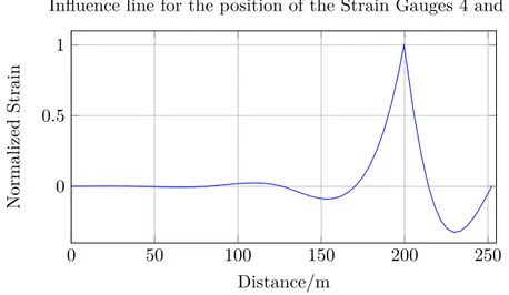
As previously stated in section 1.3, the parameter study is one of the final steps in this thesis. In order to have a fast and effective model, the choice of elements is important. Depending on the type of element, the total simulation time can change significantly. Different elements have different number of nodes and degrees of freedom, and thereby more or less equations to solve. It is important to model the bridge in such a way that elements with less nodes and degrees of freedom is used at the locations where there are no or less influence for the strains at the point of interest. This can be illustrated by a simple influence line at the point of the location of the strain gauges 4 and 8, see figure 4.1.

Figure 4.1 shows the influence line for the bridge assuming a constant stiffness over the spans. The spans of greater influence for the point of interest is the span where the gauge is located and the spans to the left- and right of it. It is therefore suitable to use beam elements for the spans where there are no or less influence and shell elements for the span/spans with greater influence. The difference between the two elements is described in detail in the next section.

(25)

4.2. USE OF ELEMENTS 15 0 50 100 150 200 250 0 0.5 1 Distance/m Normalized Strain

Influence line for the position of the Strain Gauges 4 and 8

Figure 4.1: A simple influence line showing the strain at the position of the strain gauges.

Beam elements

Beam elements are preferably used for the spans with less influence on the result to minimize computational time and are used for the main-girders for all spans along the bridge except for the span where the strain gauges are located, i.e. span 5-6 where shell elements are used instead for the main girder. Beam elements are also used for the crossbeams in all spans.

Beam elements are defined by a line, or a wire, as it is called in Abaqus, with a node in each end. In a 3D beam, each node has 6 degrees of freedom, see figure 4.3. A 2D beam will in comparison to the 3D beam, only have translations and rotations along the x and y axis while the 3D beam will also include the z axis. Since the entire element is defined by a line, increasing the mesh will only increase nodes and hence more degrees of freedom along the line [12].

Depending on whether the section integration is performed before or during the analysis, different material definitions are required in Abaqus. In a linear-elastic problem, the deformations are assumed to be small and the material properties is therefore assumed to stay the same during the entire analysis. Thus the integra-tion is performed before the analysis compared to a non-linear analysis with large deformations not having a linear material behaviour, where the integration is an iterative process during the analysis.

In an integration performed before the analysis the cross sectional geometry and the material properties of the beam is assigned to the element, such as the Young’s modulus E and Poisson’s ratio υ. The input parameters used in the finite element model is described in detail in section 5

(26)

the web along the bridge, see figure 4.2. This is modeled by defining different cross sections between every crossbeam having a constant height calculated as an average height of the longitudinal beam between two crossbeams. The flange thickness of the longitudinal beams also varies along the bridge and are modeled with a constant thickness between every crossbeam. The thickness of the flanges changes at joints and an interpolated value is used in the model for those parts. The modelled girder and the specific cross sectional values is presented in table 4.2. Figure 4.5 shows the main girder together with the crossbeams in the finite element model.

Figure 4.2: Tapered main girder.

Figure 4.3: A 3D Beam element with 6 degrees of freedom, u, v and w being translations and θx, θy, θz rotations around their respective axis [12].

Main girder modeled with beam elements

For the main girder modelled with beam elements, a total of 28 different types of I-beams are modelled with cross sectional values presented in table 4.1 with notations according to figure 4.4.As stated previously, all span except the span between supports 5 and 6 are modeled with beam elements.

(27)

4.2. USE OF ELEMENTS 17

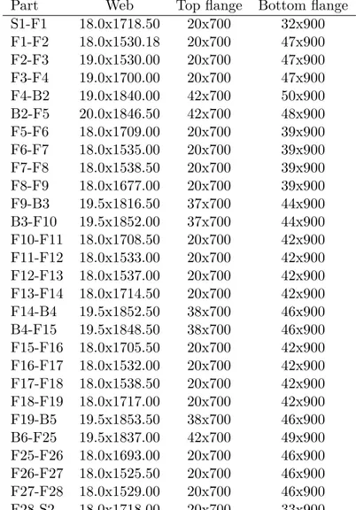
Table 4.1: The cross sections of the longitudinal beams along the bridge. All values are given in mm.

Part Web Top flange Bottom flange

S1-F1 18.0x1718.50 20x700 32x900 F1-F2 18.0x1530.18 20x700 47x900 F2-F3 19.0x1530.00 20x700 47x900 F3-F4 19.0x1700.00 20x700 47x900 F4-B2 19.0x1840.00 42x700 50x900 B2-F5 20.0x1846.50 42x700 48x900 F5-F6 18.0x1709.00 20x700 39x900 F6-F7 18.0x1535.00 20x700 39x900 F7-F8 18.0x1538.50 20x700 39x900 F8-F9 18.0x1677.00 20x700 39x900 F9-B3 19.5x1816.50 37x700 44x900 B3-F10 19.5x1852.00 37x700 44x900 F10-F11 18.0x1708.50 20x700 42x900 F11-F12 18.0x1533.00 20x700 42x900 F12-F13 18.0x1537.00 20x700 42x900 F13-F14 18.0x1714.50 20x700 42x900 F14-B4 19.5x1852.50 38x700 46x900 B4-F15 19.5x1848.50 38x700 46x900 F15-F16 18.0x1705.50 20x700 42x900 F16-F17 18.0x1532.00 20x700 42x900 F17-F18 18.0x1538.50 20x700 42x900 F18-F19 18.0x1717.00 20x700 42x900 F19-B5 19.5x1853.50 38x700 46x900 B6-F25 19.5x1837.00 42x700 49x900 F25-F26 18.0x1693.00 20x700 46x900 F26-F27 18.0x1525.50 20x700 46x900 F27-F28 18.0x1529.00 20x700 46x900 F28-S2 18.0x1718.00 20x700 33x900

(28)

Crossbeams modelled with beam elements

For the crossbeams, all modelled with beam elements, five different types of I-beams are used with cross sectional values presented in table 4.2. The crossbeams for the real bridge are positioned at varying heights along the bridge relative to the web stiffeners. This is not possible to model for the crossbeams in the spans where the main girders are modelled with beam elements since mean values are used between crossbeams in these spans. This will however not have an affect on the strains in the spans with the shell elements. Instead, only the crossbeams in the spans where the main girders have been modelled using shell elements are placed at exact positions since these could have an effect on the global behavior.

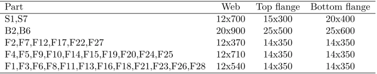
Table 4.2: The crossbeams modeled in Abaqus with notations according to figure 4.4. Units are given in mm.

Part Web Top flange Bottom flange

S1,S7 12x700 15x300 20x400

B2,B6 20x900 25x500 25x600

F2,F7,F12,F17,F22,F27 12x370 14x350 14x350

F4,F5,F9,F10,F14,F15,F19,F20,F24,F25 12x710 14x350 14x350

F1,F3,F6,F8,F11,F13,F16,F18,F21,F23,F26,F28 12x540 14x350 14x350

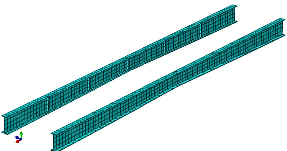
(a) The longitudinal beams and the cross-beams modeled with beam elements with a mesh size of 500mm

(b) The longitudinal beams and the cross-beams modeled with beam elements and with rendered profiles.

(29)

Shell elements

For the main girder between support 5 and 6, where the strain gauges are positioned, and hence the span of biggest influence, shell elements are used instead of beam elements in the finite element model. Contrary to beam elements, shell elements are defined by a surface. Each surface having different numbers of nodes depending on the element used. In Abaqus, diferrent types of shell elements are available. For conventional shell elements, (S4 and S4R), Abaqus uses thick shell theory, Mindlin shell formulation with increasing shell thickness and uses discrete Kirchhoff shell formulation with decreasing shell thickness. The quadrilateral shell element S8R in Abaqus uses a conventional thick shell formulation while the linear shell elements S4 and S4R impose Kirchoff constraints numerically [13].

Mindlin shell elements with full integration are sensitive to locking with decreasing thickness of the elements. The reason for this is that the shear energy term tends to dominate the total potential energy. To avoid this, reduced integration can be used to determine the total potential energy [12]. When connecting the web and flanges, both modelled with shell elements, the possibility of incompatibility exists where the in-plane rotational degrees of freedom of the flange-shell element and the drilling rotational degree of freedom of the web-shell element are shared at the joint. These incompatibilities are however negligible with refined mesh [14].

For detailed and further explanation of the finite element theory, the interested reader can find several books on the subject.

Shell elements, just like 3D beam elements have 6 degrees of freedom in each node, however since the geometrical appearance of the structure is modelled by surfaces and not lines as in beam elements, increasing the mesh will create nodes over the entire surface, hence longer computation time; see Figure 4.6 for the span with the longitudinal beams meshed and modeled as a shell element compared to Figure 4.5a. When assigning a thickness to a shell element it is limited to a surface, however the bridge deck and the longitudinal beams have varying thickness along the span. This is solved by creating partitions on the surface, dividing the surface into sub-surfaces and then assign different thickness properties. Figure 4.7 shows the bridge deck with the partitions in the finite element model and the real bridge deck. The bridge deck and the longitudinal beam in the span of the strain gauges are modelled with shell elements, their numerical values and geometry are presented under section 4.2.

Bridge deck modelled with shell elements

In order to model the correct stiffness of the concrete deck, the shell surface is divided into a total of 39 parts in the longitudinal direction of the deck. This is done, as mentioned earlier to vary the thickness. Each part is assigned with a specific thickness to resemble the tapered shape of the real deck. Table 4.3 presents the numerical values of how the deck is modelled and the partitioning of the deck is shown in figure 4.8.

(30)

X Y Z

Figure 4.6: The longitudinal beams in the span modelled with shell elements and a meshsize of 500mm.

(a) The real appearance of the bridge deck.

X Y

Z

(b) The bridge deck as it is modeled in Abaqus.

Figure 4.7

A short study is done to see how much of an impact increasing divisions have on the strains in the bottom flange, the results are presented in section 6.1.

(31)

Table 4.3: Numerical values of how the deck is modelled . Surface number 1 being the first surface from the edge etc. All values are given in mm.

Surface number Surface width Slab thickness

1 170.0 185.0 2 170.0 355.0 3&39 400.0 420.0 4&38 282.5 179.0 5&37 282.5 197.0 6&36 282.5 215.0 7&35 282.5 233.0 8&34 282.5 251.0 9&33 282.5 269.0 10&32 282.5 287.0 11&31 282.5 305.0 12&30 282.5 323.0 13&29 282.5 341.0 14&28 350.0 350.0 15&27 350.0 350.0 16&26 330.0 343.0 17&25 330.0 329.0 18&24 330.0 315.0 19&23 330.0 301.0 20&22 330.0 287.0 21 3500 280.0

(32)

Main girder modelled with shell elements

The part of the main girder between support 5 and 6 is modelled with shell elements and is divided into a total of eight parts in order to resemble the tapered shape of the beam. Similar to the concrete deck, it is necessary to divide the surfaces into partitions in order to assign different thickness to shell elements created in one part. Figure 4.9 illustrates how this is modelled in Abaqus with respective values.

Position Dimension [mm] 1 1911 2 20 3 42x700 4 47x900 5 20x700 6 38x900 7 47x700 8 50x900 9 18 10 20 11 1792 12 1631 13 1444 14 1635 15 1796 16 1903

Figure 4.9 & Table 4.4: Illustrating how the main girder in span 5-6 is modelled in Abaqus.

(33)

4.3. SUPPORTS AND LOADS 23

4.3 Supports and Loads

Supports

The bridge is modelled as a continuous bridge having 7 supports according to table 4.5. There are three different types of supports along the bridge; roller supports free to move in the x and z directions, roller supports only free to move in the x direction and fixed supports; fixed in all directions. The supports are placed at the bottom flange of the main girder in the real bridge, to model this in the finite element model, a point is created at the bottom flange to which the supports are assigned. This point is then connected to the beam element through a rigid link, see figure 4.11.

Table 4.5: The type of supports and their location along the bridge.

Support number Type of support north side Type of support south side

1 Roller in x, y Roller in x

2 Roller inx, y Roller in x

4 Roller in x Fixed

The north side being the girder following grid D and the south side following grid C according to Figure 4.10.

Figure 4.10: Blueprint showing a plan view of the main girder.

The shape of the supports are neglected in the finite element model since no local effects close to the support are evaluated, only global effects fairly far from the near-est support. Any influence of stress concentrations will have none or insignificant effects on the strains in the bottom flange of the girder. The shape of the supports are shown in figure 4.12.

Loads

Since Abaqaus is a general-purpose software it doesn’t have any built-in functions for moving loads, therefore one must create such functions manually. A script in MATLAB is created for this purpose, where the desired load is moving along a

(34)

defined line over the bridge.

The weight of the lorry is simulated as 6 point loads where the point loads are the loads at the wheels of the lorry as illustrated in Figure 4.13. The lorry geometry is depicted in figure 4.14. Since no local effects are studied in close proximity to the load, but instead the global strains in the bottom flange, the effect of load distribution of the wheels are negligible. The loads are varied in the transverse direction within 5 positions in the right lane. Each position is varied in both the north- and the south direction with 250 mm from the initial position according to Figure 4.15.

Figure 4.11: The supports modelled with a eccentricity in Abaqus.

(35)

4.3. SUPPORTS AND LOADS 25

Figure 4.13: The lorry used for the passing over the bridge [8].

Figure 4.14: Illustration of the lorry geometry [9].

(36)

4.4 Connection and constraints

Since the bridge is modelled with various element types and having composite action between steel and concrete, it needs to follow some conditions/constraints. There are different types of connections in Abaqus, one of the most common one is the Tie Constraint which connects two regions and fuse them together regardless if the regions have dissimilar meshes so that there are no relative motions between them. Two other common connections used in Abaqus are the Coupling Constraint which constrain the motion of a single point on an element to the motion of a surface, and the Spring connection. In the Coupling constrain, the single point is the master and called the control point while the surface is the slave and called the constraint region. A defined influence radius determine the points in the constraint region to be included in the coupling.

Spring connections are used in Abaqus to model springs which connects two regions. They can be modelled as both linear and non linear springs. These connections are described in detail in the following sections.

Main girder

The main girder of the bridge is modeled as a combination of beam elements and shell elements as stated in section 4.2. When assembling the elements, a constraint needs to be assigned in order to connect the two regions. The main girder is con-sidered to be a continuous beam, with two different structural elements and it is for that reason suitable to model a multiple point constraint to connect the two parts. The control point is the end node of the beam elements connected to the edges of the surfaces of the shell elements, see Figure 4.16a. This type of connection is what sometimes in the finite element world is refereed to as a Spider connection, resembling a web of a spider.

The beam elements are however modelled in the same part, sharing the same lines and nodes. This generates a full constraint between the elements. Thus it is not necessary to model further constraints, see Figure 4.16b.

Crossbeams in the span of the Shell Elements

The crossbeams are modeled with beam elements trough out the entire bridge. At the spans where the main girder is modeled with shell elements, a connection needs to be assigned in order to connect the two parts. This is done in the same way as for the connection between the shell elements and the beam elements of the longitudinal beams, using a multiple point constraint connecting the crossbeam to the web stiffener of the longitudinal beam with an influence radius of 250 mm in order to avoid including the nodes at the top and bottom flange in the connection. Figure 4.17 shows an illustration of the connection resembling the bolted connection of the web stiffener.

(37)

4.4. CONNECTION AND CONSTRAINTS 27

X Y

Z

(a) Showing the multiple point constraint con-necting the beam elements to the shell ele-ments of the longitudinal beams.

(b) Beam elements where main girders and crossbeams are modelled in the same part, en-suring full constraint.

Figure 4.16: The constraints between the beam elements and the shell elements of the main girder.

X Y

Z

Figure 4.17: The multiple point constraint between the crossbeams modeled with beam elements and the web stiffener of the longitudinal beam modeled with shell elements with an influence radius of 250 mm.

Interaction of steel- and concrete

The main girder of the bridge is connected to the bridge deck by composite action using studs. The studs and the cross section is depicted in figure 4.18. The com-posite action can be modelled in various ways, but in order to have a fast model, and a model easy to modify its parameters, the connection is modelled with linear axial springs. The springs connect the main girder and the concrete deck which is illustrated in figure 4.19a. They are modelled by using two different approaches;

(38)

Connectors (CONN3D2) which can be seen in figure 4.19b and Engineering Springs (SPRING2).

When using the SPRING2 approach in Abaqus, the springs are modelled in such a way that they are very stiff in the y and z direction so that the only action that is active is the slip action between the steel and concrete, i.e. the stiffness of the spring in the x direction.

The other approach is to use connector elements, CONN3D2, where wires are cre-ated between the mesh-nodes of the bridge deck and the longitudinal beams. The wires are then assigned different properties, having rigid connections in the y and z direction and a defined stiffness in the x direction.

Both methods are modelled by modifying the input file in Abaqus using MAT-LAB. Since the springs are assigned to every mesh-node along the bridge it would be time consuming to do this manually in the CAE, but it is also not possible in Abaqus to assign springs and connections to mesh-nodes in the CAE, only to ver-tices. Therefore by using MATLAB, a script is written in order to assign springs to the mesh-nodes. Rotational springs are not necessary to model since the distance between the linear springs are small enough to avoid any rotational action in be-tween them.

To model and run a simulation resembling full interaction with no slip action, a tied constraint connection is used between the main girder and the surfaces of the bridge deck. To make sure that the two spring-models are working correctly, an influence line for the model with springs is compared to one for the tie constraint model. This is described in detail in 5.1.

(a) Section showing the crossbeam and the two longitudinal beams with their studs, from the blueprints.

(b) A closer look on the longitudinal beams and their studs.

Figure 4.18: The cross section of the main girder.

There are many other ways to model the interaction between the steel and the concrete, but in order to not increase the computation time, since other ways to model the slip action includes non linear behaviours, such as friction, the solution

(39)

4.4. CONNECTION AND CONSTRAINTS 29

with springs is used for this thesis.

(a) Axial springs in theory.

(b) Spring connectors (CONN3D2) assigned to mesh nodes along the bridge deck.

Figure 4.19: The idea of axial springs resembling the slip action between the steel and the concrete in the bridge.

(40)

(41)

Chapter 5

Parametric study

5.1 Parameters

The parameters used in the study are chosen based on the assumption that they will have an influence on the global behaviour of a composite steel-concrete bridge. There are many different types of parameters to study, it is however reasonable to assume that certain parameters have a larger influence on the global behavior than others, this thesis is focusing on the following four;

• The transverse load position. • Young’s modulus for steel. • Young’s modulus for concrete. • Interaction of steel and concrete.

Transverse load positions

The load position in a traffic lane is variable and therefore the different sectional forces which the load gives rise to differs from one load position to another. The bridge model with the current assumptions may be valid for the load placed in a certain load position where certain load effects are more pronounced than others. The deck needs to be modelled with greater detail if the load is placed far away from the main girder since the plate will need to carry the load to the main girders and other effects than global bending may have a great influence in such a case. A varying load position within the right traffic lane is evaluated to study its effect. The choice of traffic lane is based on the assumption that the position of the vehicle only generates global bending of a beam section and other effects such as plate bending and shear lag is negligible. Thus the variation of the load position is fairly close to the main girder.

(42)

32 CHAPTER 5. PARAMETRIC STUDY

Young’s modulus for steel

A large portion of the bridge is made out of steel, therefore the Young’s modulus for the steel might be of great influence. Standards, such as the Eurocode, often have a safety-factor of 1.0 when it comes to steel which indicates that the predicted Young’s modulus for steel often is an accurate value [15]. It doesn’t however have to mean that the predicted value is 100% correct, hence a study to vary the Young’s modulus for steel between 170 GPa and 220 GPa for a predicted value of 210 GPa may have an influence on the global behaviour and therefore of interest to the study. The Poisson’s ratio υ_s is held constant and a value of 0.3 is used for the steel.

Young’s modulus for concrete

Another parameter that is of interest is the Young’s modulus for concrete. The bridge deck is made out of concrete, but for concrete the safety-factor is often set to a value of 1.5 in the standards [16]. This indicates that the predicted value of the Young’s modulus is not assumed to be of high accuracy. Test have shown that the Young’s modulus often is higher on the site than the predicted value stated on the blueprints [17]. Thus a study to vary the predicted value of 32 GPa in a range between 20 GPa and 50 GPa is of interest. The Poisson’s ratio υc is held constant

and a value of 0.25 is used for the concrete.

Interaction between the main girder and the bridge deck

In steel-concrete composite bridges, the interaction between the two are carried out with studs. The slip action between the steel and the concrete has an influence on the global behaviour. The interaction is, as mentioned earlier, modeled with springs, and hence a study varying the spring stiffness constant k in the longitudi-nal, x-direction, is of interest.

The upper and lower limits of k need to be known for the parameter study. This is done by a separate study to see at which value the spring can be considered to be 100 % stiff, i.e. at which value the springs are resembling full interaction between the steel and the concrete. A lower limit for the spring stiffness also need to be determined where the slip action begins to have unreasonable proportions, this is set to be roughly around 20% divergency from the strain range produced by the tie constraint model. To do this, for the SPRING2 connection, a load is applied at a certain node on the concrete deck and the displacements for this node is compared to the associated node in the steel beam. If the displacement between the nodes differ by a reasonably small amount for a certain stiffness, the spring is considered to be 100% stiff. The same is done for the lower value of the spring stiffness where a 20% difference in displacement sets the lower value for the spring stiffness. The springs in the other two directions, y and z, are set to a value high enough to re-semble a fully rigid connection in these directions. This method of using springs did however not reflect the desired behaviour and was therefore rejected as an option

(43)

5.2. MATLAB 33

for modeling the slip action between the steel- and concrete.

For the CONN3D2 model, the value of the connector elasticity for which the influ-ence line reaches full concordance with the tie constraint model is set to the upper value. The lower value is set to a stiffness constant that generate a 20% divergency from the tie constraint model. The connector elasticity in the x-direction is then varied in an interval of 9 different values, while keeping the connector rigid in the y and z direction.

The connector elasticity values are presented in section 6.1.

5.2 MATLAB

In order to do iterative processes, such as writing long input files in Abaqus, MAT-LAB is used. As mentioned in earlier sections, the springs in the model are assigned to every mesh node which results in a large amount of springs. This is done by first understanding how the mesh is created in Abaqus, how the mesh pattern alter with changing geometry and how the pattern is affected by the use of different element types. When this is known, the MATLAB script writes the corresponding section in the input file for assigning springs to each mesh node, assigning springs between nodes on the longitudinal beams and corresponding nodes on the deck being verti-cally aligned to each other. Besides modeling the springs, MATLAB is also used to run the statistical evaluation of the parameters.

5.3 Parametric study and Python scripting in Abaqus

Python scripting

Abaqus uses the programming language Python for scripting and have built-in Python scripts that contain commands to define parameter studies and allows the user to generate, execute and gather the results from the simulations in an effective manner. This is done by creating a parametrized input file containing a parameter definition and a parameter usage, developing a .psf file containing the script which executes the parameter study [13]. The Python script is presented in Appendix A.

Parameter variations

In the statistical evaluation, the simulations must include every possible combina-tion of the varying parameters. The intervals and the number of samples within each interval for the different parameters are presented in table 5.1. The study of the connector elasticity upper and lower limits resulted in the values presented in table 5.1.

(44)

Table 5.1: The samples of the parameter study.

Parameter Number of samples Interval

Young’s modulus for Steel 11 170 - 220 [GPa]

Young’s modulus for Concrete 11 20 - 70 [GPa]

Connector elasticity 9 1e6-1e10 [N/m]

Load position 5 pos.

The simulations are performed with all the possible combinations for the parameters with the load position fixed at one place at a time, five separate input files are created for each load position in the traffic lane which results in 5,445 simulations in total with a total CPU time of 136.125 hours.

5.4 Statistical Evaluation

The statistical evaluation of the results is carried out using the method of Falsifica-tion, which is a scientific method of model updating based on the philosophy that models aren’t fully validated just by observations but can only be falsified. The model updating part of the process is to reach concordance between the predicted results, which is the outcome of the parameter study, and the observed results which are the strains from the the strain gauges. The falsification part is then used to determine which set of parameter values that are accepted [18].

Model updating by the method of falsification

The evaluation of the parameters, using the method of falsification, can be formu-lated as:

g(θi)Cp = yCo (5.1)

where g(θi) is, in the case of this report, the predicted result at the position of the

strain gauge for the n physical parameters θ = [θ1, θ2, ..., θn] and y is the observed

result, the measured strain. The C_p factor is the model uncertainty factor while the Co is a factor considering measurement errors which for electric strain gauges

can be assumed to have a log-normal distribution with unit mean and CoV of 3 percent [19]. The model uncertainty factor, for designing purposes, C_p is set to be a log-normal distribution with a unit mean and CoV of 10% [18]. For the finite element model used in this report, it is however assumed that it will have a lower uncertainty level and is therefore set to a CoV of 3%. If equation 5.1 is rearranged, it can be formulated as:

g(θi)

y = Co

Cp

(5.2) with the quotient of the uncertainty factors being;

(45)

5.4. STATISTICAL EVALUATION 35

Co

Cp

= Cq (5.3)

When C_pand C_oboth are log-normally distributed, its parameters can be calculated as;

λ = λo− λp (5.4)

ζ_q2 = ζ_o2+ ζ_p2 (5.5)

where λ and ζ2 _{are the mean and variance for the logarithm of the random variables,}

respectively. They can be calculated as:

ζ2 = ln(1 + V2) (5.6)

λ = lnµ +1 2ζ

2 _(5.7)

with µ being the mean value and V the coefficient of variation (CoV) [18].

Equation 5.2 shows that the quotient of the predicted and the observed result can be compared to the quotient of the uncertainty factors Cq. The condition is that as

long as the predicting model, i.e. the finite element model, generate results giving a quotient with the measurement equal to Cq, the model instance is accepted. The

relation of the right and the left hand side of equation 5.2 is tested by a conventional hypothesis tests: Ho : g(θi) y = Cq (5.8) and HA: g(θi) y 6= Cq (5.9)

where Ho being the null hypothesis and HAthe alternative hypothesis.

Whether the null hypothesis is rejected or not depends on the statistical distribution and its specified significance level which is for the lower and upper value set to the area corresponding to α/2 in figure 5.1.

(46)

Figure 5.1: Regions of rejection [18].

With α having a significance level between 5 and 10 percent.

The remaining parameters that have not been falsified are the population of values which are capable of reflecting the observed result [18]. The evaluation is performed in MATLAB.

(47)

Chapter 6

Results and discussions

6.1 Model Refinements

Model checking

In order to make the model fast and effective yet accurate enough, several model checks were made which are presented below.

Bridge deck

Since the studied load bearing action of the bridge is global bending, the thickness variation along the deck far away from the main girder is of secondary importance. Only the thickness variation a certain distance away from the main girder could have an influence because a certain part of the deck will undergo global bending together with the main girder. The thickness variation close to the main girder has been studied where a deck with constant thickness equal to the thickness over the flanges, have been compared to the original thickness variation. The result which is shown in figure 6.1 shows that that the strain range difference is negligible, only 2 %.

Crossbeams

The connection between the crossbeams and the web stiffener were studied to see if the rigidity of this connection could have an impact on the global strains. The connection was modelled with rotational springs and the result is presented in figure 6.2 which shows that there is a negligible influence from varying the rigidity of the connection, only 0.8 %.

(48)

38 CHAPTER 6. RESULTS AND DISCUSSIONS Distance/m 0 50 100 150 200 250 300 µ Strain -15 -10 -5 0 5 10 15 20 25

30 Comparison between varying and constant deck thickness

Constant Varying

Figure 6.1: The difference between having constant and varying deck thickness.

Distance/m 0 50 100 150 200 250 300 µ Strain -10 -5 0 5 10 15

20 Influence line showing the effect of rotational springs

1 Nm/rad 1e10 Nm/rad

(49)

6.1. MODEL REFINEMENTS 39

Comparison between the Connector- and Tie constraint model

To ensure that the model with connectors elements is working as desired, a com-parison between a tie constraint model and model with rigid connector elements in all directions was carried out. When the load was placed in the center of the bridge, a difference of only 1.1% is obtained when comparing the strain range for the tie constraint model with the connector model. This ensures that the connector model is working as desired. When the load is getting closer to the longitudinal beams, the difference between the two models increases, to a maximum value of 6.8 % when the load is placed above the main girder. This is because the tie constraint is constraining the whole surface of the top flange which creates a stiffer connection and therefore a lower strain range while the connector only constrains points along the center of the top flange. The comparison of the two models, one with rigid con-nector elements and a tie constraint model, shows that the model with concon-nector elements is valid. Influence lines between the two models, with the two different load positions, are presented in figure 6.3.

(50)

40 CHAPTER 6. RESULTS AND DISCUSSIONS Distance/m 0 50 100 150 200 250 300 µ Strain -10 -5 0 5 10 15 20

Comparison between Tie and Spring model for a moving load placed along centerline of bridge Spring Tie

(a) Difference between the two models with a load placed at the center of the bridge deck.

Distance/m 0 50 100 150 200 250 300 µ Strain -15 -10 -5 0 5 10 15 20 25 30

Comparison between Tie and Spring model for a moving load placed above web of main girder Spring Tie

(b) Difference between the two models with a load placed above the main girder.

(51)

6.1. MODEL REFINEMENTS 41

Time Efficiency

Mesh type

A study of the mesh was carried out where the influence of different mesh sizes were evaluated. The quantity studied was the resulting influence line at the location of the strain gauge. The final mesh and element type were chosen with consideration to the result of the mesh study.

The mesh convergence study was carried out by keeping the mesh density constant in the spans of less influence on the results and varying the mesh in the span of interest. The mesh density in the spans of less influence is the coarsest possible for both the girder beam elements and the deck shell elements, since the mesh density in these spans have no influence on the strains in the span of interest. This was done to save computational time. The mesh density in the span of interest was varied between 500 and 125mm for the girder shell elements and the deck shell elements. The analysis showed that using "S4R5 " elements with a mesh size of .5m and linear interpolation for the shell elements in the span of interest, was sufficient. For the beams in the spans with less influence and the crossbeams in the span of interest, "B31 " element with linear interpolation and the coarsest mesh possible were used. For the deck shell elements in the span with less influence, "S4R5 " elements with linear interpolation and the coarsest mesh possible was used. Influence lines for the different mesh sizes are presented in figure 6.4.

Distance/m 0 50 100 150 200 250 300 µ Strain -15 -10 -5 0 5 10 15 20 25

30 Mesh Convergence for the Tie constraint model

Mesh size: 125mm Mesh size: 250mm Mesh size: 500mm

(52)

42 CHAPTER 6. RESULTS AND DISCUSSIONS

Time step convergence

The influence of the time step had a significant impact on the simulation time, hence a time step convergence analysis was performed and showed that it was sufficient enough with a time step of 5 in order to reach convergence. The resulting influence lines for the different time steps are presented in figure 6.5.

Distance/m 0 50 100 150 200 250 300 µ Strain -15 -10 -5 0 5 10 15 20 25

30 Time step convergence for mesh size 500mm and Tie constraint model

Time step: 1 Time step: 5 Time step: 10

(53)

6.2. STUDIED PARAMETERS 43

6.2 Studied parameters

The outcome from the parameter study and the statistical evaluation indicates that the measured strains can be captured by the finite element model, even for unlikely values of the parameters. This is expected in a composite bridge since the strain distribution over the cross section is dependent upon the relationship between the Young’s modulus of steel and concrete, and the amount of slip which is represented by the connector elasticity. Thus, a low Young’s modulus for the steel in com-bination with a high Young’s modulus for the concrete or vice versa could reach the measured response. The same reasoning is true for the connector elasticity, a more flexible connector produces higher strains than a stiffer one. This would then require lower values of concrete and steel Young’s modulus to reach the measured response.

The parameter study and accompanying statistical evaluation resulted in the follow-ing plots and graphs. Figure 6.6 shows that the behavior of the bridge is described completely by the variation of the input parameters. The x-axis shows the quo-tient between the predicted and the measured response while the y-axis shows the density of parameter combinations that lie within a certain quotient. It seems that the distribution of predicted strains from the finite element model centers around the measured response. The number of parameter combinations that were rejected were 2764 from an original selection of 5445.

0.7 0.8 0.9 1 1.1 1.2 1.3 1.4 1.5 1.6 0 0.05 0.1 0.15 0.2 0.25 0.3 0.35 0.4 g(θ)/y Density All Rejected Uncertainty quotient

(54)

Connector elasticity

The study of the connector elasticity in the longitudinal direction which describes the slip action between the concrete and steel shows that that the elasticity of the connector centers around 1e8 N/m, which can be seen from figure 6.7. This means that the most likely value for the connector elasticity is roughly 1e8 N/m in the bridge model, but all values of the connector elasticity reaches the measured response. The the connector elasticity is here assumed to have a linear relationship between force and displacement, the same need not be true if the connector elasticity is described by a non linear relationship. This is only a representation of the slip-action in the real bridge and is not an explicit value for the real slip resistance in the interface between concrete and steel. The FE model of the bridge requires some elasticity in the connector element to reach the measured response which indicates that there could be some slip action in the real bridge.

1e+06 1e+07 1e+08 1e+09 1e+10

0 0.02 0.04 0.06 0.08 0.1 0.12 0.14 θ 1 = kx/(N/m) Density Initial Updated

Figure 6.7: Initial and updated value for the connector elasticity for all possible combina-tions.

The variation of the connector elasticity seems to have an effect when the values are between 1e7 and 1e9 N/m as can be seen in figure 6.9, which shows the distribution of accepted and rejected strain ranges for all combinations with a certain connector elasticity value, the y-axis shows the quotient between the predicted and measured response. A higher stiffness than 1e9 N/m will not result in any change in strain range. The same is true for stiffness values lower than 1e7. A detailed study of the model uncertainty factor indicates that the connector elasticity is relatively insensitive with respect to the modelling error within a range of 1 to 10 %, this can be seen in figure 6.8a. The same can be said for the measurement error which

(55)

6.2. STUDIED PARAMETERS 45

does not have any effect on the outcome of the results within a range of 3 to 5 % and can be seen in figure 6.8b. Figure 6.8a and 6.8b shows the number of rejected and accepted model instances. The y-axis shows the number of accepted model instances for a certain value of the connector elasticity while the legend shows the total number of rejected model instances with different values of the modelling uncertainty factor in the case of figure 6.8a or the measurement error for figure 6.8b. For these plots, the lowest curve is for a modelling uncertainty factor of 1 % and a measurement error of 3 % respectively and increases upwards.

If the connector elasticity and transverse load position is fixed at 1e10 N/m and at 5 respectively, the distribution curve shifts to the left, see figure 6.10, when compared to figure 6.6, which indicates that the model is to stiff because it generate lower strain ranges for all combinations of parameters.

(56)

46 CHAPTER 6. RESULTS AND DISCUSSIONS 6 6.5 7 7.5 8 8.5 9 9.5 10 200 250 300 350 400 450 500 550 600 Log K x/N/m N reject = 531 N_reject = 742 N reject = 984 N_reject = 1274 N reject = 1602 N_reject = 1971 N reject = 2369 N_reject = 2764 N reject = 3140 N reject = 3386

(a) A detailed study of how the model uncertainty affects the outcome of the result with increasing model uncertainty.

6 6.5 7 7.5 8 8.5 9 9.5 10 250 300 350 400 450 500 Log K x/N/m N_reject = 1969 N reject = 2364 N reject = 2764

(b) A detailed study of how the measurement error affect the outcome of the results with a measurement error range within 5 to 3 %.

(57)

6.2. STUDIED PARAMETERS 47 6 6.5 7 7.5 8 8.5 9 9.5 10 0.7 0.8 0.9 1 1.1 1.2 1.3 1.4 1.5 Log Kx/N/m g( θ)/y Accepted Rejected

Figure 6.9: The accepted and rejected strain range values for all combinations.

0.7 0.8 0.9 1 1.1 1.2 1.3 1.4 0 0.05 0.1 0.15 0.2 0.25 0.3 0.35 g(θ)/y Density All Rejected Uncertainty quotient

Figure 6.10: Distribution of results for all combinations with a fixed connector elactisity of 1e10 N/m and transverse load pos. 5.

(58)

Young’s modulus, concrete

The study of the Young’s modulus for concrete shows, as can be seen from figure 6.11, that the concrete tends to a stiffness value of roughly 55 GPa, but as for the connector elasticity all values of the Young’s modulus of concrete reaches the measured response. The concrete class specified on the blueprints is K40 which corresponds C35/40 according to the damage investigation report from Ramböll [20]. For concrete class C35/40, the Young’s modulus is 32 GPa [16]. The explanation for the higher modulus could be that the concrete delivered to the site may have a higher stiffness than what is specified on the blueprints in combination with the fact that the concrete could have increased its stiffness over time.

10 20 30 40 50 60 70 80 0 0.02 0.04 0.06 0.08 0.1 0.12 θ 2 = Ec/(GPa) Density Initial Updated

Figure 6.11: Initial and updated values for the Young’s modulus of concrete for all possible combinations.

The distribution of strain range decrease with a higher Young’s modulus of concrete as seen in figure 6.13. The reason for this is that increasing Young’s modulus of concrete results in a stiffer cross section, thus lower strains in the steel beams are obtained. As for the connector elasticity, a detailed study of the model uncertainty factor indicates that the Young’s modulus of concrete is relatively insensitive with respect to modelling error. For the finite element model used in this report, the modeling uncertainty is assumed to be between 1 and 5 %. For these values, as can be seen in figure 6.12a, the predicted value of the Young’s modulus of concrete does not change. This shows that the concrete stiffness is relatively insensitive within this range. If however the modeling uncertainty is set to a range within 1 to 10 %, the modulus change from 47-55 GPa. The measurement error does not have any effect on the outcome of the results within a range of 3 to 5 %, seen in figure 6.12b.

Numerical analysis and model updating of a steel-concrete composite bridge: Parametric study & Statistical evaluation