Accelerated dilution of liquefied natural gas plumes with fences and vortex generators: final report, August 1981-May 1982

FINAL REPORT

(August 1981 - May 1982)

prepared by

K. M.

Kothari and R. N. Meroney

Fluid Mechanics and Wind Engineering Program

Department of Civil Engineering

Colorado State University

Fort Collins, Colorado 80523

CER81-82KMK~RNM79

for

GAS RESEARCH INSTITUTE

Contract No. 5014-352-0203

GRI Project Manager

Steve

J. Wiersma

Environment and Safety Department

May 1982

Ul61f0l 0071:.506

J

GRI DISCLAIMER

LEGAL NOTICE This report was prepared by Colorado State University as an account of work sponsored by the Gas Research Institute (GRI). Neither GRI, members of GRI, not any person acting on behalf of either: a. Makes any warranty or representation, expressed or imp 1 i ed with respect to the accuracy, completeness, or usefulness of the information contained in this report, or that the use of any information, apparatus, method or process disclosed in this report may not infringe privately owned rights; or

b. Assumes any 1 iability with respect to the use of, or for damages resulting from the use of, any information, apparatus, method, or process disclosed in this report.

ACCELERATED DILUTION OF LIQUEFIED NATURAL GAS PLUMES WITH FENCES AND VORTEX GENERATORS

1982

..

1. Authof'(s)

K. M. Kothari and R. N. Meroney

~ ··~-

-+-·~-9. Perfomdna Oraanization Name and Address Civil Engineering Department Colorado State University Fort Collins, Colorado 80523

12. Spon<JOnna Orpnlzatfon Name and Addren

Gas Research Institute 8600 West Bryn Mawr Avenue Chicago, Illinois 60613

-15. Supplementary Notes

_______

_. _________ _

352-0203 U. Contntct(C) or Grent(G) No.

(C)

(G)

---+--- -- .

13. Type of Report & Period Covered Final (August 1981 -~---··----'"·--"'·-- t~~2)

14.

1 .. Abstract <Umit: 200 wortts) A wind- tunne 1 test program was conducted on a 1:250 seale model to

determine the effects of fences and vortex generators on the dispersion of LNG plumes. The tests were conducted simulating continuous LNG boiloff rates of 20, 30 and 40 m3J~in; 4, 7, 9 and 12 m/sec wind speed for fence data and 4, 7 and 9 m/sec wind speed for vortex genera-tor data; six configurations; and two heights of fences and vortex generagenera-tors. Plots of ground-level mean concentration contours were constructed. The highest concentrations were observed for the case of no fences and vortex generators. Fences and vortex generators created higher turbulence intensity in the wake and resulted into enhanced mixing thus reducing the ground-level hazards of LNG plumes. In general, the lower wind speed gave the higher ground-level concentration when fence or vortex generator interacted with the LNG plume. However, for the case of no fence or vortex generator the higher concentration per-sisted for longer downwind distances for 7 m/sec wind speed. As expected, the ground-level concentrations were increased with an increase in LNG boiloff rate but decreased with the increase in the fence/vortex generator height. In general, the solid fences gave the lower ground-level concentration as compared with the vortex generator with identical conditions. The double fences or vortex generators gave the maximum LNG plume dilution. However, the single fence or vortex generator near the source gave approximately the same dilution and hence, it would not justify the additional expenses of having second fence or vortex gener-ator. It was also observed that the maximum LNG plume dilution occurs when the fence or

v, .. -erJlQ!<-e€f+ef'~·is-G-ltt5est possible to t..t:t~-NG spill are-a----

---·----1. ...umelt't · An•lyses •· D•.criptors

liquefied Natural Gas, Wind tunnel, Dispersion of heavy plume, Fences, Vortex generators, Turbulent boundary layer.

b. ldantffiers/Open.£nded Terms.

c. COSATI fleld/Grouo

. - - I 21. No. of Paaes 88

---···---,

~~=1~~(Th~

~--! ::o. Security Cl•s• (This Pa•)

~~~~~---·~u~n~c~l~a~s~s~i~f~ie~d~---~~~~~~~=

_{OPTtoHAL FORM 272 (4-77)}

unlimited 22. Price

Sft Instructions on K.,.,..,.,.,

Title Contractor Principal Investigators Report Period Objective Technical Perspective Results RESEARCH SUMMARY

Accelerated Dilution of Liquefied Natural Gas Plumes with Fences and Vortex Generators

Civil Engineering Department Colorado State University

Fort Collins, Colorado 80523

GRI Contract Number: 5014-352-0203

K.

M. Kothari and R. N. Meroney August 1981 - May 1982

Final Report

To determine,, through utilization of wind-tunnel experiments, the effects of fences and vortex gener-ators on the dilution of Liquefied Natural Gas plumes.

A Liquefied Natural Gas (LNG) spill would result in a cold LNG vapor plume, remaining negatively buoyant for a long period of time. The LNG plume could be diluted utilizing passive systems such as a fence or a vortex generator at or near the LNG spill 1

oca-tion. There is a need for determining how these

devices interact with a LNG plume, the optimal sizes and configurations, and the resultant dilution fac-tors a chi evab l e under various wind speeds and LNG boiloff rates.

A large data base on the interaction of LNG plumes with fences and vortex generators was obtained. The wind-tunnel experiments included three simulated LNG

Technical Approach

of fences or vortex generators as accelerating devices for dilution, and two heights for each device. The effects of the variations of these parameters on LNG plume dispersion were obtained. An empirical description of the continuous plume tests was deve 1 oped and advantages of acce 1 erat i ng devices are discussed.

Wind-tunnel tests were performed at a scale of 1:250

to determine the accelerated dispersion of a LNG plume as a result of interaction with fences or vor-tex generators. An LNG plume is heavier than air at boiloff conditions, and is anticipated to remain negatively buoyant for most conditions until it is adequately dispersed. The negatively buoyant plume condition can be simulated in the wind-tunnel by using an isothermal heavy gas of molecular weight equal to that of LNG at boiloff. The measured results should be modified to account for the dif-ference in moles of cold gas vs. the moles in iso-therma 1 gas. The fences and vortex generators of various sizes and shapes were constructed from aluminium plate and heavy gases were introduced into the wind tunnel via an area source of constant diameter mounted flush on the wi nd-tunne 1 floor. The wind tunnel floor was level and smooth for all tests. Gas concentration samples were collected

Project Implications

GRI Project Manager Steve J. Wiersma

downwind of the area source under various

conditions. These samples were analyzed using a gas chromatograph and from this data the plume structure was determined.

This task of the wind-tunnel test program has shown that a passive fence or vortex generator can have a

significant effect on vapor cloud dispersion. They

have excellent promise for practical use in ensuring the necessary di 1 uti on of LNG vapor c 1 ouds in the event of an accidental spill. GRI will use the data obtained to assess the capability of numerical vapor

dispersion models in predicting the functional

relation between spill size, wind speed, fence characteristics, and downwind dispersion distances. The theoretical model and the wind-tunnel results can then be used to design larger-scale tests to

validate wind-tunnel and model results. The end

objective is explicit design guidelines for fences or vortex generators for LNG facilities.

Environment and Safety Department

GRI DISCLAIMER . RESEARCH SUMMARY . LIST OF TABLES . LIST OF FIGURES LIST OF SYMBOLS 1.0 INTRODUCTION . . i i i vi vii X 1

2. 0 MODELING OF PLUME DISPERSION . . . * • • • • • • • • • 4

2.1 PHYSICAL MODELING OF THE ATMOSPHERIC BOUNDARY LAYER . . 5

2.1.1 Partial Simulation of the Atmospheric

Boundary Layer . . . 6

2.2 PHYSICAL MODELING OF LNG PLUME MOTION . . . 8

2.2.1 Partial Simulation of the Plume Motion 9

2.3 MODELING OF PLUME DISPERSION FOR PRESENT STUDY . . . . 15 2.3.1 Physical Modeling of the Atmospheric

Surface layer . . . 15 2.3.2 Physical Modeling of the LNG Spill Plume 16 3.0 DATA AQUISITION AND ANALYSIS . . . .

3.1 WINO-TUNNEL FACILITIES . . . . 3.2 MODEL . . . . 3.3 FLOW VISUALIZATION TECHNIQUES . . . . 3.4 WINO PROFILE AND TURBULENCE MEASUREMENTS 3.5 CONCENTRATION MEASUREMENTS . . . .

3.5.1 Gas Chromatograph . . 3.5.2 Sampling System . 3.5.3 Test Procedure 4.0 TEST PROGRAM . . . .

4.1 Results and Discussion .

4.1.1 Approach Velocities . . .

4.1.2 Flow Visualization Results . . . . 4.1.3 Concentration Measurement Results 5.0 CONCLUSIONS

REFERENCES

APPENDIX A - THE CALCULATION OF MODEL-SCALE FACTORS

v 20 20 20 22 25 28 28 30 31 33 39 39 39 44 81 83 86

Table 1 2 3 4 5 6 7 8 9 10 LIST OF TABLES

Summary of Tests (Fence Data) . . . . Summary of Tests (Vortex Generator Data) . Summary of Plane Area Source Data . . . .

Summary of Fence Data at the Wind Speed of 4 m/sec . Summary of Fence Data at the Wind Speed of 7 m/sec . Summary of Fence Data at the Wind Speed of 9 m/sec . Summary of Fence Data at the Wind Speed of 12 m/sec Summary of Vortex Generator Data at the Wind Speed of

4 m/sec . . . .

Summary of Vortex Generator Data at the Wind Speed of 7 m/ sec . . . · • Summary of Vortex Generator Data at the Wind Speed of 9 m/ sec . . . .

vi

Page 35 36 70 71 72 73 74 75 76 77

Figure

1 Specific Gravity of LNG Vapor - Humid Atmospheric

Mixtures . . . . 2 Variation of Isothermal Plume Behavior from

Equivalent Cold Methane Plume Behavior .

3 Environmental Wind Tunnel

4 5

Model Fences . . . . Model Vortex Generators

6 Velocity Probes and Velocity Standard

7 Velocity Data Reduction Flowchart . . .

8 Photographs of (a) the Gas Sampling System, and (b) the HP Integrator and Chromatograph . . . .

9 Concentration Measurement Locations and

Configuration 0 Identification . . . . 10 Configurations 1 to 3 Identification 11 12 13 14 Configurations 4 to 6 Identification . .

Mean Velocity and Turbulence Intensity Profiles for Equivalent Prototype Wind Speed of 4 m/sec at 10 m Height . . . . Mean Velocity and Turbulence Intensity Profiles for Equivalent Prototype Wind Speed of 7 m/sec at 10 m Height . . . . Mean Velocity and Turbulence Intensity Profiles for Equivalent Prototype Wind Speed of 9 m/sec at 10 m Height . . . .

15 Mean Velocity and Turbulence Intensity Profiles

for Equivalent Prototype Wind Speed of 12 m/sec at

13 18 21 23 24 26 27 29 34 37 38 40 41 42 10 m Height . . . 43 16 Flow visualization (a) No Fence or Vortex Generator;

(b) 4 em (10 m) Height Fence, Configuration 1; (c) 4 em (10 m) Height Vortex Generator, Configuration 4; Equivalent Wind Speed 7 m/sec at 10 m Height,

Equivalent LNG Boiloff rate of 40 m3_{/min . . . . 45}

17 Ground-level Mean Concentration Isopleths

for Run Number 1 . . . 46

Figure Page 18 Ground-level Mean Concentration Isopleths

for Run Number 2 .

. .

.

. .

. .

. . . .

.

.

.

.

47 19 Ground-level Mean Concentration Isopleths

for Run Number 3 .

.

.

.

.

. .

. .

.

.

.

.

48 20 Ground-level Mean Concentration Isopleths

for Run Number 5

.

.

.

. .

.

.

. .

. . .

.

49 21 Ground-level Mean Concentration Isopleths

for Run Number 6 .

. . .

.

.

.

.

.

.

.

.

.

.

.

.

50 22 Ground-level Mean Concentration Isopleths

for Run Number 10

.

.

. .

.

.

. .

.

. .

51

23 Ground-level Mean Concentration Isopleths

for Run Number 14

. .

.

.

. .

.

.

.

.

.

.

.

.

.

.

.

52 24 Ground-level Mean Concentration Isopleths

for Run Number 18 .

.

.

.

.

.

.

.

.

.

.

.

. . .

53 25 Ground-level Mean Concentration Isopleths

for Run Number 19

.

.

.

.

.

54

26 Ground-level Mean Concentration Isopleths

for Run Number 20

. . .

.

. . .

.

.

.

.

.

.

.

.

.

55 27 Ground-level Mean Concentration Isopleths

for Run Number 26

. . .

.

.

.

. .

. .

. . .

.

. . .

.

.

56 28 Ground-level Mean Concentration Isopleths

for Run Number 40

. .

.

. .

.

. .

.

57

29 Ground-level Mean Concentration Isopleths

for Run Number 58

.

.

.

.

. .

. .

.

. . .

58 30 Ground-level Mean Concentration Isopleths

for Run Number 74

.

. .

. .

.

.

.

.

.

. . .

. .

59 31 Ground-level Mean Concentration Isopleths

for Run Number 91

. . . .

.

.

. .

.

. . .

.

60 32 Ground-level Mean Concentration Isopleths

for Run Number 154 .

.

.

. .

.

.

.

.

. .

. .

61 33 Ground-level Mean Concentration Isopleths

for Run Number 169 .

. . .

. .

.

.

.

. . . . .

..

. .

62 34 Ground-level Mean Concentration Isopleths

for Run Number 172 .

.

. .

.

. . .

.

.

. . .

.

.

.

.

63

35 Ground-level Mean Concentration Isopleths

for Run Number 173 .

.

.

. .

.

.

.

.

.

. .

64

36 Ground-level Mean Concentration Isopleths

for Run Number 174 .

.

. . .

. .

.

.

. .

.

. .

. .

65

37 Ground-level Mean· Concentration Isopleths

for Run Number 175 .

. .

.

.

.

.

. .

.

. . .

.

66

38 Ground-level Mean Concentration Isopleths

for Run Number 181 .

. .

. . . . .

. . . .

. . .

.

. . .

67

39 Ground-level Mean Concentration Isopleths

for Run Number 190 .

.

.

.

. . . .

.

. . .

.

.

.

.

. .

68

LIST OF SYMBOLS

Dimensions are given in terms of mass (m), length (L), time (t), moles (n), and temperature (T). Symbol A D g h k L M Ma n p Q T t

u

v

w

X y z Definition Area

Specific heat capacity at constant pressure Molar specific heat capacity at constant pressure

Source diameter

Gravitational acceleration Local plume depth

Thermal conductivity Length

Molecular weight Mach number Mole

Velocity power law exponent Volumetric rate of gas flow Temperature

Temperature difference across some reference layer

Time

Friction velocity Velocity

Volume

Plume vertical velocity General downwind coordinate General lateral coordinate General vertical coordinate

X (L] (Lt- 2] (L] (mLT- 1t- 3] (L] (mn-1] [n] [T] [t) (Lt-1] (Lt -l) [L3] [Lt-1] [L] [L) [L)

Symbol 1\ ilp p a X A p Definition

Surface roughness parameter [L]

Boundary layer thickness [L]

Integral length scale of turbulence [L]

Density difference between source gas and air [mL- 3]

Density [mL-3]

Standard deviation

Mole fraction of gas component

Angular velocity of earth= 0.726 x 10-4 (radians/sec)

Peak wavelength Kinematic viscosity Subscripts and Abbreviations

b.o. Boil off

g Gas

i Cartesian index

LNG Liquefied Natural Gas

m Model NG Natural gas 0 Reference conditions p Prototype s Source gas xi

1.0 INTRODUCTION

Natural gas is a highly desirable form of energy for consumption in

the United States. A sophisticated distribution network already

services a major part of the country. Recen~ efforts to expand this

nation's natural gas supply include the transport of natural gas in a

liquid state from distant gas fields. Also, about 100 peak shaving

plants exist where gas is liquefied during slack periods and vaporized

for distribution during peak use periods. Liquefied Natural Gas (LNG)

is transported and stored at about -162°C. At this temperature if a

storage tank on a ship or land were to rupture and the contents spill out, rapid boiling of the LNG would ensue and the liberation of a poten-tially flammable vapor would result. It is envisioned that if the flow from a rupture in a typical full LNG storage tank could not be con-strained, up to 28 million cubic meters of LNG would be released in 80 minutes [1]. Past studies [1,2] have demonstrated that, for most atmo-spheric conditions the cold LNG vapor plume will remain negatively buoyant until it is adequately dispersed; thus, it represents a ground-level hazard. This hazard will extend downwind until the atmosphere has diluted the LNG vapor below the lower flammability limit (a local con-centration for methane below 5 percent by volume).

It is important that accurate predictive models for LNG vapor cloud physics be developed, so that the associated hazards of transportation

and storage may be evaluated. Various industrial and governmental

agencies have sponsored analytical, empirical, and physical modeling studies to analyze problems associated with the transportation and storage of LNG as we 11 as other 1 i quefi ed gaseous fue 1 s. S i nee these models require assumptions to permit tractable solution, one must perform atmospheric scale tests to verify the accuracy of these models.

A multitask research program has been designed by a combined Gas Research Institute (GRI)/Department of Energy (DOE) effort to address the problem of preditive methods in LNG hazard analysis. One aspect of this program is the physical simulation of LNG vapor dispersion in a meteorological wind tunnel. The complete sub-program research contract,

GRI contract number 5014-352-0203 consists of five tasks.

Task 1: laboratory Support Tests for the Forty Cubic Meter LNG

Spill Series at China lake, California.

Task Physical Simulation in laboratory Wind Tunnels of the

1981 LNG Spill Tests performed at China lake, California.

Task 3: laboratory Simulation of Idealized Spills on Land and

Water.

Task 4: Laboratory Tests Defining LNG Plume Interaction with

Surface Obstacles.

Task 5: laboratory Tests to Determine the Accelerated Dilution

of a LNG Plume by Fences and Vortex Generators near the LNG Source.

Tasks 1 and 2 were presented in the July 1980 and July 1981 annua 1

reports, respectively. Task 2 is also the subject of a final report to

GRI by Neff et a1. (1981) [3].. Task 3 report has been presented by Neff

et al.. [4]. Task 4, the LNG plume interaction with surface obstacles

has been reported by Kothari et al. [5]. Task 5, the accelerated dilu-tion of LNG plume due to fences and vortex generators is the sole subject of this report ..

Some experts currently assume that cons i derab 1 e < mixing takes p 1 ace

during gravity driven vapor spreading; whereas others assume no dilution

3

that models based on such a wide variation of assumptions concerning the kinematics of plume development predict distances to lower Flammability limit (LFL) ranging from fractions to tens of miles for the same spill conditions.

None of the current dispersion mode 1 s incorporate the addi tiona 1 complications of buildings, fences and vortex generators. Such inter-ference may cause additional plume dilution or temporary pooling of high gas concentrations. The purpose of this study was to develop, through the use of atmospheric boundary layer wind tunnels, empirical apprecia-tion of the physics of LNG plume interacapprecia-tion with fences and vortex generators. For fences, four wind speeds, three fence configurations, three LNG boiloff rates, and two fence heights were examined in the wind tunnel. For vortex generators, three wind speeds, three vortex genera-tor configurations, three LNG boiloff rates, and two vortex generagenera-tor heights were examined. Additional tests were conducted without a fence or a vortex generator for three boiloff rates and four wind speeds for comparison with the fence or vortex generator data. The tota 1 of 138

tests were performed during the course of the t'\esearch.

The wind-tunnel test program was conducted on a 1:250 scale model of various configurations. The program consisted of continuous releases of a LNG plume and the subsequent measurement of ground-level concentra-tions up to 500 m scaled downwind distance.

The methods employed in the physical modeling of atmospheric and plume motion are discussed in Chapter 2. The details of model construction and experimental measurements are described in Chapter 3. Chapter 4 discusses the test program and results. Chapter 5 summarizes the conclusions of this research.

2.0 MODELING OF PLUME DISPERSION

To obtain a predictive model for a specific plume dispersion problem one must quantify the pertinent physical variables and param-eters into a logical expression that determines their interrelation-ships. This task is achieved implicitly for processes occurring in the atmospheric boundary layer by the formulation of the equations of con-servation of mass, momentum, and energy. These equations with site and source conditions and associated constituitive relations are highly descriptive of the actual physical interrelationship of the various independent (spill size or spill rate, space and time) and dependent (velocity, temperature, pressure, density, etc.) variables.

These generalized conservation statements subjected to the typical boundary conditions of atmospheric flow are too complex to be solved by

present analytical or numerical techniques. It is also unlikely that

one could create a physical model for which exact similarity exists for all the dependent va~iables over all the scales of motion present in the

atmosphere. Thus, one must resort to various degrees of approximation

to obtain a predictive model. At present, purely analytical or numeri-cal solutions of plume dispersion are unavailable because of the classi-cal problem of turbulent closure [6]. Such techniques rely heavily upon empirical input from observed or physically modeled data. The combined empirical-analytical-numerical solutions have been combined into several

different predictive approaches by Pasquill [7] and others. The

esti-mates of dispersion by these approaches are often crude; hence, they should only be used when the approach and site terrain are uniform and without obstacles such as fences, buildings or vortex generators. Boundary layer wind tunnels are capable of physically modeling plume

5

processes in the atmosphere under certain restrictions. These restrictions are discussed in the next few sections.

2.1 PHYSICAl MODEliNG OF THE ATMOSPHERIC BOUNDARY lAYER

The atmospheric boundary 1 ayer is that portion of the atmosphere extending from ground level to a height of approximately 100 meters within which the major exchanges of mass, momentum, and heat occur. This region of the atmosphere is described mathematically by statements of conservation of mass, momentum, and energy [8]. The general require-ments for laboratory-atmospheric-flow similarity may be obtained by

fractional analysis of these governing equations [9]. This methodology is accomp 1 i shed by sea 1 i ng the pertinent dependent and independent variables and then casting the equations into dimensionless form by dividing by one of the coefficients (the inertial terms in this case). Performing these operations on such dimensional equations yields dimen-sionless parameters commonly known as:

Rossby number Prandtl number Eckert number Pr

=

v 0/(k0/p0CP ) 0 2 . -Ec

=

U 0/Cp (8T)0 0 _ Inertial Force - Viscous.Force _ Inertial Force - Coriolis Force _ Viscous Diffusivity - Thermal Diffusivity

For exact similarity between different flows which are described by the same set of equations, each of thes~ dimensionless parameters must be equal for both flow systems. In addition to this requirement, there must be similarity between the surface-boundary conditions.

Surface-boundary condition similarity requires equivalence of the following features:

a. Surface-roughness distributions,

b. topographic relief, and

c. surface-temperature distribution.

If all the foregoing requirements are met simultaneously, all atmospheric scales of motion ranging from micro to mesoscale could be simulated within the same flow field for a given set of boundary condi-tions [10]. However, all of the requirements cannot be satisfied simul-taneously by existing laboratory facilities; thus, a partial or approxi-mate simulation must be used. This limitation requires that atmospheric simulation for a particular application must be designed to simulate

most accurately those sea 1 es of motion which are of greatest

significance for the given application.

2.1.1 Partial Simulation of the Atmospheric Boundary Layer

A partial simulation is practically realizable only because the kinematics and dynamics of flow systems above a certain minimum Reynolds

number are independent of its magnitude [11,12]. The magnitude of the

minimum Reynolds number will depend upon the geometry of the flow system

being studied. Halitsky [13] reported that for concentration

measure-ments on a cube placed in a near uniform flow field the Reynolds number required for invariance of the concentration distribution over the cube

surface and downwind must exceed 11,000. Because of this invariance,

exact similarity of Reynolds parameter is neglected when physically modeling the atmosphere.

When the flow scale being modeled is small enough such that the turning of the mean wind directions with height is unimportant,

7

simi 1 ari ty of the Ross by number may be re 1 axed. For the case of dispersion of LNG plume near the ground level the Coriolis effect on the plume motion would be extremely small.

2 To

The Eckert number for air is equivalent to 0.4 Ma (~T ) where Ma

0

is the Mach number [6]. For the wind velocities and temperature differ-ences which occur in either the atmosphere or the laboratory flow the Eckert number is very sma 11 ; thus, the effects of energy di ss i pat ion with respect to the convection of energy is negligible for both model and prototype. Eckert number equality is relaxed.

Prandtl number equality is easily obtained since it is dependent on the molecular properties of the working fluid which is air for both model and prototype.

Bulk Richardson number equality may be obtained in special laboratory facilities such as the Meteorological Wind Tunnel at Colorado State University [14].

Quite often during the modeling of a specific flow phenomenon it is sufficient to model only a portion of a boundary layer or a portion of the spectral energy distribution. This relaxation allows more flexibil-ity in the choice of the 1 ength sea 1 e that is to be used in a model study. When this technique is employed it is common to scale the flow by any combination of the following length scales,

o,

the portion of the boundary layer to be simulated; z

0, the aerodynamic roughness; A1, the

integra 1 1 ength sea 1 e of the ve 1 oci ty fluctuations, or .\p, the wavelength at which the peak spectral energy is observed.

Unfortunately many of the sea 1 i ng parameters and characteristic

profiles are difficult to obtain in the atmosphere. They are

be performed. To help 1 ate this problem Counihan (15] has summarized measured values of some of these different parametric descriptions for the atmospheric flow at many fferent and flow conditions.

2.2

PHYSICAL MODELING OF LNG PlUME MOTION

In addition to modeling the turbulent structure of the atmosphere in the vicinity of a test site it is necessary to scale the LNG plume source conditions properly. One approach would be to low the

methodo 1 ogy used in ting the conservation

statements for the combined flow system followed by fractional analysis to find the governing parameters. An ternative approach, the one which will be used here, is that of similitude [9]. The method of similitude obtains scaling parameters by reasoni that the mass ratios, force ratios, energy ratios, and property ratios should be equal for both model and prototype. When one considers the dynamics of gaseous

LNG

plume behavior the following nondimensional parameters of importance are identified [13,14,16, ,18].1'2

Mass Ratio _ _{- effective mass flow of air} mass flow of LNG plume

has been assumed that the dominant mechanism is that of turbulent entrainment. Thus the transfer processes of heat conduction, convection, and radiation are negligible.

2rhe ing of plume Reynolds number is also a significant parameter. Its effects are invariant over a large range making it possible to scale the distribution of mean and turbulent ocities and ax exact parameter equality.

Momentum Ratio

Oensimetric Froude No. (Fr)

Volume Flux Ratio

9

= inertia of LNG plume

effective inertia of air

_ effective inertia of air

- buoyancy of LNG plume

_ volume flow of LNG plume - effective volume flow of air

To obtain simulataneous simulation of these four parameters at a reduced geometric scale it is necessary to maintain equality of the LNG plume specific gravity ps/Pa·

2.2.1 Partial Simulation of LNG Plume Motion

The restriction to an exact variation of the density ratio for the entire life of a plume is difficult to meet for LNG plumes which

simultaneously vary in molecular weight and temperature. To emphasize

this point more clearly, consider the mixing of two volumes of gas, one being the source gas, Vs, the other being ambient air, Va. Consid-eration of the conservation of mass and energy for this system yi e 1 ds

[19]1:

p

.2

v

+

v

pertinent assumption in this derivation is that the gases are ideal and properties are constant.

If the temperature of the air, Ta, equals the temperature of the source gases, Ts, or if the product, CPM, is equal for both source gas and air then the equation reduces to:

(2-8)

Thus for two prototype cases: ·1) an isothermal plume and 2) a thermal plume which is mostly composed of air, it does not matter how one models the density ratio as long as the initial density ratio value is equal for both model and prototype.

For a plume whose temperature, molecular weight, and specific heat are all different from that of the ambient air, i.e., a cold natural gas plume, equality in the variation of the density ratio upon mixing must be relaxed slightly if one is to model utilizing a gas different from that of the prototype. 1 In most situations this deviation from exact similarity is small (see discussion Section 2.3.2).

Scaling of the effects of heat transfer by conduction, convection, or radiation cannot be reproduced when the model source gas and environ-ment are isothermal. Fortunately in a large majority of industrial p 1 umes the effects of heat transfer by conduction, convection, and radiation from the environment are small enough that the plume buoyancy remains essentially unchanged. In the specific case of .a cryogenic liquid spill the influence of heat transfer on cold dense gas dispersion can be divided into two phases. First, the temperature (and hence specific gravity) of the plume at exit from a containment tank and 1If one were to use a gas whose temperature is different from that of the ambient air then consideration of similarity in the scaling of the energy ratios must be considered.

11

surrounding dike area is dependent on the therma 1 di ffus i vi ty of the tank-di ke-spi 11 surface materia 1 s, the vo 1 ume of the tank-dike struc-ture, the actual boiloff rate, and details of the spill surface geome-try. A second p 1 ume phase i nvo 1 ves the heat transfer from the ground surface beyond the spill area into the plume which lowers plume density.

It would be desirable to simulate the entire transient spill phenomenon in the laboratory including spill of cryogenic fluid into the dike, heat transfer from the tank and dike materials to the cryogenic fluid, phase change of the liquid and subsequent downwind dispersal of

cold gas. Unfortunately, the different scaling laws for the conduction

and convection require markedly different time sea 1 es for the various

processes as the length scale changes. Since the volume of dike

material storing sensible heat scales as the cube of length whereas the pertinent surface area sea 1 es as the square of 1 ength heat is trans-ferred to a model cold plume much too rapidly within the model contain-ment structures. This effect is apparently unavoidable since a material having a therma 1 di ffus i vi ty 1 ow enough to compensate for this effect

does not appear to exist. Calculations for the full-scale situation

suggest minimal heating of a cold gas plume by the tank-dike structure thus it may suffice to cool the model tank-dike walls to reduce the heat transfer to a cold model vapor and study the resultant cold plume.

Boyle and Kneebone [19] released room temperature propane and LNG onto a water surface under equivalent conditions. The density of pro-pane at ambient temperatures and methane at -161°C are the same. Using the modified Froude number as a model law they concluded dispersion characteristics were equivalent within experimental error.

A mixture of 50% helium and 50% nitrogen pre-cooled to 115°K was released from model tank-dike systems by Meroney et al. [20], to

simu-late equivalent LNG spill behavior. It was expected the gross

influ-ences of different heat transfer conditions could be determined, however, there was no guarantee that these experiments reproduced quan-titatively similar situations in the field. Since the turbulence char-acteristics of the flow are dominated by roughness, upstream wind profile shape, and stratification one expects the Stanton number in the field will equal that in the model, and heat transfer rates in the two cases should be in proper relation to plume entrainment rates. On the other hand, if temperature differences are such that free convection heat transfer conditions dominate, scaling inequalities may exist; nonetheless, model dispersion rates would be conservative.

Visualization experiments performed with equivalent dense

i sotherma 1 and dense co 1 d p 1 umes revea 1 ed no apparent change in p 1 ume

geometry. Concentration data followed similar trends in both

situa-tions. No significant differentiation appeared between insulated versus

heat conducting ground surfaces or neutra 1 versus stratified approach

flows.

The influence of latent heat release by moisture upon the buoyancy of a plume is a function of the quantity of water

the plume and the humidity of the ambient atmosphere.

vapor present in Such phase change effects on p 1 ume buoyancy can be very pronounced in some prototype situations. Figure 1 displays the variation of specific gravity from a spill of liquefied natural gas in atmospheres of different humidities. For a LNG vapor p 1 ume, humidity effects are thus shown to reduce the extent in space and time of plume buoyancy dominance on plume motion. Hence a dry adiabatic model condition should be conservative.

1.6

,--.---,--..,---,----r----r--r----r---r---.

1.5 :::c: 0 t;;j" (j) 1.4 C\1 @

....

<( ....: 1.3 ..: ~

_I

_{Dry Air} >.

-

>

1.21

0 ~

....

_{75°/o Humidity-}

/ /

<.!)

-t

'""'"" w 0

...

0 1.1 Q) a. (/) I __.. ~ ~ " 100 °/o Humidity I ~ ~~ 1.0 0.90 0.1 0.2 0.3 0.4 0.5 0.6 0.7 0.8 0.9 1.0

Mote Fraction of f·Aethane in Mixture

A reasonably complete simulation may be obtained in some situations

even when a modified density ratio ps/pa is stipulated. The advantage

of such a procedure is demonstrated most c 1 early by the statement of

equality of Froude Numbers.

Solving this equation to find the relationship between model velocity and prototype velocity yields:

where S .. G. is the specific gravity, (ps/pa), and l.S. is the length

scale, (lp/Lm). By increasing the specific gravity of the model gas

compared to that of the prototype gas, for a given length scale, one

increases the reference velocity used in the model. It is difficult to

generate a flow which is similar to that of the atmospheric boundary

layer in a wind tunnel run at very low wind speeds. Thus the effect of

modifying the model specific gravity extends the range of flow

situa-tions which can be mode 1 ed accurately. But unfortunate during such

adjustment of the model gases specific gravity at least two of the fou~_

similarity parameters listed must be neglected. The option as to which two of these parameters to retain, if any, depends upon the physical

situation being modeled. Two of the three possible options are listed

below.

(1) Froude No. Equality

Momentum Ratio Equality

Mass Ratio Inequality

₁

(2) Froude No. Equality

Momentum Ratio Inequality Mass Ratio Inequality Velocity Ratio Equality

15

Both of these schemes have been used to model plume dispersion downwind of an electric power plant complex by Skinner [17], Kothari et al. [21], and Meroney [22] respectively.

The modeling of the plume Reynolds number is relaxed in all phys i ca 1 mode 1 studies. This parameter is thought to be of sma 11

importance s i nee the p 1 ume character wi 11 be dominated by background atmospheric turbulence soon after its emission. But, if one was interested in plume behavior near the source, then steps should be taken to assure that the model plume is fully turbulent.

2.3 MODELING OF PLUME DISPERSION FOR PRESENT STUDY

In the sections above a review of the extent to which wind tunnels can mode 1 LNG p 1 ume dispersion in the atmospheric boundary 1 ayer has been presented. In this section these arguments will be applied to the case of an LNG spill for the present study.

2.3.1 Physical Modeling of the Atmospheric Surface Layer

The neutral boundary layer was generated in the Environmental Wind Tunnel using spires and a trip at the entrance of the tunnel. The wind speeds were referenced to a 10 m (prototype) height. The aerodynamic roughness, z

0, and power law exponent, a, were specified such that the boundary layer profile was similar to that expected for a flat suburban terrain area.

this technique is employed, distortion in velocity scales or similarly volume flow rates requires that a correction be applied to the measured concentration field.

2.3.2 Physical Modeling of the LNG Spill Plume

The buoyancy of a plume resulting from an LNG spill is a function

of both the mole fraction of methane and temperature. If the plume

entrains air adiabatically, then the plume would remain negatively buoyant for its entire lifetime. If the humidity of the atmosphere were high then the buoyancy of the plume will vary from negative to weakly positive. These conclusions are born out in Figure 1, which illustrates the specific gravity of a mixture of methane at boiloff temperature with ambient air and water vapor.

Since the adiabatic plume assumption will yield the most

conservative downwind dispersion estimates this situation was simulated.

Severa 1 investigators have confirmed that the Froude number is the

parameter which governs plume spread rate, trajectory, plume size, and

entrainment during initial dense plume dilution [5,16,19,23,24]. The

modeling of momentum is not of critical importance for a ground source released over a fairly large area. The equality of model and prototype specific gravity was re 1 axed so that a mixture of ethane and carbon dioxide (specific gravity at 1.5) could be used for the model source

gas. The Froude number was maintained at equal values by adjusting

reference wind speed.

The use of an isothermal dense model gas such as mixture of ethane and carbon dioxide in place of a cold methane vapor also results in a slight distortion of the local dynamic forces acting on equivalent plume volumes as the gas mixes. Unfortunately this distortion is not conserv-ative, i.e., the thermal capacitance properties of methane result in plumes which behave more dense than the model equivalent plume. Analy-tical approximations based on the integral entrainment box model of Fay

17

[25] suggest that buoyancy forces are greater at equivalent time and 2

space positions during adiabatic mixing of methane. let Fr = U(h) be

g ~ h

Pa

a local Froude number, where h is local plume depth, U(h) is wind

speed at plume depth, h, and ~p/p is a local density difference ratio.

a

Then given a power law wind profile U(h) ~ ha one finds

Frisotherma1 gas_

{l+xS)(V+(l-~}e)

[ (l+xS+x{l+S)a ]2a [RLNGJ2-4a

FrlNG vapor - (p(1+xS)+(l+S)(l-p)e) (1-xe)(l+xS) Riso

where

x

=

mole fraction methane vapor

R

=

local plume spread

f3 = 1 - M /M _{a s} ~ -0.81 6

=

1- T /T ~ 0.6

s a

S

=

(Cp~/Cp~- 1) ~ 0.22

a= velocity power law exponent~ 0.2.

The variation of this Froude number ratio with equivalent mole fraction methane is plotted in Figure 2. Nonetheless over most of the concentra-t ion range where buoyancy forces are dominanconcentra-t concentra-the variaconcentra-tion of Froude

number is adequately simulated by the isothermal model gas. Indeed,

integral-model calculations when corrected for equal mole source strengths predict equal or slightly higher concentration values at equivalent times.

The actual source condition, i.e., the boiloff rate per unit area

over the time duration of a spill of LNG on land is highly

unpredictable. The source conditions were approximated by assuming a

steady boiloff rate of 20, 30 and 40 m3/min over a constant area.

Since the thermally variable prototype gas was simulated by an isothermal simulation gas, the concentration measurements observed in

,._ 0 0. 0 > (1) c: 0 .c. Q) ::?! ,._ lJ... 3.0 2.5 (/) 0 2.0 (.!) 0 E 1.5 ' -(1) .c.

-

0 _1.0 (/) ,._ lJ... 0.5 0 0 0.2 0.4 0.6 0.8 1.0

Mole Fraction of Methane in Air

Figure 2. Variation of Isothermal Plume Behavior from Equivalent Cold Methane Plume Behavior

19

the model must be adjusted to equivalent concentrations that would be measured in the field. This relationship, which is derived in Appendix A, is:

where

Xm

=

volume or mole fraction measured during the model tests, Ts

=

source temperature of LNG during field conditions,

T

=

ambient air temperature during field conditions, and

a

3.0 DATA AQUISITION ANO ANALYSIS

The methods used to make laboratory measurements and the techniques used to convert these measured quantities to meaningful field-equivalent quantities are discussed in this section. Attention has been drawn to the limitations in the techniques in an attempt to prevent misinterpre-tation or misunderstanding of the results presented in the next section; Some of the methods used are conventional and need little elaboration.

3.1 WINO-TUNNEL FACILITIES

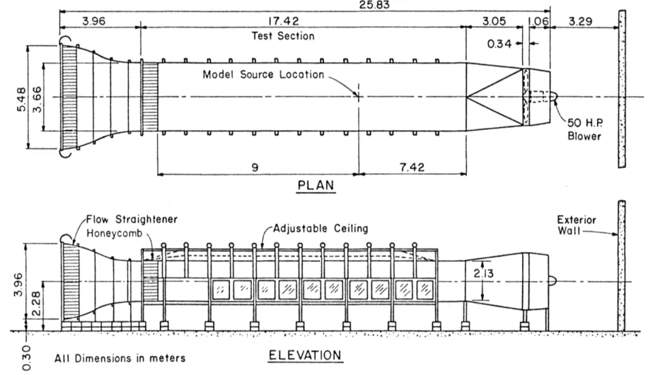
The Environmental Wind Tunnel (EWT) shown in Figure 3 was used for all tests performed. This wind tunnel, specially designed to study atmospheric flow phenomena, incorporates special features such as adjustable ceiling, rotating turntables, transparent boundary walls, and a long test section to permit reproduction of micrometeorological behavior at larger scales. Mean wind speeds of 0.10 to 12 m/s can be obtained in the EWT. A boundary layer depth of 1 m thickness at 6 m downstream of the test entrance can be obtai ned with the use of the vortex generators and trip at the test section entrance and surface roughness on the floor. The flexible test section roof on the EWT is adjustable in height to permit the longitudinal pressure gradient to be set to zero. The vortex generators and trip at the tunnel entrance were fo 11 owed by 8. 8 m of smooth floor for the 1: 250 sea 1 ed area source model.

3.2 MODEL

-Based on the previous atmospheric data obtained at sites similar to that of interest in this study it was decided that the best reproduction of the surface wind characteristics would be at a model scale of 1:250. The area source of a scaled diameter of 75 m was constructed from

3.96 l 17.42 Test Section

T

1

I~

I I I lg§

n _{D D} D D .,

Model Source Location

n D n n ,.

I

~. :

oolw

v<D lrir<") I lt:::::l I I II~ I I ... I.. II I \ 50 H.P.

E

Blower

I

I 7.42

PLAN

~

Flow Straightener Exterior

....---- ,...,, Honeycomb \ (Ad jus to ble Ceiling wo 11 _ _ ::

s:=

~

ili :.:.-

~---

.. -- --- --

~

-- --- -- --

~ ~

F=

~

-

-

-

-

-

r - - - F-=":...tJ..----...--::::r. r== F= 2 13 ~ <D t::= .

9---~ oo ~- . ~ - -

[][?]

1~~ I(/~II~/;II%}{:~11Y~II~ll~/t r - -

1 -

-

-

~·

~ ~~v-'

u

I

.·

~

I I

~

t:=:l l::t J.4

~

J.4 l::t

~

r-i;::,· ~"" ·• " ... •'"'•~-·.,•· .. "~. '" .·.•-'! +···~:·, .. . · ,·•~·'" .. · .. '"'-$ ' • · "~·~· D, . . . • ... _·+~.,-.·~ • • . • :.>:· .. o*··.·~··· .... •.• ., ·· , ... • ... ~·~·,..•;_•'t;.;.~•*'·•· 0 J'()

0 All Dimensions in meters ELEVATION

Figure 3. Environmental Wind Tunnel

N

Plexiglas. The fences and vortex generators were constructed from Aluminium plate of thickness 0.16 em (1/16 in.). The fences had

proto-type equivalent dimensions of 75x75x5 m, 150xl50x5 m, 75x75xl0 m,

150xl50x10 m; and vortex generators had prototype equivalent dimensions

of 75x75x5 m, 150x150x5 m, 75x75x10 m and 150x150xl0 m. The model

fences and vortex generators are di sp 1 ayed in Figures 4 and 5,

respec-tively. The model vortex generators were equilateral triangles with,

1. base 7.6 em, 8 em height, and tilted to the wind flow at 30° such that the tip of the vortex generator as 4 em above ground; the spacing between the vortex generator· was 2.3 em,

2. base 3.8 em, 4 em height, and tilted to the wind flow at 30° such that the tip of the vortex generator was 2 em above ground; the spacing between the vortex generator was 2.1 em.

The source gas, the mixture of 3 percent ethane and 97 percent carbon dioxide, was stored in a high pressured cylinder from which it flowed through a flowmeter and into the circular area source mounted in the wind-tunnel floor.

3.3 FLOW VISUALIZATION TECHNIQUES

Smoke was used to define plume behavior. The smoke was produced by

passing the simulation gas through a container of titanium

tetrachlo-ride. The plume was illuminated with arc-lamp beams. A visible record

was obtained from pictures taken with a Speed Graphic camera utilizing

Polaroid film for immediate examination. Additional color slides were

obtained with a 35 mm camera; and 16 mm silent movie film was taken with a Bolex motion picture camera.

25

3.4 WIND PROFILE AND TURBULENCE MEASUREMENTS

The velocity profile, reference wind speed conditions, and

turbulence were measured with a Thermo-Systems Inc. (lSI) 1050

ane-mometer and a TSI model 1210 hot-film probe. Since the voltage response of these anemometers is nonlinear with respect to velocity, a multi-point calibration of system response ver·sus velocity was utilized for data reduction.

The velocity standard was that depicted in Figure 6. This

consisted of a Matheson model 8116-0154 mass owmeter, a Yellowsprings

thermistor, and a profile conditioning section constructed by the Engineering Research Center shop. The mass flowmeter measures mass flow rate independent of temperature and pressure, the thermistor· measures

the temperature at the exit conditions. The profile conditioning

sec-tion forms a flat velocity profile of very low turbulence at the posi-tion where the probe is to be located. Incorporating a measurement of the ambient atmospheric pressure and a profile correction factor permits the calibration of velocity at the measurement station from 0.1-2.0 m/s.

During calibration of the single film anemometer, the anemometer voltage response values over the velocity range of interest were fit to an expression similar to that of King's law [26] but with a variable exponent. The accuracy of this technique is approximately

the actual longitudinal velocity.

percent of

The velocity sensors were mounted on a vertical traverse and

positioned over the measurement location on the model. The anemometer

responses were fed to a Preston ana 1 og-to-di gi ta 1 converter and then directly to a HP-1000 minicomputer for immediate interpretation. The

HP-1000 computer also controls probe position. A flow chart depicting

"-Compresud Air Figure 6. Screen .... 1• - - t 5 o t3s> •1 r::::::;;:~tt ~=====~ I [0.125 (3.2) Oio. 0.50 02.7}

Hot Film in.(mml

TSI Single Film Sensor

Velocity Probes and Velocity Standard

OiQital Volt Meter

Velocity Sensors

TSI 1050 Anemometers

8 Ch anne I Data Line Input with Buffered Amplifiers

on each Channel

Preston

Analog-to-Digital

Converter

,,

27 Hewlett- Packard HP-1000 Mini-Computer

~

Texas Instruments Line interactive Terminal Printer

Vertical Traverse , r Traverse Control Box Mini- Computer Centro II ed Outputs Control Signal 4~ Disc Storage

3.5 CONCENTRATION MEASUREMENTS

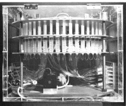
The experimental measurements of concentration were performed using gas-chromatograph and samp 1 i ng systems (Figure 8) designed by Fluid Dynamics and Diffusion Laboratory staff.

3.5.1 Gas Chromatograph

The gas chromatograph with Flame Ionization Detector (FIO) operates on the principle that the electrical conductivity of a gas is directly proportional to the concentration of charged particles within the gas. The ions in this case are formed by the effluent gas being mixed in the FID with hydrogen and then burned in air. The ions and electrons formed

enter an electrode gap and decrease the gap resistance. The resulting

vo 1 tage drop is amp 1 i fi ed by an e 1 ectrometer and fed to the HP 3380 integrator. When no effluent gas is flowing, a carrier gas (nitrogen) flows through the FID. Due to certain impurities in the carrier, some ions and e 1 ect rons are formed ere at i ng a background vo 1 tage or zero shift. When the effluent gas enters the FID, the voltage increase above this zero shift is proportional to the degree of ionization or

correspondingly the amount of tracer gas present. S i nee the

chromatograph1 used in this study features a temperature control on the fl arne and e 1 ectrometer, there is very 1 ow zero drift. In case of any zero drift, the HP 3380, which integrates the effluent peak, a 1 so subtracts out the zero drift.

The lower limit of measurement is imposed by the instrument sensitivity and the background concentration of tracer within the air in

Hewlett Packard 5700 gas chromatograph was used in this study (shown in Figure 6).

29

~)

Figure 8. Photographs of (a) the Gas Sampling System, and (b) the HP Integrator and Chromatograph

the wind tunnel. Background concentrations were measured and subtracted from all data quoted herein.

3.5.2 Sampling System

The tracer gas sampling system consists of a series of fifty 30 cc syringes mounted between two circular aluminum plates. A variable-speed motor raises a third plate, which in turn raises all 50 syringes simul-taneously. A set of check va 1 ves and tubing are connected such that airflow from each tunnel sampling point passes over the top of each designated syringe. When the syringe plunger is raised, a sample from the tunnel is drawn into the syringe container. The sampling procedure consists of flushing (taking and expending a sample) the syringe three times after which the test sample is taken. The draw rate is variable and generally set to be approximately 6 cc/min.

The sampler was periodically calibrated to insure proper function of each of the check valve and tubing assemblies. The sampler intake was connected to short sections of Tygon tubing which led to a sampling manifold. The manifold, in turn, was connected to a gas cylinder having a known concentration of tracer gas. The gas was turned on and a valve on the manifold opened to release the pressure produced in the manifold. The manifold was allowed to flush for about 1 min. Normal sampling procedures were carried out to insure exactly the same procedure as when taking a sample from the tunnel. Each sample was then analyzed for tracer gas concentration. Any sample having an error of greater than

±2 percent indicated a failure in the check valve assembly and the check valve was replaced or the bed syringe was not used for sampling from the tunnel.

31

3.5.3 Test Procedure

The test procedure consisted of: 1) setting the proper tunnel wind

speed, 2) releasing a metered mixture of source gas (specific gravity of 1.5) from the release area source, 3) withdrawing samples of air from the tunnel at the locations designated, and 4) analyzing the samples

with a F 1 arne I on i zat ion Gas Chromatograph ( F I GC). Photographs of the

samp 1 i ng system and gas chromatograph are shown in Figure 8. The

samp 1 es were drawn into each syringe over a 300 s (approximate) time period and consecutively injected into the FIGC.

The procedure for analyzing air samples from the tunnel is as

follows: 1) a 2 cc sample volume which was drawn from the wind tunnel

and collected in syringe is introduced into the Flame Ionization

Detector (FID), 2) the output from the electrometer (in microvolts) is sent to the Hewlett-Packard 3380 Integrator, 3) the output signal is

ana 1 yzed by the HP 3380 to obtain the proportion a 1 amount of

hydro-carbons present in the samp 1 e, 4) the record is integrated, and the

ethane concentration is determined by multiplying the integrated signal

(~v-s) by a calibration factor (ppm/~v-s), 5) a summary of the

integrator analysis (gas retention time and integrated area (~v-s) is

printed out on the integrator at the wind tunne 1 , 6) the integrated

va 1 ues and associ a ted run information were tabula ted on a specially

designed form, 7) the integrated values for each tracer are entered into

a computer a 1 ong with pertinent run parameters, and 8) the computer

program converts the raw data into mean concentration. The calibration

factor was obtained by introducing a known quantity, Xs' of tracer into

The calibration factor is xs(ppm) _{I (J.Jv-s)}

Calibrations were obtained at the beginning and end of each measurement period.

33 4.0 TEST PROGRAM

The goals of the test series were to determine the effects of fences and vortex generators near the source on the dispersion of LNG plume. It is obvious that if one permits variation in source strength, rate of spill, mean flow velocity, fence and vortex generator size, and geometry of separation an almost infinite matrix of tests is possible. However, after discussions with GRI personnel the following test matrix was performed:

1. Continuous LNG spi 11 rates of 20, 30, 40 m3 /min to produce a significant density dominated dispersion region,

2. Four wind speeds, 4, 7, 9 and 12 m/sec at 10 m equivalent

height, for fence data and three wind speeds, 4, 7 and 9 m/sec at 10 m equivalent height, for vortex generator data,

3. Fences and vortex generators of the sizes: 75x75x5 m,

150xl50x5 m, 75x75x10 m, and 150xl50x10 m,

4. LNG boiloff area with diameter of 75 m.

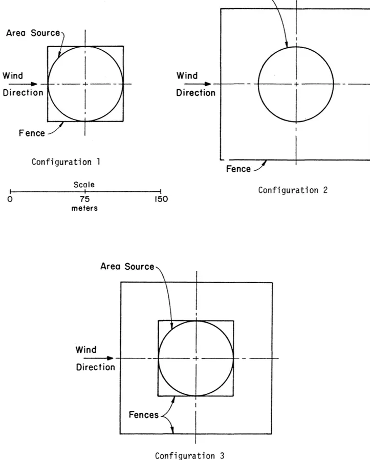
The coordinate system and sampling point locations used throughout this report along with configuration 0 identification, which had no fence or vortex generator, are given in Figure 9. It should be noted that a 11 concentration measurements were performed at ground-1 eve 1. Because of the expected symmetry of the concentration pattern, the sample points were placed only on negative y coordinates. A summary of the test program identifying run numbers, prototype wind speeds, various configuration numbers, fence and vortex generator heights, and LNG boiloff rates is given in Tables 1 and 2. The configurations 1 to 3 and

4 to 6 are described in Figures 10 and 11, respectively. The total

program required 138 runs in the Environmental Wind Tunnel. The follow-ing formulae were utilized to convert field values to model values,

Area Source Diameter I • 2QQ .,, 75.0meters ~, Wind

_{_,...}

1 . Direction Origin of Coordinate System Scale I 1 I 0 75 150 meters 9 17 25

---

-2 10 18. 26 3 II 19 27 4 12 20 28 5 13 21 29 6 14 22 30 7 15 23 31 8 16 24 32

Lateral Distance between Consecutive Sampling Points

=

22.5 meters

Note: All Dimensions in meters

Figure 9. Concentration Measurement Locations and Configuration 0 Identification

w

Table 1. Summary of Tests (fence data)

Fence Fence LNG Wind Run Wind Run Wind

Height Configuration Boil off Speed at Number Speed at Number Speed at

(m) Number Rate 10 m 10 m 10 m

(m3_{/min) (m/sec) (m/sec)}

(m/sec) 0 0 20 4 73 7 1 9 0 0 30 4 74 7 2 9 0 0 40 4 75 7 3 9 5 1 20 4 76 7 10 9 5 2 20 4 77 7 11 9 5 3 20 4 78 7 12 9 10 1 20 4 88 7 22 9 10 2 20 4 89 7 23 9 10 3 20 4 90 7 24 9 5 1 30 4 91 7 18 9 5 2 30 4 92 7 19 9 5 3 30 4 93 7 20 9 10 1 30 4 79 7 14 9 10 2 30 4 80 7 15 9 10 3 30 4 81 7 16 9 5 1 40 4 82 7 26 9 5 2 40 4 83 7 27 9 5 3 40 4 84 7 28 9 10 1 40 4 85 7 30 9 10 2 40 4 86 7 31 9 10 3 40 4 87 7 32 9 Run Wind Number Speed at 10 m (m/sec) 4 12 5 12 6 12 34 12 35 12 36 12 37 12 38 12 39 12 40 12 41 12 42 12 43 12 44 12 45 12 46 12 47 12 48 12 49 12 50 12 51 12 Run Numb en 7 8 9 52 53 54 55 56 57 58 59 60 61 62 63 64 65 66 67 68 69 w ()"'

Fence Fence Height Configuration (m) Number 5 4 5 5 5 6 10 4 10 5 10 6 5 4 5 5 5 6 10 4 10 5 10 6 5 4 5 5 5 6 10 4 10 5 10 6

LNG Wind Run Wind Run Wind Run

Boi 1 o-ff Speed at Number Speed at Number Speed at Number

Rate 10 m 10 m 10 m

(m3_{/min) (m/sec) (m/sec) (m/sec)}

20 4 151 7 169 9 187 20 4 152 7 170 9 188 20 4 153 7 171 9 189 20 4 160 7 178 9 196 20 4 161 7 179 9 197 20 4 162 7 180 9 198 30 4 154 7 172 9 190 30 4 155 7 173 9 191 30 4 156 7 174 9 192 30 4 163 7 181 9 199 30 4 164 7 182 9 200 30 4 165 7 183 9 201 40 4 157 7 175 9 193 40 4 158 7 176 9 194 40 4 159 7 177 9 195 40 4 166 7 184 9 202 40 4 167 7 185 9 203 40 4 168 7 186 9 204 w 0'\

Area Source Wind Oirecf'ion Configuration 1 0 75 meters Wind Area Source - - - . . . . 4 ... J -Oirection 37 Area Source Wind _ _ . .. + -Direction Configuration 2 150 Configuration 3

Wind + -Direction 1 Generator ---1·~ + -Wind Area Source Configuration 4 Direction 0 Scale 75 meters 150 ---1·~ + -Wind Direction Confi gurati n 6 Vortex Generator Configuration 5 Area Source Vortex Generators

39 L = -1- L m L.S. p ' with LNG plume, where, ( S. G. -1 )1/2 (L )1/2 U = m ~ U m S.G. -1 Lp P ' p = (S.G.m-1)1/2 (Lm)5/2 Qm S.G. -1 L Qp ' p p L is 1 ength,

U is reference wind speed at 10 m height, Q is plume flow rate at the source,

L.S. is length scale factor (250),

S.G. is plume specific gravity at the source, and

subscripts m and p indicate model and prototype (field) conditions, respectively.

4.1 RESULTS AND DISCUSSION 4.1.1 Approach Velocities

The approach flow velocity profiles were measured at the location of the area source center. The characteristic mean velocity and turbu-lence profiles are displayed in Figures 12 through 15. The average value of the velocity profile power-law exponent was 0.16. The values of the frictional velocity, u*, were 0.23, 0.42, 0.5, 0.66 m/sec corresponding to prototype wind speeds of 4, 7, 9 and 12 m/sec at 10 m height. The average value of the surface roughness parameter, z

0 for prototype

conditions was 3.8 em.

4.1.2 Flow Visualization Results

The various configurations with vortex generators or fences were installed in the wind tunnel and flow visualization was performed with