Image analysis, an approach to measure grass roots from images

Image analysis,

an approach to measure grass roots from images

(HS-IDA-MD-01-302)

Jonas Hansson

Department of Computer Science

Högskolan i Skövde, PO Box 408

SE-54128 Skövde, SWEDEN

Image analysis,

an approach to measure grass roots from images

Submitted by Jonas Hansson to Högskolan Skövde as a dissertation for the degree of

M.Sc., in the Department of Computer Science.

4/9 2001

I certify that all material in this dissertation which is not my own work has been

identified and that no material is included for which a degree has previously been

conferred on me.

Image analysis,

an approach to measure grass roots from images

Jonas Hansson (a97jonha@ida.his.se)

Abstract

In this project a method to analyse images is presented. The images document the

development of grassroots in a tilled field in order to study the movement of nitrate in

the field. The final aim of the image analysis is to estimate the volume of dead and

living roots in the soil. Since the roots and the soil have a broad and overlapping

range of colours the fundamental problem is to find the roots in the images. Earlier

methods for analysis of root images have used methods based on thresholds to extract

the roots. To use a threshold the pixels of the object must have a unique range of

colours separating them from the colour of the background, this is not the case for the

images in this project. Instead the method uses a neural network to classify the

individual pixels. In this paper a complete method to analyse images is presented and

although the results are far from perfect, the method gives interesting results.

Table of contents

1 Introduction ... 1

2 Background ... 2

2.1 Data ...2

2.2 Other approaches to analyse root images ...3

2.3 Image analysis ...4

2.4 Analysis of the problem ...4

3 Thesis statement ... 7

3.1 Motivation ...7

3.2 Objectives ...7

3.2.1 Preparing data ...8

3.2.2 Adapting a method ...8

3.2.3 Implementation of method ...8

3.2.4 Test of performance ...8

3.2.5 Generalisation ...9

3.2.6 Human interface...9

4 Method... 10

4.1 Using a neural network to identify pixels of dead and living roots...10

4.2 Applying a threshold ...11

4.3 Measuring the identified objects...11

4.4 Filtering out non-root objects ...12

5 Implementation ... 13

5.1 Network input ...13

5.2 Network set-up...14

5.3 Extracting and evaluating objects ...15

6 Results... 17

6.1 Network performance...17

6.2 Extracting and evaluating object...19

7 Analysis and conclusion... 21

8 Discussion and future work ... 23

References ... 24

Appendix C C++ Code... 30

main7.cpp for training, evaluating and using the neural network ...30

tva.cpp used to apply the threshold...40

tre.cpp used for extracting and measuring the thresholded images ...46

image.h a header for handling the images...49

jonas.h a general utility header ...60

vector.h containing a class for storing data about roots...65

1 Introduction

In many fields, both within research and industry, there is a need for image analysis. This

need is often fulfilled by human analysis. There are computerised methods but they often lack

in quality of analysis and, in particular, in flexibility. Many image analysis tasks intend to

measure the shape of objects in the image. In order to do this the objects must first be

identified and extracted from the images. The task of finding objects in an image is easy if it

is possible to use a threshold, for instance if all pixels belonging to objects are lighter than

every other pixel. If it is not possible to find the object with a threshold the task of finding the

objects gets far more complicated.

The images in this project come from a study conducted by the Swedish University of

Agriculture Science. In order to follow the development of grass roots the roots were filmed

from plastic tubes in the soil. The image analysis task is to find the roots in the soil, measure

their size and estimate the volume of the roots. Since the roots as well as the soil vary in

colour the key problem is to identify the roots in the soil; it is not possible to use a threshold.

Instead the images are pre-processed using a neural network before applying a threshold.

From the thresholded images the identified object is measured. Finally the objects are filtered

based on shape and the objects identified as roots are printed out.

This paper first describes the nature of the images to be analysed and gives a general

background to some aspects of image analysis. Next the intentions of this project are

described. Then the method used to analyse the images is presented and the implementation of

the method is described. The reached results are described and analysed. Finally the method is

discussed and ideas for future work are presented.

2 Background

Modern agriculture including modern fertilisers is vital for supplying a growing population

with food. Still, the large amount of fertilisers constitutes a threat to the environment.

Fertilisers leaching from soil to water threaten to turn lakes and bays into sterile wastelands.

One method to minimise this leaching is to grow a catch crop together with the main crop. In

an experiment conducted by the Department of soil sciences at the Swedish University of

Agriculture Science the main crop was spring wheat and the catch crop was perennial rye

grass (Lolium perenne L.). The focus of the experiment was to investigate how the catch crop

affected the movement of nitrate in the soil. In order to investigate the development of the

root systems of the plants, 24 plastic tubes were pushed down the soil and the growth and

decay of the roots were documented using video camera. This documentation was conducted

at six occasions from July 1996 to March 1997. During the documentation the camera could

cover one sixth of the tube’s diameter and stopped to film 24 times while moving upwards.

Thus, the recorded video film, in a sense, consists of stills of the soil and roots. When these

numbers are combined the total number of stills becomes 20 736.

From each of the stills the goal was to analyse the individual roots in the image and measure

its length, diameter and state, where state here simply refers to whether the root is living or

dead. The purpose was to estimate the amount of roots in the soil. Similar analysis has been

conducted manually for similar images from forestry where the roots are large and few. The

images in this case contain many more roots, making the task too laborious to be done

manually. At this stage the department of computer science at University of Skövde was

contacted with the question whether is it possible to perform this analysis with a computerised

mechanism.

2.1 Data

Using the software Media100 the videotapes were converted into RGB images, each with a

height of 576 pixels and a width of 768 pixels. In many of these images the roots are fairly

easy for a human inspector to see as they appear as differently coloured, usually lighter,

ribbons. These images will constitute the input for an analysing system. The desired output

from the system can be thought of as a set of tables, one for each image, where the rows are

the roots and the columns are length, diameter and state, respectively. From these tables the

estimated amount of roots in the soil can easily be calculated.

Even though many of the images are relatively easy to understand for a layman they differ

substantially. The roots differ in width from about 5 pixels for the smaller to about 30 pixels

for the larger. There are differences in the colour of the root and the shape of the roots; some

of them are straight while others have a highly irregular shape. The soil surrounding the roots

differ in colour depending on the soil’s inherit colour and how wet it was at the time of

filming. The texture of the soil also differs with areas of different colour. Finally, the

sharpness of the images differs, see Figure 1.

2.2 Other approaches to analyse root images

One method for computerised measurement of root images it to take up the plants from the

soil, wash them and scan them against a high contrast background. In an experiment

concerning nitrogen absorption by turfgrass, the roots were scanned against a white

background except adventitious roots that, due to their white colour, were scanned against a

black background. The resulting images were then analysed using a Delta-T SCAN image

analysis software (Sullivan et al., 2000). Handling roots in this manner makes the image

analysing task comparatively easy, all the background has one distinct colour and every other

colour is root. The drawback, apart from the work required to create the images, is that the

method is destructive. Since the plants are torn out of the soil it is impossible to follow the

development of individual roots.

The main method for analysing images of roots in soil has relied on humans to mark the roots.

This has been done with and without the use of computers, where the first method involves

tracing the roots with the mouse and the latter uses transparent sheets (Hendrick and Pregitzer

1993; Cheng et al. 1991). One method for computerised analysis of images of roots in soil is

presented by Vamerali et al. (1999). Their method uses the blue band since that band has the

biggest difference in colour between roots and background. The technique applied to the blue

band images in their experiment was first to enhance the contrast of the images. Then they

applied a threshold to the images to produce binary images. From these binary images the root

skeletons were extracted by repeated boundary erosion, basically to remove the outmost

pixels on the major axis of the objects, thus producing one-pixel wide lines representing the

roots. The lines shorter than a defined minimum root length were filtered out resulting in a set

of lines representing the roots. This approach is highly interesting regarding the task in this

paper, however there are differences. In the experiment conducted by Vamerali et al. the

plant, sugarbeets, were planted in lysimeters filled with sandy, clay, silty, loam or organic

soil. As noted by Vamerali et al. the quality of the analysis is influenced by the background’s

colour and homogeneity, they have particular problem with the light sandy soil. The minimum

root length filter improves the analysis, but depending on the definition of the minimum root

These are parts of some of the images. The original images are about six times larger and in full RGB-colour. The first image has three easily identifiable living roots crossing each other in the centre of the image. The second contains dead roots, a wide vertical and a small one lying horizontal over the wider.

The third image contains a young root surrounded by root-hairs. The black object under the root is a stone. The fourth image does not have any roots. An image analysing system should be able to distinguish these objects from root-objects.

length either short roots are filtered out or long non-root-object are classified as roots

(Vamerali et al., 1999). The images in the task presented in this paper differ from the images

used by Vamerali et al. in that they are much more diverse. The soil is from an actual field

with a large amount of object such as stones and old, ploughed in, straws. Also the crop

differs, instead of beets it is species of grass. The impact of these differences is that the

Vamerali et al. method would not give good results for this data, at least not without

significant modifications.

2.3 Image analysis

Any task of extracting data about objects from images can be divided into two subtasks, first

to extract the individual objects and second to measure these objects. (Castleman, 2000). The

first of these subtasks can be thought of as from the original image create a set of images,

each of them representing one object and nothing else. The second subtask is then to measure

these images.

The object locator algorithm uses one of three different segmentation approaches. The first

method is the region approach where each pixel in the original image is classified as

belonging or not belonging to an object. The second approach is the boundary approach where

the aim is to directly identify the boundaries between the regions. The third method, edge

detection, is to first identify the edge pixels and then to link them together to form the

boundaries between objects. This third approach must in its second step be able to distinguish

edges that are boundaries and those that are within objects (Castleman, 2000).

The simplest way to implement the region approach is to use a threshold. If all object pixels

differ in brightness from all background pixels it is possible to apply a threshold to extract the

objects. The correct value of this threshold can be determined using a histogram (Rosandich

1997). A threshold can also work on other values than brightness, such as saturation or degree

of blue in the pixel. Another way to apply the region approach is to use a neural network. The

input to the network is data from the pixel and the desired output is a classification into a set

of classes. By using the network to classify every individual pixel the whole image can be

classified. One interesting advantage of this approach is that is not necessary to define exact

threshold-values, instead the network can be trained on examples (Civco, 1993). To reduce

the impact of noise in the images, Jensen et al used a 3*3 moving window to extract data to be

fed to the network (Jensen et al., 2001).

2.4 Analysis of the problem

The easiest approach to image segmentation is methods that are based on the region approach

by using a threshold. This approach is widely used in image analysis applications. An

example is the MR_RIPL 2.0 program that analyses root images, this program requires that

the roots are lighter than the background. (The MR-RIPL 2.0 user’s guide). For the images in

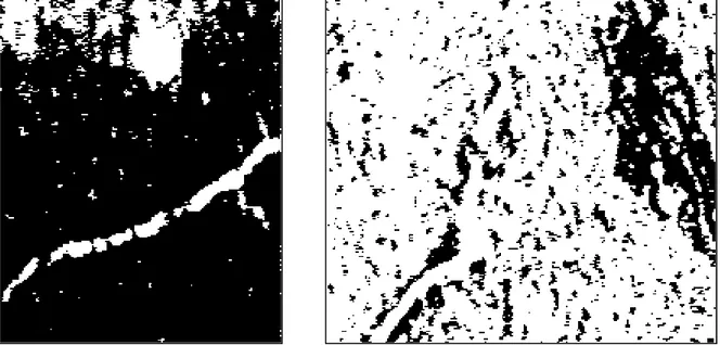
the original image; the problem of different soil colour would increase if the whole image

were thresholded. The threshold value 103 that works well around the root in the left image is

not able to extract the root in the right image in Figure 2. Hence, to use a threshold the best

threshold value must be calculated not only for individual images but the threshold value must

be calculated individual for different parts of the images. The threshold used in figure are

applied on the greyscale level, perhaps better threshold values can be found by if the threshold

values is calculated on the individual colours. But this approach will make the task of finding

the best threshold value much harder. For any RGB encoded pixel there are 16 581 373 (255

-2) possible threshold to consider.

If there is no distinct set of colours that root pixels have and soil pixels do not have, how is it

possible to identify roots? It is impossible to directly identify a root-pixel but it is possible to

identify an area that is on the border between root and soil. In the context here, an edge is a

potential root-edge. An edge is defined as a line along spatial discontinuity (Rosandich 1997)

or less formal; a border area between two colours. Any root is surrounded with edges but the

edges can be surrounding stones or representing the border between wet and dry soil. So edge

is a start but it is not enough to identify the roots.

Even though the roots in the images vary in shape there are some traits of the roots shape that

are shared by the roots and can be used to classify an object as a root. In terms of image

analysis a root can be seen as two long edges stretching over the image. In order to detect

these edges there must be a difference between the colour of the root and the surrounding

image, if there is no difference it is impossible for any system to identify the root.

Furthermore, the edges are lying at a relatively short distance, and this distance is relatively

constant – if the edges do not have these properties they probably surround a non-root object.

Figure 2 Examples of applying threshold.

The left image shows the result of applying the threshold value 103. This value is efficient for extracting the root, however large areas in the upper part of the image also becomes white.

The roots in the images can be classified into two classes, dead and living. Compared to the

task of finding the roots it is relatively hard for a layman to classify a root as dead or living.

Generally, living roots has straighter edges and a smother texture, see Figure 1. Another

feature to help the classification is that dead roots tends to shrink leaving a hole around it, this

can be seen as a dark border around the root. (This can be seen in image 960813-15 in

appendix A).

3 Thesis statement

The background of this thesis is an experiment conducted to analyse root development of

spring wheat and perennial rye grass. This experiment resulted in a large set of images of

roots in soil and the focus of this paper is to investigate computerised methods to analyse

these images. The desired final output from a suitable method is a measurement of the amount

of living and dead root in the soil, i.e. the proportion of the dead and living root mass in the

soil volume. In order to accomplish this, the key problem is to identify the root objects in the

images and to distinguish these objects from irrelevant objects. At the centre of the

investigated method is the use of a neural network to classify individual pixels as belonging to

one of the three classes; living root, dead root or soil.

3.1 Motivation

Many experiments concerning plants produce images of roots in soil. This method to

document natural processes gives good data on how root systems develops. The development

of individual roots over time can be investigated since the documentation does not effect the

root. The basic problem with this approach to document roots is the task of analysing the

images. This task has usually been conducted manually, requiring many and tardy hours.

Methods for computerised analysis of these subterranean images have been proposed.

However these methods usually require that the images have some specific properties, such as

that the roots have a lighter colour than the surrounding soil. Thus, these methods have

problem when confronted with images from field studies. The images in this task come from a

real field so the soil is highly heterogeneous and the roots vary in colour. In addition there are

non-root objects in the soil making the analysis more difficult.

3.2 Objectives

The goal of this master thesis can be decomposed into a number of objectives of varying

importance. The first four in the list presented below are the ones of most importance. In

addition they are, to some degree, in chronological order – it is necessary to choose method

before implementing the method.

• Preparing data

• Adapting a method

• Implementation of method

• Test of performance

• Generalisation

• Human interface

3.2.1 Preparing data

The original data from the department of soil sciences at the Swedish university of agriculture

science was recorded on six videotapes in common VHS-format. These videotapes can be

seen as consisting of a set of stills and these stills must be extracted and stored in a

computerised way. The format of these images should be a format that does not use lossy

compression. Thus formats like TIFF or BMP are appropriate, which to use is a mere practical

matter.

In addition to this video to pixel-image conversion it might be necessary to pre-process the

data to ease the task for the system. Various pre-processing methods could be considered and

these are likely to fall within two categories. One category concerns pre-processing of the

images as a whole, the methods here are likely to be the same as those that would ease any

human inspection of the images. These include methods found in any image-processing

program, like edge enhancement and unsharp mask. The other category concerns

transformations of the individual input sets, for instance, transforming the pixel values from

the standard 0-255 range to a real value ranging between 0 and 1. For each input set these

values will perhaps need to be normalised with respect to brightness. Which pre-processing

methods that will be used depend on the method the system uses and the guidelines found in

the literature concerning this method. The final goal of this step should be to convert the

original video data into data sets suitable for the analysing system.

3.2.2 Adapting a method

Before implementing any image analysing system, it is necessary to choose what method the

system will use. This choice should be based on the literature available about similar

problems. First and foremost this concerns which methods that has been successfully

implemented and, equally important, which that has unsuccessfully been implemented. In

addition, from these successful implementations it is possible to get important clues. These

clues include various hints on how to fine-tune the system, as well as hints on pitfalls to

avoid. The desired output from this step is one method, or a set of methods, likely to be able

to solve the task of analysing the images.

3.2.3 Implementation of method

In order to investigate the adequacy of a potential method it should be implemented. At this

stage the hints and pitfalls identified in the literature plays a vital role. The aim at this stage is

to device a system complete enough to test whether the method chosen can solve the task.

This implies that other features of the system such as its human interface and the speed at

which it process the data are given a low priority.

the system gives any relevant results, or more precise, if it performs better than pure random.

The second is if the system performs good enough. The threshold for this measurement has to

be identified in co-operation with biological expertise.

3.2.5 Generalisation

Having a system that performs well on the set of root images from this field experiment it is

interesting to investigate if the system performs well given another set of images. These other

images could stem from experiments conducted in a different kind of soil and with different

kinds of plants. Is the system able to analyse these images, perhaps with minor modifications?

However, this is not a prioritised objective in this project. Still, the data set presented above is

highly variable with regard to colour and shape of the roots and the colour of the soil and

requires any system to generalise, at least to some degree, in order to solve the task.

3.2.6 Human interface

Having a system that is able to analyse the images, one additional step in this project can be

identified. To enable easy use of the system, the system should be encapsulated with a

user-friendly interface. Even if a user-user-friendly interface is a desirable property this is not a

prioritised property of this project, nor are other software properties such as speed and

memory requirements.

4 Method

As described above the method used by Vamerali et al. (1999) is based on three main steps.

First a threshold is applied to the images so that potential roots become black and the

surrounding soil become white. Next these black objects are skeletonised, reducing them to

1-pixel wide lines. The third step is to filter out root skeletons shorter than a defined minimum

root length (Vamerali et al., 1999).

The method proposed here will be based on the method used by Vamerali et al., but modified

in two ways. First, the roots in this task are not necessarily lighter than the surrounding soil

and consequently, the images must be pre-processed in some manner to produce the binary

black and white images. As Vamerali et al. the segmentation will be based on the region

approach but in a manner that evaluate the individual pixel together with surrounding pixels.

Second the method used by Vamerali et al. filter out non-roots by considering the length of

the skeletons. This is not enough; indeed Vamerali et al. reports problem when there are larger

light objects in the soil.

The method presented here will work in four steps:

1 Using a neural network to identify pixels of dead and living roots.

2 Applying a threshold.

3 Measuring the identified objects.

4 Filtering out non-root objects.

4.1 Using a neural network to identify pixels of dead and living roots

As described above it is not possible to identify a root pixel by just inspecting that individual

pixel; it is necessary to consider a larger part of the image. It would be very hard to exactly

specify what relation a pixel should have to other pixels to be classified as a root pixel. The

method presented here will try to solve this problem by using a neural network. The idea is to

present a backpropagation network with parts of the images and let the network decide if the

pixel in the centre of the input image belongs to a living root, to a dead root or to the

surrounding (Rumelhart et al., 1986). With this approach it is not necessary to manually

define what separates a class of pixel from other classes of pixels, instead the network can be

trained on examples (Civco, 2000).

The size of the input to the neural network should be large enough to give the network the

data needed to make this decision. By presenting the network with every possible image part

of the decided size, every pixel in the image is classified. The only pixels that do not get

classified are those along the edges of the original images. This is because the network only

classifies the pixel in the middle of the input parts. Given that the image parts will be much

where the roots will appear in their assigned colours. Thus this first step can be seen as a

method to transform the image analysis problem to a problem suitable for applying a

threshold.

4.2 Applying a threshold

The output from the first step is images with colours reflecting the network’s confidence in its

classification of the pixels as dead or living roots. In these images the colour-values of the

individual pixels will range from the minimum to the maximum, i.e. from 0 to 255. In order to

extract, measure and evaluate the object the next step is to extract the potential root objects to

distinct objects. All pixel with colour-value above the threshold-value will be set to have the

maximum colour-value, all other pixels will be set to the minimum.

The output from the second step can be seen as two images from each of the original image.

One image where potential living roots appear as black objects and one with potential dead

roots as black objects.

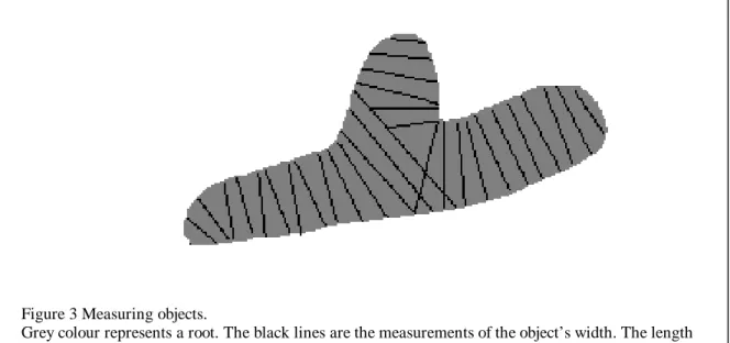
4.3 Measuring the identified objects

The third step intends to measure the shape of the potential roots produced in the earlier steps.

Both the length and the width of the objects should be measured. The length of the objects is,

as in the Vamerali et al. (1999) method, the length of the object’s skeleton. The width of the

objects can be measured by computing how long a line can be drawn within the object if the

line cross the skeleton by 90

°. Since the width of the object vary it is necessary to sample the

width of the object at several points, see Figure 3.

Figure 3 Measuring objects.

Grey colour represents a root. The black lines are the measurements of the object’s width. The length of the object is derived from the number of lines. Notice that a root with a branch is measured as two objects.

4.4 Filtering out non-root objects

The fourth and final step is to use the measurements from step three to filter out irrelevant

objects. As in the method used by Vamerali et al. (1999), objects that are too short should be

filtered out. In addition the intention is to use the measurements of width. Too thick objects

should be filtered out. It is also possible to filter out objects that vary too much in width.

Thus, the final output is a set of measurements of objects classified as root. In this particular

project the desired final output is an estimation of the amount of dead and living root mass in

the soil. This is easily calculated from the length and average width of the objects classified as

roots.

5 Implementation

In order to have an intuitive view of the progress of the system the decision was taken that all

input to the system, and consequently all output from intermediate steps, should be in the

form of images. All parts of the system was coded in C++, see Appendix C. The code was

compiled with a SUN sparc compiler using the command “CC” and executed on a sparc

sun4u.

5.1 Network input

For training and testing the neural network system uses two images in parallel. One of these

images is the unmanipulated image from which the input to the network is extracted. The

second image is a copy of the first on which the roots has been manually marked with red for

living roots and green for dead. From this second image the desired output for the network is

extracted. Thus, the correct classification for the pixel that the network shall classify is found

by looking at the same coordinates in the second image.

From the set of all images, 9 images were selected as train and test images on the basis that

they contained objects of different shape. Copies of the selected images were made. On these

copies the root objects were marked with green for dead and red for living roots. From each of

these marked images a small part containing roots typical for that image was cut out and

saved as a different image, and the same part in the unmarked images was treated in the same

manner. This produced 36 images, two sets with 9 images each for training and two sets with

9 images each for testing. Since the network is intended to classify individual pixels a large

number of train- and test-cases can be extracted from these images.

To further increase the number of input-cases a mechanism to vertically flip half of the inputs

was implemented. The result of this is a huge number of input-cases, too large to process

within reasonable time. In addition, the distribution of the different classes in these

input-cases is highly biased since there are far more soil pixels than there are root pixels. Thus a

method to filter out the bulk of the input cases was implemented. This method counts the

number of pixels in each class that has been fed to the network. Since pixels of dead roots is

least common every such pixel in the training set is fed to the network. Pixels of living roots

is only feed to the network if the number of living pixels already trained on do not exceed the

number of dead pixels already trained on. Pixels of soil are only trained on if the combined

number of dead and living pixels already trained on do not exceed the number of soil pixels

trained on. The consequence of this filtering is that all dead root pixels and most living root

pixels in the training set is used as input to the network. For soil pixels, only a small fraction

of the available pixels are trained on. Since the system processes the image sequentially by

going from left to right, bottom to top, the soil pixels that are trained on lies just to the right of

the roots. To get a more representative distribution of soil pixels to train on the filter for soil

pixels also uses a random function refusing 9 of 10 inputs. This spreads the soil inputs over an

area about ten times as wide as the root. For testing every root pixel is tested, while a filtering

mechanism ensures that soil pixels are only tested if the number of tested soil pixels does not

exceed the combined number of root pixels. Using this methods the network in each epoch is

trained on 60 667 pixels, 15 166 dead, 15 167 living and 30 334 soil and tested on 22 791

pixels, 3 714 dead, 7 681 living and 11 396 soil. Due to the vertical flip of the inputs the total

number of possible inputs for root pixels is twice the number presented above. For soil pixels

the random selection of pixels to train makes the total number of possible training inputs 20

times as big.

The input to the network contains the colour data for red, green and blue of a 29*29 pixel

window. This size is chosen since it enables a whole root to be contained in the window. The

data is converted to a real number ranging from 0 to 1 and these numbers are normalised. In

addition the maximum and minimum value, before normalisation, is fed to the network. This

combined gives 2 525 input nodes.

5.2 Network set-up

The network in this project is based on a backpropagation network originally written by

Karsten Kutza and designed to predict sunspots, see appendix C. This code was changed in

many ways and a large number of settings were tested. As described above the input layer has

2 525 nodes while the output layer has two. The first node in the output layer intends to

classify the pixel as root or soil, giving the output 1 for roots and the output 0 for soil. The

second node in the output layer intends to classify roots into dead or living, giving the output

1 for dead roots and 0 for living, if the pixels is a soil pixels the target for the second node is

0.5.

Since the network’s task is to classify the inputs into discrete classes the exact output is not

important as long as it falls into the correct class, i.e. above 0.5 if the target is 1. Thus a

specialised training was implemented that only backpropagates the error if the absolute error

is more than 0.25 in any of the output-nodes. The benefit of this method is not only to speed

up the process but also to avoid the network’s tendency to favour one specific class.

In every epoch the network is trained on 60 667 pixels and then tested on 22 790 pixels. The

number of epochs the network is trained is not defined in advance, instead the training is

terminated when the network stops improving. To implement this the network-error for the

test cases is measured after every epoch. The measurement selected for this task is the number

of misclassifications in node one, the node that classifies into root and soil. After every epoch

this misclassification ratio is measured. If the error has decreased the weights are saved and a

new epoch is initiated, if the error has not decreased the training is terminated without saving

the weights. Thus, after training the best weight settings found are always the last-but-one and

it is this setting that is saved to be used for classification.

After the training is terminated the network is used to analyse the nine test images. The output

of this usage is fed to a new image of the same size. On this new image the degree of red

shows the network’s confidence in classifying the individual pixels as living root and green as

dead root. In addition, the blue channel is used for the network’s classification as any root.

5.3 Extracting and evaluating objects

The output from the previous step is a set of images where the network has been used to

classify the test-images. On these images the networks confidence in its classification is

reflected in the amount of colour in the individual pixels. The darker a pixel is the more

confident the network is in classifying that pixel as soil, the lighter the pixel is the more

confident the network is in classifying the pixel as a root object. To ease the measurement of

the object the images should be thresholded to create solid objects. Since a pixel can have any

value from 0 to 255 the middlemost value, 127, was used as threshold. The output images

from the previous step are in colour, consisting of red, green and blue. The thresholding is

done individually for each of the three colours. Thus for each of the images the thresholding

can be seen as transforming three greyscale images into three bitmap images there the pixels

either are black or white.

The output from the thresholding can be seen as a set of bitmap images where potential roots

are white and everything else is black. The next step is to measure these objects. The intention

is to measure the width of the objects at several positions. From this the maximum and

average width can be calculated and the length of the objects can be derived from the number

of width measurements.

The first step to measure the objects is to find them. If the images are seen as bitmap images

where pixels belonging to an object are white and all other pixels are black, objects can be

found by traversing the image bottom up, left to right until a white pixel is found. Having

found an object the next step is to find a suitable starting point for the measurements. From

the found white pixel the longest line possible to draw without leaving the white area is found.

Measuring how long it is possible to move in both directions before reaching a black pixel,

repeating this 180 times in every angle and then choosing the longest do this. On this longest

line the middlemost pixel is chosen as starting point for the measurements.

The width of an object at any position is defined to be the shortest line possible to draw that

cross the position and has both its endpoints next to a black pixel, see Figure 3. To stabilise

the process it is necessary to restrict the algorithm to only search for lines that do not differ

from the previous with more than 45

°, thus the algorithm examines the lines in the angles

previous - 45 to previous + 45. For the first width measurement the angle of the previous is

defined to be the angle of the longest possible line (see above) + 90. Having found the first

line, i. e. width measurement, the position where to take the next width measurement has to be

found. This is done in two steps. First the centre point on the found line is calculated and then

the algorithm takes a three pixel step in a straight angle from the found line, i. e. angle of the

found line + 90. By repeating this process the algorithm measure the width of the object at

every third pixel along the object’s length. This is repeated until the end of the object, i. e.

when the next position to make a measurement from is a black pixel. Having reached one end

of the object the process is repeated in the other direction. The starting point for this is second

part is calculated by taking the original starting point and going three pixels in the opposite

direction, i. e. the angle of the longest line + 270. The process of finding the width at every

third pixel is repeated until the second end of the object, by then the whole object is measured.

To avoid measuring the same object over and over again the object has to be filled with

another colour than white. To do this a semicircle is painted behind every width measurement,

the semicircle has a diameter equal to the width and consequently goes from one edge of the

object to the other. The first semicircles lies above the area that the algorithm measures when

the first end is reached and the algorithm starts measuring the second part of the object. This

would mean that this area is not white, and therefor not considered to belonging to an object.

To avoid this the very first semicircle is repainted with white when the first end of the object

is reached. This painting of the object is not complete, small areas along the edge of the object

remains white. But since these areas are short and thin they are removed in the subsequent

filtering. This whole process, finding white pixels, finding starting points and measuring

objects are repeated until the whole image is examined, i. e. when the mechanism for finding

white pixels reaches the upper right corner.

The objects measured in the step above are all white objects in the thresholded images, some

of these objects are proper roots, and some are not. Since proper roots tend to share some

properties regarding their shape it is possible to use these properties to filter out non-roots.

The properties used here are that roots tend to be long and thin both in absolute and relative

values. To enable filtering, three values is calculated for each of the objects: the maximum

width, the average width and the length (length=number of width measurements * 3). Based

on these values four criteria for filtering was used to filter out non-root objects. The exact

settings for these filters were decided experimentally. To be classified as a root the object has

to comply with all of the following criteria:

length >= 15 pixels

average width <= 30 pixels

maximum width <= 50 pixels

length >= 5*average width

The final output after this last step is printed out giving the measurements of the filtered

objects, their length, width sampling, maximum width and average width. Since the specific

aspect that is of most importance to the biologist intended to use the system is the proportion

of root mass in the soil the volume of every root is estimated. This root volume is calculated

based on the simplification that the roots are of cylinder shape so that the volume can be

estimated from the length and average width.

6 Results

In this chapter the results of using the implemented system is described. The main focus in

this chapter is the results of the neural network and of the system as a whole.

6.1 Network performance

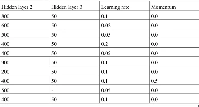
In this project a large number of network settings was evaluated. The network’s performance

was evaluated based on the misclassification ratio in node one; i.e. the share of pixels in the

test set that is missclassified into the classes soil and root. This ratio was calculated separately

for the three classes: soil, dead roots and living roots and the average of these ratios was used

to compare different network settings. This metric was also used as to decide when to

terminate the training as described in section 5.2.

Hidden layer 2

Hidden layer 3

Learning rate

Momentum

800 50 0.1 0.0

600 50 0.02 0.0

500 50 0.05 0.0

400 50 0.2 0.0

400 50 0.05 0.0

300 50 0.1 0.0

200 50 0.1 0.0

400 50 0.1 0.5

500 -

0.05 0.0

400 50 0.1 0.0

The network that performs best of the tested consists of four layers, see Table 1. As described

above the number of nodes in the inputlayer is 2 525 and in the outputlayer 2. The first hidden

layer has 400 nodes and the second hidden layer has 50. The network was trained with a

learning rate of 0.1. The use of momentum decreased the performance so momentum was set

to 0. The performance of this network peaked already in the first epoch. The misclassification

ratio in the first node for this network is 0.2165 for dead roots, 0.2106 for living and 0.2102

for soil. This means that nearly 80% of the pixels are correctly classified into soil and roots.

Compared to the classification in root and non-root pixels the classification of roots into dead

and living give less good results. The misclassification ratio in the second output node is

0.3735 for dead roots and 0.5024 for living, see Table 2.

Table 1. Tested network settings.

For all tested networks the input layer consisted of 2 525 nodes and the outputlayer of 2 nodes. The settings in the lowest row of the table gave the best results and was consequently used to analyse the images.

Pixel class

Misclassification

node one

Misclassification

node two

Average error

node one

Average error

node two

Dead

roots

0.2165 0.3735 0.2567 0.4650

Living

roots

0.2106 0.5024 0.2205 0.4793

Soil 0.2102 -

0.3527 -

After training the network is put to use on the test images. The output of the network for each

pixel is transformed into colour data in the new images. The amount of green in each pixel

represents the networks confidence in classifying the pixels as a dead root, the amount of red

in the pixel represent the classification as a living root and the amount of blue as any root, see

Appendix B. The images created from the network’s output clearly shows the network’s

inability to distinguish between dead and living roots. Especially the green channel,

representing dead roots give strange results with strong output for the edge of roots but low

output at the core of objects, see Figure 4. Thus, the decision was taken to concentrate on the

blue channel, representing roots of any kind. Consequently, the later steps of the method;

thresholding, measurement and filtering, are only conducted on the blue channel and do not

discriminate between dead and living roots.

Table 2. Network performance.

Node one intends to classify pixels into the classes root and soil. Node two intends to classify root pixels into dead and living roots.

The misclassification is the share of the test pixels that is incorrectly classified by the node. Average error is the average absolute difference between desired and actual output.

Figure 4. Network output.

The first part of the image is the input image containing a living root stretching diagonally over the image and a round non-root object above. Next the network output for living roots, dead roots and any roots is shown.

6.2 Extracting and evaluating object

Due to the decision to not distinguish between dead and living roots the output from the

network-part of the system can be seen as nine greyscale images. The pixel-value of the

individual pixel, i.e. their brightness, represents the network’s confidence in classifying that

pixel as belonging to a root. The next step of the method is to apply a threshold to the images.

The perfect output for node one is 0 when classifying a soil pixel and 1 when classifying a

root pixel, represented as 0 and 255, respectively, on the output images. Thus, the middlemost

value, 127, was chosen as threshold value. Any pixel with a lower pixel value is set to black,

every other pixels is set to white.

The result of applying the threshold can bee seen in Figure 5 as the difference between the

second and third section of the images. All white objects in the third sections of the images

are potential root objects, some are proper roots and some are misclassifications. The next

step is to measure these objects as described in section 5.3. When the objects are measured the

system gets a large numbers of arrays describing the object as a number of width

measurements where the length of the objects can be derived from the number of widths. The

last step of the method presented here is to filter these arrays to remove objects whose shape

does not resemble that of a root. The arrays that remains after filtering are presented to the

screen. The data presented are x and y giving the starting point of the object, where the

co-ordinates 0, 0 is the lower right corner. Next a number of measurements of the object is

presented: length, maximum width, average width and an estimation of the volume of the

object. And finally the width measurements are printed. The units in these measurements are

number of pixels or cubic pixels. For the image 960905-15 the printout is:

Vector 74 14 62 12 8.225806 3294.871973

4 5 7 8 10 10 9 10 10 10 9 10 11 12 12 9 8 8 11 11 9 7 5 4 4 6 8 10 10 7 1 Vector 127 41 56 14 9.750000 4181.067123

12 12 12 13 14 14 13 13 11 10 10 10 10 8 7 6 7 5 4 4 3 12 12 11 12 13 9 6

As described in section 5.3 the algorithm that measures the object fills the object it measures

by painting semicircles behind every width measurement. The implementation of the

algorithm changes the colour of the semicircles for every new object giving every object its

unique colour. With the help of these unique colours and the co-ordinates printed to the screen

it is possible to manually edit the output images from the system so that only the objects that

Figure 5. Results

This image shows the output from different steps of the method. The first part is the original input image. Next the image created by the neural network showing the network classification as root. The third part is the result of applying the threshold. The fourth part is the results after filtering; showing the object the system classifies as roots.

the system consider to be roots remains. This editing is not a part of the method; it is only

done in order to evaluate the results. Since the filling of the object only is intended to prevent

the same object from being measured over and over again the shape of the filled object is not

exactly the same as that of the original object. This difference in shape can be seen when

comparing the third and fourth sections of the image in Figure 5. The third section is the

output after threshold and the fourth is the final, manually edited, image representing the

object the system consider to be roots.

The imperfection in the filling of the objects must be kept in mind when analysing the final

output of the system. The actual results, presented as the screen-output above, are somewhat

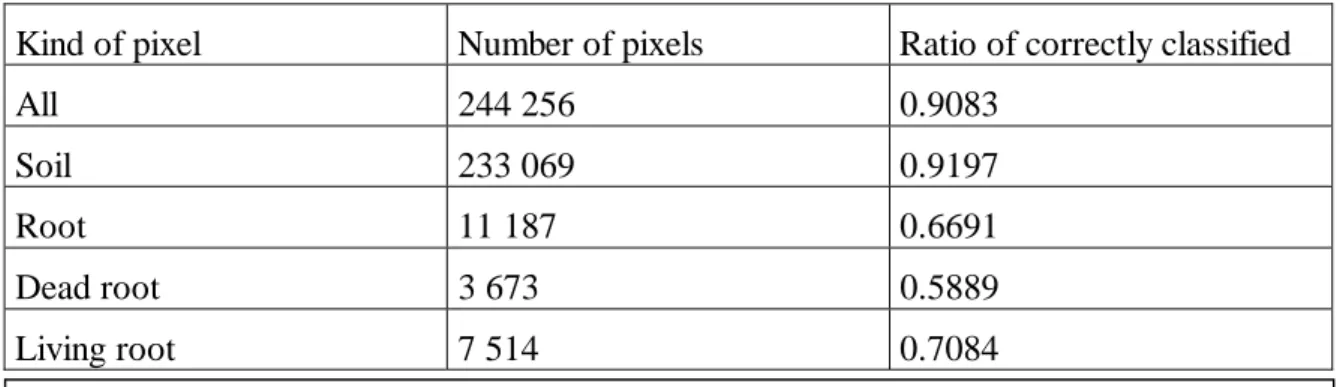
better than what the images in Figure 5 and Appendix A imply. The images of the final output

can also be used to measure the results on a pixel-by-pixel level. By comparing each

individual pixel of the images used as target for the network and the final output images the

share of pixels that is correctly classified can be estimated, these results are presented in Table

3.

Kind of pixel

Number of pixels

Ratio of correctly classified

All 244

256

0.9083

Soil 233

069

0.9197

Root 11

187

0.6691

Dead root

3 673

0.5889

Living root

7 514

0.7084

Table 3 final results.

7 Analysis and conclusion

Given the nature of the images in this task, no system can perfectly analyse them. The high

resolution and the imperfect sharpness of the images make it impossible to exactly pinpoint

the border of root objects. And even if the resolution would be lower and the sharpness

perfect there would be borderline cases with pixels lying just over the border between root

and soil. Also the distinction between living and dead roots have borderline cases. As a root

dies it slowly change its appearance from that of a living root to that of a dead. Thus, no

system can exactly classify a root as dead or living. This lack of perfection must be kept in

mind when evaluating the system designed in this project. The results presented above

compare the system output to a target output. This target output is derived from a set of

images where the root objects are marked manually. These images can not be considered the

absolute truth, the exact border of the marked objects is an approximation and there might be

misclassification of entire objects. However, the target images are created in co-operation

with biological expertise and are exact enough for the purpose here.

The results can be divided into two categories, the system’s ability to find roots of any kind

and secondly the system’s ability to classify these roots into dead and living. The results for

the first category are relatively good. The network’s ability to distinguish root pixels from soil

pixels reaches almost 80% correct classification. This is far beyond pure random and in the

images of network output the roots are generally visible as lighter objects, see Figure 5. The

later filtering step of the method can not identify root objects not found by the network but it

can remove non-root object. Also this step is relatively accurate. The filtering is done

perfectly in image 960905-15 and 961007-22. For other images, such as image 960813-15,

both root objects and non-root objects are removed.

While the system performs relatively well on the task of identifying the root object, the

performance concerning classification of roots into dead and living works less well. The

network is able to correctly classify 63% of the dead pixels and 49% of the living. Of all root

pixels 54% are correctly classified into dead and living so the network seems to have some

ability to distinguish between dead and living. But the margin over pure random is just 4

percentage points and this is far below what necessary for a useful system. Consequently, the

later steps of the method concentrated on root objects of any kind, rather than to separate them

into dead and living.

These differences in results between finding and classifying roots are not surprising. A human

inspector has relatively small problems finding the roots but to tell if they are dead or living is

much harder. Even experts have problems making the distinction.

In Chapter 3.2.4, Test of performance, two measurements were defined. The first was whether

the system performed above pure random and the second was if the system performed good

enough to be useful. For the task of classifying the roots into dead and living the system can

be considered to perform just, but only just, above random. Given the mediocre results the

second measurement of usability must be considered not fulfilled. For the task of identifying

roots of any kind the results are better. The system performs far better than pure random so

the first measurement is passed with good margin. The measurement of usefulness must be

considered with respect to alternative methods, in this case manual analysis of the images.

This manual inspection is not only very expensive but the accuracy of the analysis is not

perfect. This imperfection comes from problem associated with analysis of the images,

described in the first paragraph of this chapter. In addition, the field study that the images in

this task stems from produced 20 736 images. Human analysis of such a huge number of

images is bound to encounter human errors. Keeping this in mind the task of finding and

measuring roots can be considered to be fulfilled since the department of soil sciences at the

Swedish university of agriculture science intends to use the system designed in this project to

analyse the images.

8 Discussion and future work

The system implemented in this project is intended to test the principles of the method. It is

likely that far better performance can be reached if the system is properly fine-tuned. In

particular, the neural network step can probably be further improved. The architecture and

settings for the network can be further improved. Perhaps backpropagation is not the best kind

of network paradigm for this task. Since the network is intended to classify high dimensional

data it would be interesting to use a self-organising map (Kohonen, 1988). The performance

of the network can perhaps be improved by pre-processing the input. The current system uses

RGB-colours as input. Another encoding of colour images is HSB that represent colour using

its hue, saturation and brightness. Compared to RGB, HSB-encoding is closer to how humans

perceive colours and perhaps the network will find such encoding easier to interpret (Russ,

1992). Also the choice of training inputs can be improved. Since there are far more soil pixels

than root pixels the system selects a subset of the soil pixels randomly. By inspecting the

output image from the network it might be possible to find types of soil pixels that the system

tends to misclassify. With this information it would be possible to make a more informed

selection of soil pixels to train.

Since the current system only intends to test the method some issues has to be addressed in

order to transform it into a proper application. It must be equipped with a user interface

allowing easy use of the system. In addition, the current system would take approximately one

hour to analyse one complete image; this time should be decreased. As any program this can

be achieved by optimising the code. Another way to speed up the system is to decrease the

resolution of the images. If the images are transformed such that each square of four pixels are

combined into one pixel the network input is decreased with a factor four, assuming that the

input cover the same area in the image. The impact on time is obvious, the impact on the

quality of classification is harder to predict. The quality might decrease since the network

simply gets less data. But the quality might increase since the network gets a less noisy, less

chaotic data.

The system implemented in this project is intended to measure roots. However, the high level

method is not restricted to just roots, it might be possible to use the method for other image

analysis projects. The results for classification of roots into dead and living imply that the

method has its limitations but there might still be other domains there the method will produce

usable results, possibly better than for the roots in this project.

References

Castleman K.R., Image analysis: quantitative interpretation of chromosome images. Image

processing and analysis. eds Baldock R., Graham J. Oxford university press, New York, USA,

2000.

Cheng W., Coleman D. C., Box Jr J. E., Measuring root turnover using the minirhizotron

technique. Agriculture ecosystem environment 34:261-267 1991.

Civco Daniel L., Artificial neural networks for land-cover classification and mapping.

International journal for geographical information systems vol. 7 No. 2 173-186, 1993.

Hendrick R. L., Pregitzer K. S., Patterns of fine root mortality in two sugar maple forest.

Nature 361:59-61 1993.

Jensen R. J., Qiu F., Patterson K., A neural network image interpretation system to extract

rural and urban land use and land cover information from remote sensor data. Geocarto

international vol. 16 No. 1. March 2001.

Kohonen Tuevo, The neural phonetic typewriter 1988, I Patternrecognition by selforganizing

neural networks editerad av Carpenter Gail A. och Grossberg Stephen, Bradford book,

Cambridge

Rosandich R. G., Intelligent visual inspection using artificial neural networks. Chapman &

Hall, Padstow, UK, 1997.

Rumelhart D. E, Hinton G. E, Williams R. J., 1986 Learning Internal Representations by

Error Propagation. Parallel Distributed Processing, Volume 1 MIT Press, Cambridge, MA, pp.

318-362, 1986

Russ John C., The image processing handbook. CRC Press, Boca Raton, Florida, 1992.

Sullivan W., Jiang Z., Hull R. J., Root morphology and its relation with nitrate uptake in

kentucky bluegrass. Crop Science 40:756-772 2000.

http://rootimag.css.msu.edu/MR-RIPL/MR-Appendix A

Images from different steps of the algorithm.

All the images shows first the test image (originally in full RGB-colours), then the networks

output for the blue channel, then the result of applying the threshold value 127 and finally the

result after filtering. The number refers to the date when the image was taken and the depth

(the date in Swedish format: YYMMDD).

960703-27, living root.

The system gives relatively good results in this case. Only a small non-root object remains

after the final step.

960813-15, dead root

The input image contains one root going vertical in the right side of the image. The final

image shows that the system only recognise parts of the proper image together with some

non-root objects.

960905-15, dead root

This is the same root as in the image above but the picture is take almost one month later. The

system performs very well in this case.

960905-26, living root

The root goes diagonal across over the image, the round object above is not a root. Apart from

a small object at the bottom of the image the system is able to find the correct object.

961007-11, dead root

In the input a small root is going horizontal over the image. The system is not able to identify

the root.

970321-09, living root

In this case a root is going diagonal in the right part of the input. The system identifies that

root together with some none-root objects.

961007-07, living root

The input contains one young root with root-hairs going vertical over the image and a black

stone. The systems performance can only be considered as a complete failure on all accounts.

961007-22, dead roots

The input contains one horizontal root in the upper part of the image and one vertical in the

lower part. The output from the network recognises these roots together with a large number

of non-root objects. After filtering only the correct objects remain.

Appendix B

Histograms

Histograms showing the colour-distribution in the images produced by the network. X-axis

shows the colour-value, y-axis the proportion of pixels. The histograms to the left is

calculated on the pixels that should have the colour, the histograms to the right is calculated

on the pixels that should not.

0 0,05 0,1 0,15 0,2 0,25 0,3 1 26 51 76 101 126 151 176 201 226 251 Blue roots 0 0,02 0,04 0,06 0,08 0,1 0,12 0,14 0,16 1 26 51 76 101 126 151 176 201 226 251 Blue soil 0 0,02 0,04 0,06 0,08 0,1 0,12 1 27 53 79 105 131 157 183 209 235 Red living 0 0,02 0,04 0,06 0,08 0,1 0,12 0,14 0,16 1 26 51 76 101 126 151 176 201 226 251 Red not living

0 0,005 0,01 0,015 0,02 0,025 0,03 1 27 53 79 105 131 157 183 209 235 Green dead 0 0,02 0,04 0,06 0,08 0,1 0,12 0,14 0,16 1 26 51 76 101 126 151 176 201 226 251 Green not dead

Appendix C

C++ Code

main7.cpp for training, evaluating and using the neural network

{printf("\nloggFlush the logg file is impossible to open \n"); exit (1);

} }

void trainDriver(BPbox &net, Arr<imageHandler> &trainFa, Arr<imageHandler> &trainIn, ulong ix, ulong iy)

{ulong i, xe, ye, fdead=0, fliving=0, fsoil=0, x, y, turns=0; imageHandler ipart;

double dead, living;

double dr=0, dk=0, lr=0, lk=0, sr=0, sk=0; //Diffs, exept the (irrelevant) sk that is average

Arr<double> input; Arr<double> output; Arr<double> facit(2); int flipp;

for (i=0; i<trainFa.gelangd(); i++) {

if (! (( (trainFa[i].getWidth()==trainIn[i].getWidth()) &&

(trainFa[i].getHeigth()==trainIn[i].getHeigth()) ))) {printf("bonusDriver() the two images in set %d was of different size", i); exit(1);};

//The outer limits of the input-taking xe=trainFa[i].getWidth()-ix; ye=trainFa[i].getHeigth()-iy; x=0; y=0; printf("\n"); while (y<ye+1) { flipp=rand() % 2;

} else {

if (trainFa[i].isColour(x+ix/2, y+iy/2, 0, 255, 0)) dead=1; else dead=0;

if (trainFa[i].isColour(x+ix/2, y+iy/2, 255, 0, 0)) living=1; else living=0;

}

/*This condition is to ensure that, in the long run, there's equal amount of the differents cases.

The assumption is that soid is more common than living which is more common than dead.

I've changed it since it got too few soils from living images. */

if ((dead==1) || ((living==1) && (fdead >= fliving)) || (((dead==0) && (living==0)) && (fdead+fliving >= fsoil)))

{

turns=turns+1;

if (dead==1) fdead=fdead+1;

else if (living==1) fliving=fliving+1; else fsoil=fsoil+1;

trainIn[i].imagePart(ipart, x, y, ix, iy, 0); if (flipp) trainIn[i].VFlipp();

ipart.toDouble(input);

//Node one - root or not. Node two what kind of root. Thus: r-node and k-node if (dead > 0.5) //Deads { facit[0]=1; facit[1]=1; }

else if (living > 0.5) //Living { facit[0]=1; facit[1]=0; } else //Soils { facit[0]=0; facit[1]=0.5; }

net.train(output, 1, 1, input, facit);

if (dead > 0.5) {dr=dr + output[0]); dk=dk + abs(1-output[1]);}

else if (living > 0.5) {lr=lr + abs(1-output[0]); lk=lk + output[1];} else {sr=sr + output[0]; sk=sk + output[1];}

imageHandler fbild; double d,l;

trainFa[i].imagePart(fbild, x, y, ix, iy, 0); if (flipp) fbild.VFlipp(); if (fbild.isColour(ix/2, iy/2, 0, 255, 0)) d=1; else d=0; if (fbild.isColour(ix/2, iy/2, 255, 0, 0)) l=1; else l=0; if ((d != dead) || (l != living)) {