Research
2010:05
Discrete-Feature Model Implementation
of SDM-Site Forsmark
Title: Discrete-Feature Model Implementation of SDM-Site Forsmark Report number: 2010:05
Author: Joel Geier, Clearwater Hardrock Consulting, Corvallis, U.S.A.
Date: Mars 2010
This report concerns a study which has been conducted for the Swedish Radiation Safety Authority, SSM. The conclusions and viewpoints pre-sented in the report are those of the author/authors and do not neces-sarily coincide with those of the SSM.
SSM Perspective
SSM has been following the investigations of the two candidate sites for a repository for spent nuclear fuel that the Swedish Nuclear Fuel and Waste Management Company (SKB) have been undertaking. SKB has reported the results of the investigations as site descriptive models. These models will be used to underpin the safety analysis following the license applica-tion of the repository planned by SKB. One important aspect in the safety analysis is the water flow to, around, and from the repository. In order to model these, discrete fracture network (DFN) models can be used. Such models can capture the stochastic nature and complexity of the hydrolo-geologic situation at a site. SSM has funded Clearwater Hardrock Consult-ing to investigate flow around the planned repository in Forsmark usConsult-ing a DFN model especially designed for this task. In addition, deposition hole utilisation factors have been quantified. The results are considered to be useful for SSM as independent estimates that may be compared to SKB’s results in the up-coming license application. Moreover, the results can be used as a baseline for comparisons to other model variants or alternative models that may be investigated.
Results
A discrete-feature model (DFM) was implemented for the Forsmark repository site based on the final site descriptive model from surface-based investigations. The DFM model appears to be practical with a modelling cycle of about two weeks per realization.
An improvement in deposition hole utilization factors of 10% to 15% relative to the previous Forsmark DFM model was obtained. This is closer to SKB’s results in SR-Can (SKB, 2006), and is believed to be a result of an improved DFN generation algorithm that produces more a more spa-tially uniform distribution of fracture centres in polyhedral domains. Slightly more than half of all deposition holes are found to be non-flow-ing even though intersected by EDZ features and in some cases isolated fractures. This is believed to be a consequence of a poorly connected fracture system with relatively few conductive paths, resulting in many stagnant zones even among the hydraulically connected features. Among deposition holes that are intersected by flowing features, the median flow rate is about a factor of 10 higher than was estimated from DFM
Results of particle tracking support the result from the previous DFM model for Forsmark, that the excavation-disturbed zone around depo-sition tunnels and access tunnels in the repository are an important transport path, with solute often finding its way along tunnels to other deposition holes.
Due to a high percentage of particles that become stuck due to local im-precision in the flow solution, further analysis of results is not deemed to be justified. Improved precision in the flow field, and hence more reliable particle-tracking results, might be obtained by judicious simplifications in the model to speed numerical convergence of the flow solution.
Project information
SSM reference: SSM 2009/1297
Content
1. Introduction...2
1.1 Scope and objectives...2
1.2 Organization of work and structure of report...3
2. Methodology...4
2.1 Discrete-feature conceptual model...4
2.1.1 Deterministic components of model ...4
2.1.2 Stochastic components of model...5
2.1.3 Conditional representation of repository...8
2.1.4 Representation of boundary conditions...11
2.1.5 Model assembly...11
2.2 Flow modelling...12
2.2.1 Groundwater flow equations...12
2.2.2 Finite-element approximation ...12
2.2.3 Solution of flow equations...12
2.2.4 Calculation of flows to canister positions...13
2.3 Transport modelling...14
2.3.1 Advective-dispersive particle-tracking ...14
2.3.2 Calculation of transport parameters ...14
3. Calculations...16
3.1 Sources of data...17
3.2 Coordinate system and domain boundary...18
3.2.1 Coordinate system...18
3.2.2 Domain boundary ...18
3.3 Deterministic structures ...19
3.3.1 Topographic feature...19
3.3.2 Deformation zones...20
3.3.2 Shallow bedrock aquifer ...26
3.4 Stochastic features ...27
3.4.1 Fracture domains...27
3.4.2 Fracture set definitions ...28
3.4.3 Block-scale feature grid ...28
3.5 Repository layout ...31
3.6 Nested model construction ...34
3.7 Flow calculations ...38
3.7.1 Boundary conditions ...38
3.7.2 Flow solution...39
3.8 Particle tracking ...40
4. Results and discussion...41
4.1 Practical aspects...41
4.2 Utilization of deposition tunnels...43
4.3 Flow rates to deposition holes...44
4.4 Discharge paths...45
5. Conclusions ...47
5.1 Practicality of modelling approach...47
5.2 Utilization factors ...47
5.3 Flow through deposition holes...47
5.4 Transport paths...48
1. Introduction
1.1 Scope and objectives
The primary aims of this research project were
1. To produce a DFM adaptation of the site descriptive model
2. To perform site-scale groundwater flow calculations under steady-state conditions representative of the present-day climate;
3. To use advective-dispersive particle tracking to indicate origination ar-eas and discharge arar-eas for groundwater flowing through the repository horizon.
A secondary aim was to produce estimates of radionuclide transport and retention properties for path from a hypothetical leaking canister to the bio-sphere, which could be used for calculations of dose and risk resulting from failure of the engineered barriers in the repository.
The model used for calculations is a discrete-feature model (DFM) imple-mentation of SKB's site descriptive model for Forsmark, as defined upon completion of the surface-based investigation phase (SKB, 2008). This site descriptive model is the basis for site-specific calculations in the SR-Site safety assessment. Hence it provides the most relevant starting point for re-search of scientific issues that affect repository safety at these sites. Post-closure, saturated conditions are assumed unless otherwise noted.
The model includes site-specific representation of the repository layout ac-cording to SKB's D1 design (Brantberger et al. 2006). While this design is adapted to an earlier version of the site descriptive model, it was the most current layout that was available at the outset of the project.
Backfill, buffer, and excavation-damage zone (EDZ) permeabilities for the base case are represented as equivalent discrete-features according to design specifications used in SKB's SR-Can safety assessment study (SKB,
2006ab). Deposition holes are placed consistent with SKB's criteria for avoiding discriminating fractures (Munier, 2006).
1.2 Organization of work and structure of report
The work undertaken in this project is based on the discrete-feature model-ling concept. Models are constructed based on the geological and hydro-geological description of the sites and engineering designs. Hydraulic heads and flows through the network of water-conducting features are calculated by the finite-element method, and are used in turn to simulate migration of non-reacting solute by a particle-tracking method, in order to estimate the properties of pathways by which radionuclides could be released to the bio-sphere. Stochastic simulation is used to evaluate portions of the model that can only be characterized in statistical terms, since many water-conducting features within the model volume cannot be characterized deterministically. Chapter 2 describes the methodology by which discrete features are derived to represent water-conducting features around the hypothetical repository at Forsmark (including both natural features and features that result from the disturbance of excavation), and then assembled to produce a discrete-feature network model for numerical simulation of flow and transport.
Chapter 3 describes how site-specific data and repository design are adapted to produce the discrete-feature model.
Chapter 4 presents results of the calculations. These include utilization fac-tors for deposition tunnels based on the emplacement criteria that have been set forth by the implementers, flow distributions to the deposition holes, and calculated properties of discharge paths as well as locations of discharge to the biosphere.
2. Methodology
The methodology employed in this study closely follows that described by Geier (2008a). This chapter reviews the main concepts and steps, with refer-ence to Geier (2008a) for details.
2.1 Discrete-feature conceptual model
The discrete-feature conceptual model represents deformation zones, indi-vidual fractures, and other water-conducting features around a repository as discrete conductors surrounded by a rock matrix which, in the present study, is treated as impermeable. This approximation is reasonable for sites in crystalline rock which has very low permeability, apart from that which re-sults from macroscopic fracturing.
A feature is represented as a planar or piecewise-planar surface, described at each point ξ on its surface by effective 2-D parameters of transmissivity
T(ξ), storativity S(ξ), and transport aperture b(ξ). In the present study, these
parameters are taken to be uniform over all segments of a given feature. Groundwater flow and transport through the network of discrete features are specified by 2-D equations that apply locally within each planar segment, by conditions of continuity which apply at the intersections between segments, and by the external and internal boundary conditions. The groundwater flow field is defined only on this network.
The boundaries of a discrete-feature model take the form of arbitrary poly-hedra. In general these may include an external boundary, which bounds the domain to be modelled, and an arbitrary number of internal boundaries which represent tunnels, segments of borehole, etc. Boundary conditions are imposed at intersections between discrete features and the external or inter-nal boundaries.
2.1.1 Deterministic components of model
2.1.1.1 Deformation zones
Site characterization at Forsmark (SKB, 2008) has identified a set of defor-mation zones on the scale of >1 km. These are treated as deterministic struc-tures in the present study. That is, each realization of the model has these in the same positions. The deterministic structures are represented as piecewise planar transmissive features in the discrete-feature model.
2.1.1.2 Surface topography and shallow bedrock aquifer
The ground surface topography is represented as a distinct type of determi-nistic feature, which serves both as a transmissive feature (representing the permeability of the Quaternary cover and near-surface sheeting joints) and as a locus of points for imposing the surface boundary conditions. This "topog-raphic feature" is defined as a triangular network which is derived from a digital elevation models.
2.1.2 Stochastic components of model
2.1.2.1 Stochastic fractures
Fractures and minor deformation zones smaller than the 1 km scale are char-acterized in statistical terms, as a discrete-fracture network (DFN) submodel which forms a stochastic component of the discrete-feature model. Stochas-tic realizations of the DFN component are generated by simulation, using a different seed value for the random number generator to produce each reali-zation. The DFN submodel is defined in terms of statistical distributions of fracture properties (location, size, orientation, transmissivity etc.) for 4 to 5 sets of fractures within each rock domain. The statistical distributions used in the present study are described in Section 3.4.2.
2.1.2.2 Equivalent features for block-scale representation
The DFN submodel would contain many millions of fractures if it were ex-plicitly represented over the entire domain of the site-scale model, and this would lead to an intractably large network problem for numerical solution. In order to reduce the complexity of the problem, block-scale features are used to represent the contribution of smaller-scale fractures to large-scale flow, if these fractures are not in the immediate vicinity of the repository tunnels or deposition holes. The properties of these block-scale features are derived as follows.
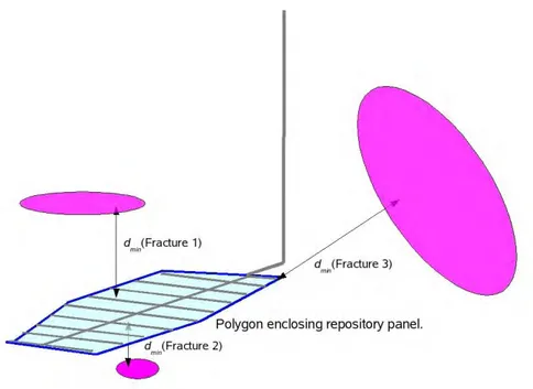
Fractures that should be represented explicitly in the model are identified as a site-specific function of fracture size, fracture transmissivity, and distance to the repository volume. The distance from a fracture to the repository vol-ume is evaluated as dmin, the minimum three-dimensional distance from any
point on the fracture to any point on a polygon in the plane of the repository, which circumscribes one of the repository panels (Figure 2.1). Successively smaller and/or less transmissive fractures are retained explicitly for smaller values of dmin.
Figure 2.1 Illustration of the minimum distance dmin from a given fracture to the polygon enclosing a repository
panel in the horizontal plane, which is used as criterion for deciding which fractures should be retained explicitly in the model, versus which fractures should be represented in terms of aggregate block-scale prop-erties.
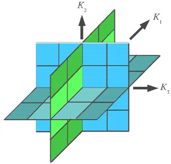
Fractures that are not represented explicitly in the model are considered to contribute to the 3-D hydraulic conductivity tensor K of the rock block that contains them. The contribution of each fracture to the block-scale tensor K is calculated by the method of Snow (1969), which is defined for infinite fractures, normalized for the finite area of the fracture in relation to block volume. Each rock block is then represented in the discrete-feature model by a set of three orthogonal features, which are divided into patches of different properties as illustrated in Figure 2.2. The transmissivities of the patches on the features that reproduce the diagonal components of the hydraulic con-ductivity tensor K11, K22, and K33 are calculated by an inverse method.
Block-scale porosity is calculated as a scalar property by adding up the con-tributions due to the transport aperture and areas of individual fractures. For mathematical details of this approach and a discussion of the simplifica-tions and their consequences, see Geier (2008a,b).
Figure 2.2 Representation of a rock block by three orthogonal features to represent block-scale hydrologic properties in the discrete-feature conceptual model.
2.1.3 Conditional representation of repository
2.1.3.1 Repository tunnels and excavation-damaged zone
The hydraulic conductivity of backfilled tunnels and the transmissive exca-vation-damaged zone (EDZ) in the wall rock along repository tunnels are represented by transmissive features configured as a tube of rectangular cross-section, along the length of each tunnel segment (Figure 2.3). Reposi-tory access tunnels (main tunnels and transport tunnels) as well as deposition tunnels are represented in this fashion. These tubes are slightly larger than the actual tunnels (by 1 m on each side), to account for the extent of the ex-cavation-disturbed zone (EDZ) into the wall rock. Transmissivity and transport aperture values are assigned to these features such that the total conductance of the tunnel cross section is reproduced.
2.1.3.2 Waste-deposition holes
Canister positions along the deposition tunnels are chosen for each realiza-tion of the discrete-fracture network, according to the full-perimeter intersec-tion criterion (FPC) as described in the SR-Can Main Report and by Munier et al. (2006). This is done with the program repository which is part of the DFM software toolkit (Geier, 2008b).
For each deposition tunnel, full-perimeter intersections (FPIs) are identified as the simulated fractures that cross all surfaces (top, bottom, and sides) of the tunnel. Deposition hole positions are then chosen sequentially by the following procedure, avoiding positions in which the canister would be in-tersected by an FPI fracture:
Starting from the entrance of the deposition tunnel, the first part of length
lplug is avoided (see Figure 2.4) in order to allow room for a sealing plug, as
specified in the D1 repository design (Brantberger et al., 2006). A trial position is tested to see if:
1. It meets respect-distance criteria for any nearby deterministic deforma-tion zones,
2. It meets the FPC criterion (i.e., no intersections with a FPI fracture) and, 3. The total transmissivity of fractures intersected by a pilot hole would be
less than the allowable transmissivity.
If the trial position is acceptable, a deposition hole is created at the position and a new trial position is chosen a distance lspacing further along the tunnel,
where lspacing is the design spacing between canisters, based on thermal
crite-ria. If the trial position is rejected, a new trial position is chosen by advanc-ing a small distance lstep along the tunnel and repeating the tests, until an
acceptable position is found.
The deposition holes for accepted position are represented by vertical, inter-nal boundaries of hexagointer-nal cross-section, starting from the floor of the tun-nel and extending to the depth specified in the design.
2.1.3.3 Calculation of utilization factor
The deposition-tunnel utilization factor is calculated as:
i i usable, spacing acceptL
l
N
=
ε
where Naccept is the number of accepted positions and Lusable,iis the "usable"
length of the ith deposition tunnel, after subtracting the portions that are reserved for the plug at the start and for clearance at the blind end of each
Figure 2.4 Illustration of method for selecting deposition-hole positions, with accepted positions in green and
rejected positions (due to full-perimeter intersection criterion) in red. The shaded area at the left side of the diagram represents the space reserved for a plug at the start of the tunnel.
2.1.4 Representation of boundary conditions
The external boundary of each model is a box with rectangular sides. Boundary conditions are imposed at intersections between discrete features and the sides of this box (lower and lateral boundary segments), as well as at the nodes (vertices) of the topographic feature at the upper surface.
Two types of external boundary condition are used:
Specified head, where the head h is specified at each node on the boundary
segment.
Specified flux, where the flux q is specified at each node (most commonly
q = 0 for no-flow boundaries).
Deposition holes are represented as passive internal boundaries with net flow equal to zero. However, flow may enter and leave the deposition holes while maintaining zero net flow.
2.1.5 Model assembly
For each realization of the stochastic DFN submodel, the discrete-feature model is assembled from a set of "panel" files that describe the geometry of the components described in the foregoing sections:
Outer boundary Topography
Deterministic deformation zones
Stochastic realization of the DFN population (retained features)
Equivalent features for block-scale representation of stochastic fractures
that are not explicitly retained.
Repository tunnel/EDZ features,
Deposition holes conditioned on the DFN realization.
To permit numerical modelling of flow and transport for a given realization of a discrete-fracture network model and conditional representation of the repository, the network comprising all of these discrete features is discre-tized to form a computational mesh, which consists of 2-D, triangular finite elements that interconnect in 3-D.
The computational mesh is produced by finding all intersections among these features, then triangulating each feature so that the geometry is defined by a series of nodes (vertices with 3-D coordinates) and triangular elements, each with transmissivity, transport aperture , and storativity corresponding to the feature from which they were derived. This is accomplished by the pro-gram meshgenx, which is part of the DFM software toolkit (Geier, 2008b).
2.2 Flow modelling
2.2.1 Groundwater flow equations
Within each planar segment of a feature, groundwater flow is governed by the 2-D transient flow equation:
T h
= q
ξ t h S where S and T are respectively the local storativity and transmissivity, h is hydraulic head, t is time, and q is a source/sink term which is zero every-where except at the specified boundaries. In the present work, S and T are assumed to be homogeneous within a given triangular segment. Conserva-tion of mass and continuity of hydraulic head are required between seg-ments, and at intersections between features.
All cases modelled in this study are for steady-state flow, in which case the time derivative is zero and the local flow equation simplifies to:
T
h
=
q
ξ
2.2.2 Finite-element approximation
The steady-state groundwater flow equation is applied to the discrete geome-try represented by the computational mesh, by use of the Galerkin finite-element method. This leads to a system of linear algebraic equations of the form:
q
=
Ah
where A is a sparse, diagonally dominant, banded matrix with coefficients depending only upon the transmissivity and geometry of each triangular element, h is a column vector of steady-state head values at the element ver-tices, and q is a column vector of unbalanced flux values at the verver-tices, equal to zero except at physical boundaries where inflow or outflow occurs. Mathematical details are given by Geier (2005).
Features that are not connected to a specified-head boundary (either directly or indirectly via connections with other features and/or net-specified-flux boundaries) are indeterminate and are not represented in the matrix equa-tions. These features constitute hydraulically isolated networks.
2.2.3 Solution of flow equations
Solutions to the systems of linear algebraic equations for the steady-state case are obtained using a standard sparse-matrix method, conjugate-gradient
method preconditioned by simple diagonal scaling, to minimize a global error measure.
Experience with solving flow equations on discrete-feature networks has shown that iterative solvers can give locally poor results for branches of a network that are isolated from the main flowing branches by tight (low-transmissivity) sections that function as “bottlenecks.” A multi-step solution approach was therefore used, in which each step consisted of the following two substeps:
Conjugate-gradient minimization of global error measure.
Local smoothing by iteratively boosting heads of internal nodes that are
surrounded by nodes with higher heads.
The local-smoothing method is implemented in Version 2.32 of the dfm module of the DFM toolkit (Geier, 2010).
2.2.4 Calculation of flows to canister positions
Flows to canister positions are calculated in the DFM module meshtrkr, as the sum of all positive flows into the deposition hole (generally balanced by outflows).
2.3 Transport modelling
2.3.1 Advective-dispersive particle-tracking
To characterize transport paths, advective-dispersive transport of nonsorbing solute in the 3-D network (for the case of no matrix diffusion) is modelled by the discrete-parcel random walk method (Ahlstrom et al., 1977). This approach represents local, 2-D advective-dispersive transport within each fracture plane. 3-D network dispersion, due to the interconnectivity among discrete features, arises as the result of local dispersion in combination with mixing across fracture intersections.
For mathematical details of the algorithm, definition of parameters and a description of its implementation in the meshtrkr module of the DFM toolkit, see Geier (2005; 2008b). The algorithm as implemented assumes complete mixing at fracture intersections; this is a reasonable approximation for the low advective flow velocities expected in a post-closure repository, as dis-cussed by Geier (2008a).
Particles are initiated at source locations. In the present study, the sources are considered to be the perimeters of the deposition holes, which are inter-nal boundaries to the mesh as described in Section 2.1.4.
2.3.2 Calculation of transport parameters
Advective-dispersive particle trajectories are traced for multiple particles for each deposition hole in the repository. For each release-path trajectory τ consisting of discrete segments {τ1, τ2, ...} the following quantities are
calcu-lated by summing over the segments τi:
i T i i τ i i w rτ
b
Δt
=
τ
v
Δl
τ
a
=
F
2
i τ r=
Δl
L
i τ r=
Δt
t
i τ T i i τ i w aτ
b
Δl
=
Δl
τ
a
=
I
2
i τ i T b=
b
τ
Δl
I
i τ i c=
T
τ
Δl
I
where ∆l and ∆t are the increments of distance and time for each step, aw=
2/bT is the local wetted surface per unit volume water, T is the local
trans-missivity, and v = ∆l/∆t is the magnitude of the local advective velocity. The same quantities are also calculated for each class of features Φ along each path:
Φb τ Δt = F i τ T i rΦ 2
Φ Δl = L i τ rΦ
Φ Δt = t i τ rΦ
Φb τ Δl = I i τ T i aΦ 2
Φ Δl τ b = I i τ i T bΦ
Φ Δl τ T = I i τ i cΦThe location, local fluid velocity, and aperture at the source are also re-corded, along with the exit location which can subsequently be related to the biosphere receptor (lake, sea, mire etc.) in the landscape for risk calculations. For detailed models of transport along streamlines, the properties of features traversed by each particle are also recorded.
In some calculation cases the excavation-disturbed zone (EDZ) around the deposition tunnels forms an important path for transport. Hence particles released from a source Si at one deposition hole may travel along the tunnel
and arrive at another deposition hole Sj before they continue along the way to
the surface. The properties of the release paths represented by such particles can be found by convolution of the distributions of properties for paths from
3. Calculations
The model used for calculations is a discrete-feature model (DFM) imple-mentation of SKB's SDM-Site site descriptive model for Forsmark, as de-fined upon completion of the surface-based investigation phase (SKB, 2008). This site descriptive model is the basis for site-specific calculations in the SR-Site safety assessment. Hence it provides the most relevant starting point for research of scientific issues that affect repository safety at these sites. Post-closure, saturated conditions are assumed unless otherwise noted. The model includes site-specific representation of the repository layout ac-cording to SKB's D1 design (Brantberger et al., 2006). While this design is adapted to an earlier version of the site descriptive model, it was the most current layout that was available at the outset of the project.
Backfill, buffer, and excavation-damage zone (EDZ) permeabilities for the base case are represented as equivalent discrete-features according to design specifications used in SKB's SR-Can safety assessment study (SKB
2006a,b). Deposition holes are placed consistent with SKB's criteria for avoiding discriminating fractures study (Munier, 2006). Post-closure, satu-rated conditions are assumed unless otherwise noted.
The base case model for each site represents late-temperate conditions, with flow simply in response to topographic gradients (though the influence of salinity is not taken into account).
3.1 Sources of data
The main source of site-specific data is the Site Descriptive Model (SDM),as described in the SDM-Site report (SKB, 2008) and supporting reports as referenced therein, most importantly the analysis of fracture data (SKB 46) and regional and site-scale hydrogeological modelling (SKB R-07-48, R-07-49, R-08-23 & R-08-95). Information on the repository design for Can is taken from the Can Main Report (SKB 2006b) and the SR-Can Data Report (SKB TR-06-25), and from the D1 design report for Fors-mark (R-06-34).
In addition, deliveries of data from SKB's SICADA and GIS databases were used as the source of coordinates for deformation zones, fracture domains, and topographic/bathymetric elevations. In general these data were trans-formed from formats used in SKB's databases to more generic formats, and provided as deliveries to the DFM modelling effort by Geosigma AB, Upp-sala.
The general approach has been to adopt SKB's descriptions directly for the base-case models, without introducing other information that has been de-veloped in the course of Field Technical Reviews or other review activities of SSM's INSITE review group. Such information may eventually inform the selection of alternative models, model variants, and scenarios for future calculations, but for the present work the focus has been on implementing a straight adaptation of SKB's SDM-Site model.
3.2 Coordinate system and domain boundary
3.2.1 Coordinate system
In contrast to the previous DFM model of Forsmark by Geier (2008a), the model presented here was developed in using the Swedish Land Survey's regional coordinate system (RAK) rather than a local coordinate system. The X coordinate is thus the Easting coordinate in the RAK system, and the Y coordinate is the Northing coordinate in the RAK system. The vertical (Z) coordinate is taken in reference to mean sea level.
3.2.2 Domain boundary
The domain boundary for the Forsmark DFM model is defined as a rectan-gular box with corners at an angle to the regional coordinate system, see Table 3.1. The lower boundary of the box is set at Z = -2100 m to conform to SKB's model. The upper boundary of the box is arbitrarily set at Z = 100 m which is high enough to avoid the topography.
Corner X (easting) Y (northing)
West 1625400 6699300
North 1636007 6709907
East 1643785 6702129
South 1633178 6691522
Table 3.1: Corners of area covered by Forsmark model domain (RAK coordinate system), based on SKB
3.3 Deterministic structures
3.3.1 Topographic feature
A DFM representation of the topographic surface were derived from SKB data delivery Elevation data 090821. The elevation and soil depth data were converted to ESRI raster format by Geosigma AB, respectively as:
rastert_eufmhoj1 fm.txt rastert_osfmgeo1 fm.txt
These data were then were converted to DFM panel format. The resulting surface feature (based on the elevation data) is shown in Figure 3.1. For the base-case variant, the transmissivity of this feature is arbitrarily set to T=10-5
m2/s, and aperture is set to b
T= 1 cm. Soil depth data have not been used in
the present stage of modelling, but could be used to assign varying hydraulic properties to the topographic feature for more detailed model variants.
Figure 3.1 Surface feature for Forsmark, discretized as right triangular panels and colored to show
topog-raphic/bathymetric elevations (red area is >10 m above sea level; dark blue is >10 m below sea level). Note that in this dataset, elevation data are missing from the NW portion of the area (west of the island of Gräsö) but this is outside the modelled region. The area of this plot covers RAK 1619990.000 E, 6714990.000 N (NW corner) to RAK 1649990.000 E, 6684990.000 N (SE corner). Triangles are 100 m high by 100 m wide.
3.3.2 Deformation zones
3.2.2.1 Geometry of deformation zones
The geometry of deformation zones is taken from files provided as a data delivery by SKB, and then converted to AutoCAD DXF format by Geo-sigma AB, as two files:
DZ_PFM_Loc_v22_01 basemod_joel.dxf DZ_PFM_REG_v22.02 basemod_joel.dxf
for the local and regional model scales, respectively. For use in the DFM model, these were then converted to the panel file format as:
DZ_FM_loc_v22_basemod.pan DZ_FM_reg_v22_basemod.pan
The geometry of the deformation zones on the two scales is shown in Fig-ures 3.2 and 3.3.
The deformation zones are defined as surfaces enclosing approximately tabular volumes, rather than as simple tabular surfaces. This is in contrast to the representation that was used in previous DFM models. In this DFM ad-aptation, the bounding surface of each deformation zone is treated as a dis-crete feature. Since there are normally two sides to each deformation zone at a given point, the hydraulic properties are distributed equally between the two sides (in other words, each surface belonging to either side of the de-formation zone is assigned half of the transmissivity and half of the transport aperture for a given point).
Figure 3.2 Plan view of deformation zones in the local model area, discretized as triangles. Color scale
indicates elevations, ranging from dark blue at the base of the modelling volume (Z = -2100 m) to red at the surface.
Figure 3.3 Plan view of deformation zones in the regional model area, discretized as triangles. Color scale
indicates elevations, ranging from dark blue at the base of the modelling volume (Z = -2100 m) to red at the surface.
3.3.2.2 Hydraulic properties of deformation zones
Hydraulic properties for the deformation zones in the base-case model were assigned based on SKB's Hydraulic Conductor Domain (HCD) model as described on p. 85 of SKB R-08-95 (Follin, 2008):
z k+N
σ T
T = z y, x, T 010 / 0, log where: k = 232.5 m σlog T = 0.632and where
T
0is the geometric mean of the values of T0 calculated as:
z k T = T zi i F i F0 / 10 giving:
= n T
z n T z k = T n = i i F k z n = i i z i F
1 / 1 0 10 / 10where
z
is the mean z coordinate for the measurements in the zone.The effective transport aperture bT and storativity S are assumed to be
corre-lated to transmissivity as:
0.5 0.5 T = bT 0.5 4 10 7 T = S
consistent with Equations 8-9 and 8-11 in SKB R-05-18.
For each borehole intercept xi with a deformation zone, values of
transmis-sivity TF(xi) were taken from Table C1 of R-08-23 and assigned coordinates
in the reference system based on borehole and deformation zone geometry. Values of T0 are then calculated from these results.
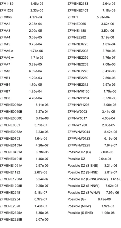
For 60 of the deformation zones that are included as HCDs in the regional or local model (Table 3.2), no transmissivity data are available from intersec-tions with boreholes from the site characterization programme. These HCDs are assigned generic values of T0 = 1x10⁻⁶ m2/s.
Two other deformation zones are intersected by boreholes but transmissivity values were not included in Table C1 of R-08-23. These are resolved as fol-lows:
ZFMENE1061B (intersects with Borehole KFM08C as DZ4 in the interval
829 – 832 m according to R-07-45, p. A15-110): Use value for ZFMENE1061A.
ZFMNNW0404 (intersects Borehole KFM01B as DZ3 in the interval 415 -
454 m and borehole KFM07A as DZ1 in the interval 180 – 185 m accord-ing to R-07-45, p. A15-55): Use generic value.
Table 3.2 List of deformation zones without transmissivity data ZFM871 ZFMA1 ZFMB23 ZFMB5 ZFMB6 ZFME1 ZFMENE0062B ZFMENE0062C ZFMENE0159B ZFMENE0169 ZFMENE0810 ZFMENE2332 ZFMEW0137 ZFMEW1156 ZFMJ1 ZFMJ2 ZFMK1 ZFMNE0808A ZFMNE0808B ZFMNE0808C ZFMNNE0828 ZFMNNE0842 ZFMNNE0860 ZFMNNE0869 ZFMNNE0929 ZFMNNE1132 ZFMNNE1133 ZFMNNE1134 ZFMNNE1135 ZFMNNE2293 ZFMNNE2308 ZFMNNW0101 ZFMNNW0823 ZFMNW0002 ZFMNW0029 ZFMNW0805 ZFMNW0806 ZFMNW0854 ZFMNW1173 ZFMWNW0001 ZFMWNW0004 ZFMWNW0016 ZFMWNW0019 ZFMWNW0023 ZFMWNW0024 ZFMWNW0035 ZFMWNW0036 ZFMWNW0809A ZFMWNW0809B ZFMWNW0813 ZFMWNW0835A ZFMWNW0835B ZFMWNW0836 ZFMWNW0851 ZFMWNW0853 ZFMWNW0974 ZFMWNW1053 ZFMWNW1056 ZFMWNW1068 ZFMWNW1127
Table 3.3 T0 values for deformation zones (in data file FMSDMSite_HCD_T0.prn) ZFM1189 1.45e-05 ZFM1203 2.33e-05 ZFM866 4.17e-04 ZFMA2 2.03e-04 ZFMA3 2.00e-05 ZFMA4 3.68e-05 ZFMA5 3.75e-04 ZFMA6-e 1.71e-06 ZFMA6-w 1.71e-06 ZFMA7 3.89e-05 ZFMA8 6.09e-04 ZFMB1 1.29e-03 ZFMB4 1.70e-05 ZFMB7 1.25e-04 ZFMB8 4.78e-04 ZFMENE0060A 5.11e-06 ZFMENE0060B 3.27e-04 ZFMENE0060C 3.49e-08 ZFMENE0061 3.73e-07 ZFMENE0062A 3.23e-06 ZFMENE0103 1.64e-06 ZFMENE0159A 4.26e-07 ZFMENE0401A 6.78e-05 ZFMENE0401B 1.46e-07 ZFMENE1061A 2.97e-06 ZFMENE1192 2.67e-08 ZFMENE1208A 5.24e-07 ZFMENE1208B 9.25e-07 ZFMENE2248 5.18e-07 ZFMENE2254 6.37e-07 ZFMENE2320 1.43e-07 ZFMENE2325A 6.35e-08 ZFMENE2325B 2.07e-05 ZFMENE2383 2.64e-06 ZFMENE2403 7.18e-09 ZFMF1 5.91e-04 ZFMNE0065 3.62e-06 ZFMNE1188 3.50e-06 ZFMNE2282 3.19e-08 ZFMNNE0725 1.81e-04 ZFMNNE2008 3.79e-06 ZFMNNE2255 1.76e-07 ZFMNNE2263 7.08e-06 ZFMNNE2273 8.41e-08 ZFMNNE2280 2.89e-06 ZFMNNE2312 9.57e-06 ZFMNNW0100 1.79e-06 ZFMNNW1204 3.59e-06 ZFMNNW1205 3.00e-08 ZFMNW0003 3.41e-05 ZFMNW0017 4.06e-04 ZFMNW1200 2.08e-05 ZFMWNW0044 8.42e-05 ZFMWNW0123 6.19e-06 ZFMWNW2225 7.64e-07 Possible DZ (G) 2.03e-06 Possible DZ 2.64e-04 Possible DZ (S-ENE) 3.21e-06 Possible DZ (S-NNE) 2.81e-07 Possible DZ (S-NNE/WNW) 1.61e-05 Possible DZ (S-NNW) 7.02e-08 Possible DZ (S-WNW) 7.95e-06 Possible (G) 8.49e-09 Possible (NNW) 1.92e-07 Possible (S-ENE) 1.06e-08
3.3.2 Shallow bedrock aquifer
Following the description on p. 45-47 of SKB R-08-23, three horizontal features are included to represent what SKB has termed the “shallow bed-rock aquifer.” These are placed at z = -25 m, z = -75 m, and z = -125 m re-spectively. Elements belonging to these features are assigned transmissivity values equal to the closest borehole measurement point for the correspond-ing depth intervals in Table 3-11 of SKB R-08-23.
A difference between this implementation and SKB's is that the shallow bedrock aquifer features are at constant depth rather than parallel to the to-pography. Also these features are rectangular in plan view, with corners as listed in Table 3.4. The coordinates limit these features to an area in which they cannot outcrop.
Corner X (easting) Y (northing)
Southwest 1630000 6699000
Southeast 1633500 6699000
Northeast 1633500 6701500
Northwest 1630000 6701500
Table 3.4: Corners of area covered by Forsmark shallow bedrock aquifer (RAK coordinate system). These
3.4 Stochastic features
3.4.1 Fracture domains
The fracture domains as defined for SDM-Site Forsmark (SKB, 2008) were obtained as part of a data delivery from SKB's SICADA database and trans-formed to AutoCAD DXF format by Geosigma AB. The special-purpose script parsedomains was used to convert these to DFM panel format, result-ing in the data file:
FD_FM_reg_v22_basemod.pan .
Next these were translated into polyhedral domains for generating fractures with the DFM module fracgen, resulting in the file:
FM_reg_v22_basemod.domains
which contains all of the fracture domains defined by SKB. Input files for each specific domains were produced by hand-editing copies of this file to delete all other domains. Finally, subdomains for different depths as speci-fied in Table C-1 of SKB R-08-95 (Follin, 2008) were defined by running the script create_depth_domains which inserts the appropriate fracgen clip-ping commands, as detailed in Table 3.5.
Fracture Domains Depth Subdomain fracgen clipping commands
shallow clipped below -200
middle clipped above -200 clipped below -400
FFM01 and FFM06
deep clipped above -400
FFM02 shallow (none needed as FFM02 only exists above –200 m)
shallow clipped below -400
FFM03, FFM04 and FFM05
deep clipped above -400
Table 3.5 Definition of fracture subdomains by depth. Note that the depth ranges for subdomains in FFM06
are the same as for FFM01, and the depth ranges for subdomains in FFM04 and FFM05 are the same as for FFM03.
3.4.2 Fracture set definitions
The fracture population for the Forsmark model is simulated based on the statistical hydro-DFN model as specified in SKB R 08-98 Table C-1 (Follin, 2008). The fracture set statistics listed in that table were transcribed directly into fracture set definitions files for fracgen input, as listed in Table 3.6.
Fracture Domains Depth Subdomain Fracture set definitions file
shallow FFM01shallow.sets middle FFM01middle.sets FFM01 and FFM06 deep FFM01deep.sets FFM02 shallow FFM02shallow.sets shallow FFM03shallow.sets FFM03, FFM04 and FFM05 deep FFM03deep.sets
Table 3.6 List of fracture set definitions files used as input to fracgen, for generating fractures in the different
fracture domains and subdomains.
3.4.3 Block-scale feature grid
Fractures are either retained explicitly or assigned to the block-scale fea-tures, depending on their proximity to polygons bounding these sets of re-pository panels in combination with their size and transmissivity. The rules for retaining fractures explicitly are specified in Table 3.7.
The grid of block-scale features covers the domain bounded by:
East side at X = 1 638 000 (RAK E) West side at X = 1 627 000 (RAK E) South side at Y = 6 697 000 (RAK N) North side at Y = 6 703 000 (RAK N) Upper boundary at Z = 0 m.a.s.l. Lower boundary at Z = -1 950 m.a.s.l.
Shell: Distance range Retain if rf is greater than: and Tf is greater than:
1 500 m < dmin ≤ 50000 m 10000 m 1×10¹⁰ m2/s
2 100 m < dmin ≤ 500 m 250 m 1×10⁻⁵ m2/s
3 50 m < dmin ≤ 100 m 100 m 1×10⁻⁵ m2/s
Table 3.7 Rules for explicitly retaining fractures of a given radius rf and transmissivity Tf when dmin is the
minimum distance from any point on the fracture to the polygon enclosing the portions of the repository being modelled (see Figure 2.1), for the Forsmark model. Note that no fractures are retained in the distance range
Figure 3.4 Plan views of the retained fractures in the stochastic DFN portion of the model around the
reposi-tory, for two realizations n = 1 and n = 2. Hexagonal fractures are shown as outlines. Fracture transmissivity is
indicated by the color scale, ranging from dark blue (Tf < 10-8) to red (Tf > 10-3). Both plots show the
Figure 3.5 Plan view of the block-scale equivalent features representing fractures removed from the
stochas-tic DFN portion of the model around the repository, for one realization (n = 1). Fracture transmissivity is
indicated by the color scale, ranging from dark blue (Tf < 3x10⁻⁴) to red (Tf > 10-2). The rectangular area of the
plot extends from RAK 1 627 000 E, 6 697 000 N to RAK 1 638 000 E, 6 703 000 N. For blocks that contain no transmissive fractures from the DFN realization, the block-scale equivalent features are omitted.
3.5 Repository layout
The layout for the Forsmark repository is based on the layout at the z = -410 m level as defined by the D1 design report (Brantberger et al., 2006). The access tunnels and deposition tunnels included in the model are shown in Figures 3.6 and 3.7.
The entire repository layout, including access tunnels, deposition tunnels, and deposition holes, is here modelled in a single run. This differs from the earlier DFM model (Geier, 2008a), in which the repository was modelled in separate runs for each of three different sections.
The parameters used to define the repository features are listed in Table 3.8.
Figure 3.6 Situation of the D1 repository layout at the Forsmark site (adapted from SKB R-06-34 Figure 5-2
by adding the diagonal grid lines which run North-South and East-West). Note this view is rotated from the reference coordinates (North is approximately 45 degrees to the left from upward in this diagram).
Parameter value Justification
Deposition hole sides 6 Hexagonal approximation to circle
Deposition hole radius 0.88 m SR-Can Initial State Report (SKB TR-06-21), Figure 5-3
Deposition hole depth 7.83 m SR-Can Initial State Report (SKB TR-06-21), Figure 5-3
Canister radius 0.53 m SR-Can Initial State Report (SKB TR-06-21), Figure 5-3
Canister length 4.83 m SR-Can Initial State Report (SKB TR-06-21), Figure 5-3
Canister top 2.5 m SR-Can Initial State Report (SKB TR-06-21), Figure 5-3
Distance between holes Lspacing 7.8 m Based on D1 repository design (Brantberger et
al., 2006)
Distance from drift end 20 m Deep Repository, Underground Design Prem-ises D1/1 (SKB R-04-60)
Distance from drift start Lplug 8 m Deep Repository, Underground Design
Prem-ises D1/1 (SKB R-04-60)
Minimum step distance Lstep 1 m Assumed generic value
Pilot hole transmissivity 1×10⁻⁵ m2/s Assumed generic value Table 3.8 Deposition hole parameters for the model.
Figure 3.7 Access & deposition tunnels (red) and deposition holes (very small blue dots) for the repository.
The deposition-hole positions vary depending on the realization of the fracture network model, with applica-tion of the deposiapplica-tion-hole criteria. Those shown in the figures are for realizaapplica-tion n = 1 of the DFN component model.
3.6 Nested model construction
The DFM model geometry for Forsmark is fully defined by the panel files that describe the components, as described in the foregoing sections. These components are first assembled in a single file which contains all of the geometric features in the model, then converted to a 3-D mesh with triangu-lar elements, for use in finite-element calculations.
For a given DFN realization n = 1, 2, etc., the panel file FMSDMfullTnc.pan is assembled from components in the following order:
Regional model boundary (FM23RegionalBoundary3.pan) Regional deformation zones(DZ_FM_reg_v22_genericT.pan)
Local deformation zones (DZ_FM_loc_v22_genericT.pan) filtered to
re-move redundant regional deformation zones
Shallow bedrock aquifer (FM23BedrockAquifer4.pan),
Topographic feature (FM_elevation.pan) using generic values of T = 10-5
m2/s and b
T = 1 cm
Repository layout conditional on the DFN realization
(SDMFMfullTn.repos_pan)
Equivalent conductivity grid for the DFN realization
(SDMFMfullTn.kgrid_pan)
Discrete fractures retained from the DFN realization
(SDMFMfullTn.fracs_pan)
The deformation zone data supplied by SKB included regional deformation zones in the file for local deformation zones, so the redundant versions of the regional zones were filtered out during assembly of the panel file. Figure 3.8 shows the assembled features in plan view.
Figure 3.9 shows a cross section through a section of the repository at -410 m. Note that some local deformation zones (seen as pairs of parallel lines in yellow) as well as orthogonal grid features (in red) pass through deposition tunnels. The D1 repository layout used here does not account for the positions of some major zones that have shifted in the SDM-Site struc-tural geological model. These features were not included the repository runs, so the resulting layout may contain a few deposition holes that are inter-sected directly by deformation zones.
The assembled features are then converted into a triangular finite-element mesh file using the DFM module meshgenx (with postprocessing script
tri-postx). Figure 3.10 shows a horizontal section through the repository area of
the resulting mesh. The identities of the original features are retained for each triangular element in the mesh, so that the hydrologic properties of individual features can be modified depending on the realization.
Figure 3.8 Combined plot of all panels for Realization 1. Black rectangle shows external boundary of DFM
Figure 3.9 Horizontal section through repository area of combined panels at Z = -410 m. The color scale
indicates transmissivity of the discrete features that intersect the plane of the section; dark blue indicates T <
10-8 m2/s while red indicates T > 10-4 m2/s. The access and deposition tunnels of the repository appear as
green lines and deposition holes appear as blue dots. Note that final transmissivities of some features are assigned at a later stage, following mesh generation.
Figure 3.10 Horizontal section through repository area of mesh at Z = -410 m. The color scale indicates
transmissivity of the discrete features that intersect the plane of the section; dark blue indicates T < 10-10 m2/s
3.7 Flow calculations
3.7.1 Boundary conditions
The boundary conditions (Table 3.9) were chosen to approximate a situation similar to the present day at Forsmark.
For portions of the topographic upper surface that are at or above sea level, the head is set equal to equal to the elevation Z.
For portions of the topographic surface that are below sea level, a fixed head is assigned equal to zero (the present-day mean sea level, used as a datum). Note that this approach will somewhat exaggerate the pressure gradients (modelled as equivalent freshwater head gradients) through the model, since in reality the groundwater pressures at the seabed will be higher due to the salinity of the water column.
Linearly varying heads to approximate the topographic gradient are applied along each of the lateral boundaries (based on a linear fit to the topography along that edge of the model), with a restriction that the head must be at least equal to sea level.
A no-flow condition is implicitly specified at the base. This is consistent with a hypothesis that the bedrock becomes extremely low in permeability at depth.
Boundary Boundary Condition Type
Value
Seafloor Specified head h = 0
Land surface Specified head h = max( 0, Z )
Bottom Specified flux q = 0
Southwest side Specified head h = max( 0, -0.000505 X + 0.000505 Y – 2549.53 m )
Southeast side Specified head h = max( 0, 0.000806 X + 0.000806 Y – 6713.51 m )
Northeast side Specified head h = max( 0, 0.000041 X – 0.000041 Y + 217.95 m )
Northwest side Specified head h = max( 0, -0.000445 X – 0.000445 Y + 3716.48 m )
3.7.2 Flow solution
A solution for steady-state flow through the discrete-feature network was obtained using a modified conjugate-gradient method with diagonal precon-ditioning and 10 local-smoothing steps, allowing for 80,000 iterations of the conjugate-gradient solver per step. The resulting head field in the plane of the repository is shown in Figure 3.11.
Figure 3.11 Horizontal section through repository area of mesh at Z = -410 m. The color scale indicates the
calculated heads along the discrete features that intersect the plane of the section; dark blue indicates h < 0.2 m while red indicates h > 1 m. This is the same cross-sectional area and realization as shown in Figure 3.10.
3.8 Particle tracking
Advective-dispersive particle tracking is performed using the meshtrkr mod-ule using the mesh file for a given realization, plus the calculated head vec-tor. For each canister position that is intersected by a transmissive feature, 100 particles are released. Transport parameters used in this step are summa-rized in Table 3.10.
Table 3.10 Parameters for advective-dispersive particle tracking.
Parameter Feature Category Feature Set(s) Value
Molecular diffusion coefficient All 1 to 68 2.0x10 -9 m2/s Ratio of transverse dispersivity to longitudi-nal dispersivity All 1 to 68 0.1
Major deformation zones 1 10 m
Shallow bedrock aquifer 2 10 m
Quaternary deposits 3 5 m
Repository tunnels 4 1 m
Longitudinal dispersivity
4. Results and discussion
4.1 Practical aspects
Although not the primary objective of this modelling project, experiences regarding the practicality of applying the DFM approach to SKB's site de-scriptive model is expected to be useful for planning use of this approach to support review of an upcoming license application, base on these same data. With an eye toward the quality assurance demands of such applications, an effort was made to make the links from the site descriptive model to the computational model as direct as possible. This approach, combined with the increased complexity of the SDM-Site model relative to previous versions of SKB's site descriptive model for Forsmark, resulted in several unanticipated problems that required a large effort.
The number of panels that go into a typical realization of the Forsmark model are listed by component in Table 4.1. This leads to a mesh with ap-proximately 2.5 million nodes, 5.8 million elements, and representing 112,000 features. It may be noticed from table 4.1 that the number of sto-chastic fractures retained from the DFN component are a fairly small part of the overall model, while the equivalent conductivity grid, repository tunnels, and deformation zones make up a dominant portion. This suggests that a somewhat more detailed representation of the rather sparse fracture popula-tion in the near field should be possible, even while reducing the overall size of the model (in terms of numerical complexity) by a reduction in the resolu-tion of the equivalent conductivity grid features.
The usefulness of the DFM model is limited by the time needed to construct a mesh for a given realization of the stochastic DFN, and calculate flow and transport. Table 4.2 lists the computational time required for key stages of the modelling process for the Forsmark model presented here. Following improvements to the mesh generation portion of the package, the slowest stage of the process is the flow simulation (dfm module).
The dominant part of the process, in terms of computational time involves set-up and iterative solution of the flow matrices. The time needed for this stage scales roughly as N3, where N is the number of nodes in the finite
ele-ment mesh. Thus a 50% reduction in the number of nodes in the problem could reduce simulation time by close to a factor of 10.
Memory requirements can also be significant, particularly the peak storage that is needed while forming element matrices. Using compact matrix stor-age, a problem with 2.5 million nodes required peak storage of 960 Mb while forming matrices, and 41 Mb for the final compact matrix.
Feature category Approximate number of panels in a single realization
Regional deformation zones 76,000
Local deformation zones (including shallow bedrock aquifer) 69,000
Topographic features (part within regional model area) 16,500
DFN fractures retained in near-field 1,500
Equivalent conductivity grid features 216,000
Repository tunnels and deposition holes 67,000
Table 4.1 Number of panels comprising major components of the DFM model for Forsmark.
Stage Typical time (hrs)
Stochastic DFN generation (per realization) 5
Repository (conditional layout) <0.05
Panel assembly < 0.25
Mesh generation (calculate intersections among panels) 44
Mesh generation (triangulate all panels) 18
Mesh generation (consolidate triangulation) <0.5
Flow simulation (build reduced flow matrices) 48
Flow simulation (per local smoothing step with 80,000 iterations) 22
Particle tracking (for 100 particles per deposition hole location) 5
Table 4.2 Time requirements for key stages of DFM model construction, flow and transport simulation for the
mode based on SDM-Site Forsmark. Run times are for an IBM M55 tower configured with dual Intel Core 2 processors (2.13 GHz CPU clock speed) and 2.9 GiB memory (667 MHz). Note that each process typically only uses one of the dual processors at a time.
4.2 Utilization of deposition tunnels
The utilization factor ε for Forsmark is found to be better than 80% for two realizations (Table 4.3), after accounting for deposition-hole positions that are rejected either because they violate the full-perimeter intersection crite-rion (FPC) or because the pilot-hole transmissivity exceeds 10-5 m2/s. As in
previous models (Geier, 2008a), the difference in ε between realizations is only a few percent.
The utilization is 10-15% higher than results obtained from the previous version of the DFM model of Forsmark (Geier, 2008a), and thus closer to estimates obtained by SKB for the SR-Can safety assessment exercise (SKB, 2006a). The difference is believed to be due to more uniform simulation of fracture centres in the fracture domains (and thus reduced finite-domain ef-fects), using the new algorithm mentioned in Section 4.1.1.
Realization Total tunnel length (m) Usable length (m) Trial positions accepted Utilization Positions Rejected (FPC) Positions Rejected (pilot hole) 1 48469.8 43233.8 4567 82.4% 7894 8 2 48469.8 43233.8 4699 84.8% 6822 63
Table 4.3 Utilization of deposition tunnels for Forsmark base case DFN model (two realizations). Note that the
number of trial positions accepted is based on a minimum centre-to-centre distance between canisters of 7.8 m; more canisters could be accommodated by using a smaller spacing adapted to the rock type and local thermal properties, as has been done in SKB's design work (Brantberger et al., 2006).
4.3 Flow rates to deposition holes
The cumulative distribution of flow rates to deposition holes from the first realization of the DFM model is shown in Figure 4.1. This can be compared with solution, which can be compared with Figure 4.2 on p. 47 of SKI 2008:11 (Geier, 2008a). The mid-temperate variant of the previous model is the most nearly comparable to this mode, in terms of boundary conditions and assumptions.
The most noticeable difference with the earlier models is that 52% of the deposition holes show no measurable flow, despite that they are intersected by transmissive features (fractures, deformation zones, or EDZ features be-low the tunnel floor). For deposition holes that are intersected by fbe-lowing features, the median flow rate is increased by approximately an order of magnitude relative to the earlier model.
A few of the highest flow rates may be for deposition holes that are inter-sected by deformation zones or orthogonal grid features, as these have not been screened out of this simulation. As noted previously, the D1 repository layout (Brantberger et al., 2006) is not adapted to the final positions of de-formation zones in the SDM-Site model. This should be corrected in future applications of this model by using the updated D2 layout. However, these results may be viewed as illustrative (pessimistically) of the potential conse-quences of inaccurate identification of deformation zones and their positions in a repository.
4.4 Discharge paths
Initial results from the particle-tracking runs showed a very high percentage of particles getting stuck, due to locally poor precision in the head solution. 14,197 of the particles (representing 6%of particles released at all holes with numerically significant flows) ended up at other deposition holes. This is consistent with the result from the previous DFM model of the Forsmark site (Geier, 2008b) showing that, in the sparsely fractured rock at Forsmark, transport is strongly along the EDZ.
The 115 particles that arrive to shallow depths (<50 m) based on a partial solution of the flow problem (Figure 4.2) were highly concentrated at a few locations in the mesh. Most were so tightly clustered that they plot essen-tially on top of each other in this figure. This is believed to be a modelling artefact due to too coarse of resolution in the far-field DFM model, rather than a result to be trusted. Results might be improved by:
Improved discretization of local-scale deformation zones that are likely to
serve as transport paths to the surface;
Simplifications of other parts of the model that are found to be of little
importance for results at this level of detail, in order to reduce the com-plexity of the flow problem;
Further iterative refinement of the flow solution.
Due to the extremely limited number of particle arrivals to the surface, a quantitative summary of results is not presented. However Table 4.4 give an example of the type of results obtained for a single particle that originates in the EDZ connecting to a deposition hole, and finds its way to the surface via three different sets of discrete fractures in the near-field, deformation zones, shallow bedrock aquifer and finally Quaternary deposits. In this example, retention takes place predominantly in the deformation zone and secondarily in the tunnels and EDZ.
Figure 4.2 Areal distribution of arrivals to the near-surface environment for Forsmark DFM model, Realization
1, particle tracking based on Step 7 of flow solution.
Integrals: ∆L(m) ∆t (s) T∆L(m3/s) b∆L(m2) aw∆L (-) ∆F (s/m)
All Sets 3.1E+03 8.8E+07 7.1E-01 7.0E-03 4.6E+09 5.8E+14
Set 1 1.2E+03 8.7E+07 5.3E-01 3.4E-03 3.2E+09 5.8E+14
Set 2 2.5E+01 2.0E+05 2.0E-04 1.7E-05 6.9E+07 6.1E+11
Set 4 1.9E+03 1.6E+06 1.8E-01 3.7E-03 1.1E+09 1.1E+12
Set 13 4.9E-03 1.4E+00 6.5E-10 5.8E-10 4.2E+04 1.2E+07
Set 18 1.0E+01 5.6E+04 2.8E-07 7.1E-07 1.5E+08 8.1E+11
Set 45 1.1E-02 5.9E-01 1.5E-08 2.8E-09 4.3E+04 2.3E+06
Table 4.4 Example of summary statistics for a particle originating at deposition hole 922 at X = 1630731.7 m,
Y = 6700126.2 m, Z = 411.0 m (entering the EDZ) and ending at X = 1631514.8 m, Y = 6701275.2 m, Z =
5. Conclusions
5.1 Practicality of modelling approach
The implementation of the SDM-Site model for Forsmark was hindered by several major practical difficulties, resulting in part from increased complex-ity of the site descriptive model, and in part software bugs including a loss-of-precision error due to a shift to regional rather than local coordinates. After fixing these problems, the DFM model appears to be practical with a modelling cycle of about two weeks per realization. Most of this time is for the flow solution, which scales approximately as the cube of the number of nodes in the finite element mesh.
Therefore the best prospects for reductions in simulation time and/or attain-ment of higher numerical precision in the results appear to be via decreasing the number of nodes in the model. This can most easily accomplished by a lower resolution in the equivalent-conductivity feature grid, which might allow increased resolution of the stochastic DFN in the near field of the re-pository.
5.2 Utilization factors
An improvement in utilization factors of 10% to 15% relative to the previous Forsmark DFM model was obtained. This is closer to SKB's results in SR-Can (SKB, 2006), and is believed to be a result of an improved DFN genera-tion algorithm that produces more a more spatially uniform distribugenera-tion of fracture centres in polyhedral domains.
Variability between DFN realizations was found to be small (less than a 3% difference between the two realizations that were produced for the Forsmark base-case DFN model) in the previous model.
5.3 Flow through deposition holes
Slightly more than half of all deposition holes are found to be non-flowing even though intersected by EDZ features and in some cases isolated frac-tures. This is believed to be a consequence of a poorly connected fracture system with relatively few conductive paths, resulting in many stagnant zones even among the hydraulically connected features.
Among deposition holes that are intersected by flowing features, the median flow rate is about a factor of 10 higher than was estimated from DFM
mod-due to deformation zones that (according to the SDM-Site model) are in different positions than was planned for in the D1 repository layout.
5.4 Transport paths
Results of particle tracking support the result from the previous DFM model for Forsmark, that the excavation-disturbed zone around deposition tunnels and access tunnels in the repository are an important transport path, with solute often finding its way along tunnels to other deposition holes.
Due to a high percentage of particles that become stuck due to local impreci-sion in the flow solution, further analysis of results is not deemed to be justi-fied. Improved precision in the flow field, and hence more reliable particle-tracking results, might be obtained by judicious simplifications in the model to speed numerical convergence of the flow solution.