Report number: 2008:01 ISSN: 2000-0456 Available at www.stralsakerhetsmyndigheten.se
A combined deterministic and
probabilistic procedure for safety
assessment of components with
cracks – Handbook
Research
2008:01
Authors: Peter DillströmMats Bergman Björn Brickstad Weilin Zang Iradj Sattari-Far Peder Andersson Göran Sund Lars Dahlberg Fred Nilsson
Title: A combined deterministic and probabilistic procedure for safety assessment of compo-nents with cracks – Handbook.
Report number: 2008:01
Author/Authors: Peter Dillström, Mats Bergman, Björn Brickstad, Weilin Zang, Iradj Sattari-Far, Peder Andersson, Göran Sund, Lars Dahlberg and Fred Nilsson
Name of your company or institution/city and country: DNV Technology Sweden (now Inspecta Technology AB)/Stockholm Sweden.
This report concerns a study which has been conducted for the Swedish Radia-tion Safety Authority, SSM. The conclusions and viewpoints presented in the report are those of the author/authors and do not necessarily coincide with those of the SSM.
Background
SSM has supported research work for the further development of a previously developed procedure/handbook (SKI Report 99:49) for as-sessment of detected cracks and tolerance for defect analysis. During the operative use of the handbook it was identified needs to update the deterministic part of the procedure and to introduce a new probabilistic flaw evaluation procedure. Another identified need was a better descrip-tion of the theoretical basis to the computer program.
The project was initiated by SKI.
Objectives of the project
The principal aim of the project has been to update the deterministic part of the recently developed procedure and to introduce a new proba-bilistic flaw evaluation procedure. Other objectives of the project have been to validate the conservatism of the procedure, make the procedure well defined and easy to use and make the handbook that documents the procedure as complete as possible.
Results
The procedure/handbook and computer program ProSACC, Probabilis-tic Safety Assessment of Components with Cracks, has been extensively revised within this project.
The major differences compared to the last revision are within the fol-lowing areas:
• It is now possible to deal with a combination of deterministic and probabilistic data.
• It is possible to include J-controlled stable crack growth.
• The appendices on material data to be used for nuclear applica-tions and on residual stresses are revised.
• A new deterministic safety evaluation system is included.
• The conservatism in the method for evaluation of the secondary stresses for ductile materials is reduced.
• A new geometry, a circular bar with a circumferential surface crack has been introduced.
Effect on SSM supervisory and regulatory task
The results of this project will be of use to SSM in safety assessments of components with cracks and in assessments of the interval between the inspections of components in nuclear power plants.
Project information
SSM´s Project Leader: Kostas Xanthopoulos Project number: 14.42-000696/00202.
Project Organisation: DNV Technology Sweden (now Inspecta Techno-logy AB) has managed the project with P. Dillström as project leader. M. Bergman, B. Brickstad, W. Zang, I. Sattari-Far, P. Andersson, G. Sund, L. Dahlberg and F. Nilsson have assisted in the development of the project.
Table of Content
Page
NOMENCLATURE...8 1. INTRODUCTION... 13 1.1 References ... 15 2. PROCEDURE ... 16 2.1 Overview ... 16 2.2 Characterization of defect... 17 2.3 Choice of geometry... 17 2.4 Stress state ... 17 2.5 Material data ... 182.6 Calculation of slow crack growth ... 19
2.7 Calculation of K and Ip I s K ... 20 2.8 Calculation of L ... 21 r 2.9 Calculation of K ... 21 r 2.10 Fracture assessment... 22 2.11 Safety assessment... 24 2.12 References ... 27 TABLE OF REVISIONS ... 28
APPENDIX A. DEFECT CHARACTERIZATION... 29
A1. Defect geometry... 29
A2. Interaction between neighbouring defects... 30
A3. References ... 32
APPENDIX R. RESIDUAL STRESSES ... 33
R1. Butt welded joints ... 34
R1.1 Thin plates ... 34
R1.2 Thick plates ... 35
R1.3 Butt welded pipes... 36
R1.4 Butt-welded bimetallic pipes (V or U shape) ... 38
R1.5 Butt-welded bimetallic pipes (X shape) ... 43
R1.6 Pipe seam welds... 45
R2. Fillet welds ... 45
R3. Stress relieved joints ... 45
R4. Summary... 46
R5. References ... 47
APPENDIX G. GEOMETRIES TREATED IN THIS HANDBOOK... 48
G1. Cracks in a plate... 48
G1.1 Finite surface crack ... 48
G1.2 Infinite surface crack... 49
G1.3 Embedded crack... 50
G1.4 Through-thickness crack ... 51
G2. Axial cracks in a cylinder ... 52
G2.1 Finite internal surface crack ... 52
G2.2 Infinite internal surface crack ... 53
G2.3 Finite external surface crack... 54
G2.4 Infinite external surface crack ... 55
G2.5 Through-thickness crack ... 56
G3. Circumferential cracks in a cylinder ... 57
G3.1 Part circumferential internal surface crack... 57
G3.2 Complete circumferential internal surface crack ... 58
G3.3 Part circumferential external surface crack ... 59
G3.4 Complete circumferential external surface crack ... 60
G3.5 Through-thickness crack ... 61
G4. Cracks in a sphere ... 62
G4.1 Through-thickness crack ... 62
G5. Cracks in a bar ... 63
G5.1 Part circumferential surface crack ... 63
APPENDIX K. STRESS INTENSITY FACTOR SOLUTIONS... 64
K1. Cracks in a plate... 64
K1.1 Finite surface crack ... 64
K1.2 Infinite surface crack... 69
K1.3 Embedded crack... 71
K1.4 Through-thickness crack ... 74
K2. Axial cracks in a cylinder ... 75
K2.1 Finite internal surface crack ... 75
K2.2 Infinite internal surface crack ... 78
K2.3 Finite external surface crack... 80
K2.4 Infinite external surface crack ... 83
K2.5 Through-thickness crack ... 85
K3. Circumferential cracks in a cylinder ... 92
K3.1 Part circumferential internal surface crack... 92
K3.2 Complete circumferential internal surface crack ... 105
K3.3 Part circumferential external surface crack ... 107
K3.4 Complete circumferential external surface crack ... 110
K3.5 Through-thickness crack ... 112
K4. Cracks in a sphere ... 119
K4.1 Through-thickness crack ... 119
K5. Cracks in a bar ... 121
K5.1 Part circumferential surface crack ... 121
K5. References ... 124
APPENDIX L. LIMIT LOAD SOLUTIONS... 125
L1. Cracks in a plate... 125
L1.1 Finite surface crack ... 125
L1.2 Infinite surface crack... 126
L1.3 Embedded crack... 127
L1.4 Through-thickness crack ... 128
L2. Axial cracks in a cylinder ... 129
L2.1 Finite internal surface crack ... 129
L2.2 Infinite internal surface crack ... 130
L2.3 Finite external surface crack... 131
L2.4 Infinite external surface crack ... 132
L2.5 Through-thickness crack ... 133
L3. Circumferential cracks in a cylinder ... 134
L3.1 Part circumferential internal surface crack... 134
L3.2 Complete circumferential internal surface crack ... 136
L3.3 Part circumferential external surface crack ... 138
L3.4 Complete circumferential external surface crack ... 140
L3.5 Through-thickness crack ... 142
L4. Cracks in a sphere ... 144
L4.1 Through-thickness crack ... 144
L5. Cracks in a bar ... 145
L5.1 Part circumferential surface crack ... 145
L5. References ... 146
APPENDIX M. MATERIAL DATA FOR NUCLEAR APPLICATIONS... 147
M1. Yield strength, ultimate tensile strength... 147
M2. Fracture toughness and J -curves... 148 R M2.1 Ferritic steel, plates, pressure vessels... 148
M2.2 Ferritic steel, pipes ... 149
M2.3 Austenitic stainless steel, pipes... 150
M2.4 Irradiated austenitic stainless steel, pipes... 156
M2.5 Irradiated austenitic stainless steel, welding components... 157
M2.6 Cast stainless steel... 158
M2.7 Stainless steel cladding ... 159
M2.8 Nickel base alloys ... 160
M3. Crack growth data, fatigue ... 162
M3.1 Ferritic steel, plates, pressure vessels... 163
M3.2 Austenitic stainless steel, pipes... 165
M3.3 Alloy 182 ... 166
M3.4 Alloy 600 ... 167
M4. Crack growth data, stress corrosion ... 168
M4.1 BWR-environment ... 168
M4.2 PWR-environment ... 170
M5. References ... 171
APPENDIX S. SAFETY FACTORS FOR NUCLEAR APPLICATIONS... 173
S1. References ... 175
APPENDIX P. PROBABILISTIC ANALYSIS ... 176
P1. Failure probabilities ... 176
P2. Parameters ... 177
P2.1 Fracture toughness ... 177
P2.2 Yield strength and Ultimate tensile strength ... 179
P2.3 Primary stresses / Secondary stresses ... 179
P2.4 Defect size given by NDT/NDE / Defect size distribution ... 179
P2.5 POD-curve / Defect not detected by NDT/NDE ... 180
P2.6 Constants in the fatigue crack growth law / SCC crack growth law ... 180
P3. Calculation of failure probabilities ... 180
P3.1 Simple Monte Carlo Simulation (MCS) ... 180
P3.2 Monte Carlo Simulation with Importance Sampling (MCS-IS)... 182
P3.3 First/Second-Order Reliability Method (FORM / SORM) ... 182
P3.4 Failure probability after an inspection ... 185
P4. Some remarks ... 186
P5. References ... 188
APPENDIX B. BACKGROUND ... 190
B1. Assessment method... 190
B2. Secondary stress... 191
B3. Fracture assessment, including stable crack growth ... 192
B4. Safety assessment... 193
B5. Weld residual stresses ... 196
B6. Stress intensity factor and limit load solutions ... 196
B7. Fit of stress distribution for stress intensity factor calculation... 197
B8. Probabilistic analysis... 197
B8.1 Verification... 198
B8.1.1 General verification of ProSACC ... 198
B8.1.2 Verification using input data relevant to RBI studies of a reactor pressure vessel ... 202
B8.1.3 Verification of the assumptions for the POD-model in ProSACC ... 203
B8.2 Benchmarking probabilistic procedures and software ... 207
B8.3 Distribution and data to be used in a probabilistic analysis ... 207
B8.3.1 Fracture toughness ... 207
B8.3.2 Yield strength and ultimate tensile strength ... 208
B8.3.3 Defect size given by NDT/NDE ... 209
B8.3.4 Defect not detected by NDT/NDE... 211
B8.3.5 Defect distribution ... 212
B9. ProSACC ... 214
B10. References ... 215
APPENDIX X. EXAMPLE PROBLEM... 218
X1. Solution ... 219
X1.1 Characterization of defect ... 219
X1.2 Choice of geometry... 219
X1.3 Determination of the stress state... 219
X1.4 Determination of material data ... 219
X1.5 Calculation of possible slow crack growth... 219
X1.6 Calculation of K and Ip I s K ... 219 X1.7 Calculation of L ... 221 r X1.8 Calculation of K ... 221 r X1.9 Fracture assessment... 222 X1.10 Safety assessment... 223 SSM 2008:01 7
NOMENCLATURE
a Crack depth for surface cracks
a Crack depth with a plastic zone correction
2a Crack depth for embedded cracks
da/dN Local crack growth rate for fatigue crack cracking
da/dt Local crack growth rate for stress corrosion cracking
b Geometry parameter to define a crack in a cylindrical bar
c Constant in algorithm to calculate the most probable point of failure (MPP) 1, 2
c c Constants in the distribution function - Probability Of Detection
i
c Constants in fitting polynomial
C Constant for fatigue or stress corrosion crack growth
di Search direction vector to the most probable point of failure (MPP)
D Diameter of a cylindrical bar, diameter, distance in an X shaped weld geometry
( )
D K Detection event
E Elastic modulus, energy
e Eccentricity of embedded cracks
f Geometry function for stress intensity factor, frequency
b
f Geometry function for stress intensity factor, b®bending
FAD
f Failure assessment curve
m
f Geometry function for stress intensity factor, m®membrane
R6
f R6 revision 3, option 1 type failure assessment curve
( )
X
f x Joint probability density function
POD
F Distribution function - Probability Of Detection
( )
X
F x Cumulative distribution function
( )
g x Limit state function
( )
g X Limit state function
f
g Material function to define the crack growth (fatigue)
( )
FAD
g X Limit state function - Failure assessment diagram
gLinear( ) Transformed limit state function, using a linear approximation u
( )
max rL
g X Limit state function - Upper limit of L r
gQuadratic( ) Transformed limit state function, using a quadratic approximation u
sc
g Material function to define the crack growth (stress corrosion)
( )
U
g u Limit state function in a transformed standard normal space U
( )
G K Limit state event
J J-integral
Ic
J Critical J-value according to ASTM E1820
acc
J Acceptable value of the J-integral
R
J J-resistance (curve)
k Weibull distribution parameter - shape
K Parameter used in the definition of fatigue growth data for ferritic steel I
K Stress intensity factor Imax
K Maximum stress intensity factor
I
min
K Minimum stress intensity factor
I
p
K Primary stress intensity factor Is
K Secondary stress intensity factor I a
K Fracture toughness at crack arrest Ic
K Fracture toughness according to ASTM E399
1
K Elastic stress intensity factor (used in the modified version of Budden`s method) 2
K Plastic stress intensity factor (used in the modified version of Budden`s method)
cr
K Critical value of stress intensity factor
d cr
K Critical value of stress intensity factor (used in design)
r
K Fracture parameter
l Crack length
m
l Crack length at the mean radius of a cylinder
r
L Limit load parameter
max r
L Maximum allowed value of the limit load parameter ( )
mK Merit function in algorithm to calculate the most probable point of failure (MPP) 0
M Applied bending moment on a cylindrical bar
f
M Limit load in pure bending for a cylindrical bar
limit
M Limit load parameter for a cylindrical bar
n Constant for fatigue or stress corrosion crack growth
N Number of cycles, total number of simulations, number of random variables, number of inspections
0
N Applied tensile force on a cylindrical bar
f
N Limit load in pure tension for a cylindrical bar
F
N Number of failures during simulation
limit
N Limit load parameter for a cylindrical bar
F
P Probability of failure ,
F FORM
P Probability of failure - using First-Order Reliability Method ,
F MCS
P Probability of failure - using Simple Monte Carlo Simulation ,
F SORM
P Probability of failure - using Second-Order Reliability Method
L
P Limit load, local membrane stress
m
P The primary general membrane stress
R Stress intensity factor ratio, R K= Imin/KImax, radius of a cylindrical bar e
R Yield strength – standardised value
eL
R Lower yield strength
i
R Inner radius
m
R Ultimate tensile strength – standardised value, mean radius of a cylinder
p0.2
R 0.2% elongation stress
p1.0
R 1.0% elongation stress
NDT
RT Nil-ductility transition temperature
s Distance between neighbouring defects
bg
s Stress parameter, used in the definition of limit loads for circumferential cracks in a cylinder
bg
s¢ Stress parameter, used in the definition of limit loads for circumferential cracks in a cylinder
si Step size in algorithm to calculate the most probable point of failure (MPP)
m
s Stress parameter, used in the definition of limit loads for circumferential cracks in a cylinder
m
s¢ Stress parameter, used in the definition of limit loads for circumferential cracks in a cylinder
SF Safety factor, safety margin
J
SF Safety factor against fracture described by J
K
SF Safety factor against fracture described by K , I SFK = SFJ
Primary K
SF Primary safety factor against fracture described by KI
Secondary K
SF Secondary safety factor against fracture described by KI
L
SF Safety factor against plastic collapse
m
S Allowable design stress
r
S Magnitude of residual stresses
T Temperature
app
T Applied tearing modulus
R
T Tearing modulus
t Plate or wall thickness, time
u Coordinate, random number - between 0 and 1, transformed random parameter
U Transformed random vector
x Coordinate, random parameter, random variable
X Random vector
yi Approximation to the most probable point of failure (MPP)
z Parameter of the gamma function
a
D Stable crack growth
I
K
D Stress intensity factor range, DKI =KImax-KImin
I
eff
K
D Effective stress intensity factor range
total
D Total displacement, used in the definition of applied tearing modulus
a Angle parameter - used in the definition of limit loads for circumferential cracks in a cylinder, Confidence level for error estimation - using Simple Monte Carlo Simulation
b Angle parameter, used in the definition of limit loads for circumferential cracks in a cylinder and for surface cracks in a bar. Parameter used to differentiate between plane stress and plane strain in a plastic zone correction according to Irwin
HL
b Reliability index
MCS
e Error estimate - using Simple Monte Carlo Simulation
f Angle parameter, used in the definition of limit loads for surface cracks in a bar
( )
uF Cumulative distribution function in standard normal space
k m
g Partial coefficient (related to fracture toughness)
y m
g Partial coefficient (related to yield strength)
G(z) Gamma function
i
k Principal curvatures of the limit state surface
l Equivalent crack length, Exponential distribution parameter
a
m Defect depth, defect size - mean value
Ic K
m Fracture toughness - mean value
mLogNor Log-normal distribution parameter - log-normal mean value
msU Ultimate tensile strength - mean value
ms
Y Yield strength - mean value
n Poisson’s ratio
q Angle parameter, used in the definition of limit loads for circumferential cracks in a cylinder, Weibull distribution parameter - scale
r Parameter for interaction between primary and secondary stresses
s Stress
0
s Stress amplitude
a
s Defect depth, defect size - standard deviation
b
s Through-thickness bending stress
bg
s Global bending stress
f
s Flow stress
Ic K
s Fracture toughness - standard deviation
sLogNor Log-normal distribution parameter - log-normal standard deviation
m s Membrane stress p s Primary stress s s Secondary stress Y
s Yield strength, R or eL Rp0.2 (used in design)
d Y
s Yield strength (used in design)
U
s Ultimate tensile strength, R m
ss
U Ultimate tensile strength - standard deviation
ss
Y Yield strength - standard deviation
c Parameter for calculation of interaction parameter r between primary and secondary
stresses
z Equivalent crack depth over length ratio
1. INTRODUCTION
In this handbook a procedure is described which can be used both for assessment of detected cracks or crack like defects and for defect tolerance analysis. The procedure can be used to calculate possible crack growth due to fatigue or stress corrosion and to calculate the reserve margin for failure due to fracture and plastic collapse. For all materials, the procedure gives the reserve margin for initiation of stable crack growth and for ductile materials there is also the possibility to present the reserve margin including a limited amount of stable crack growth. In this fourth edition of the handbook, a new probabilistic flaw evaluation procedure is introduced. The procedure was developed for operative use with the following objectives in mind:
a) The procedure should be able to handle both linear and non-linear problems without any a priori division.
b) The procedure shall ensure uniqueness of the deterministic safety assessment. c) The procedure shall include the possibility to do a probabilistic safety assessment. d) The procedure should be well defined and easy to use.
e) The conservatism of the procedure should be well validated.
f) The handbook, that documents the procedure, should be so complete that for most assessments, access to any other fracture mechanics literature should not be necessary. The method utilized in the procedure is based on the R6-method [1.1] developed at Nuclear Electric plc. The basic assumption is that fracture initiated by a crack can be described by the variables K and r L . r K is the ratio between the stress intensity factor and the fracture r
toughness of the material. L is the ratio between applied load and the plastic limit load of the r
structure. The pair of calculated values of these variables is plotted in a diagram; see Fig. 1 in Chapter 2.1. If the point is situated within the non-critical region, fracture is assumed not to occur. If the point is situated outside the region, crack growth and fracture may occur.
The method can in principal be used for all metallic materials. It is, however, more extensively verified for steel alloys only. The method is not intended for use in temperature regions where creep deformation is of importance.
To fulfil the above given objectives, the handbook contains solutions for the stress intensity factor and the limit load for a number of crack geometries of importance for applications. It also contains rules for defect characterization, recommendations for estimation of residual stresses, material data for nuclear applications and a safety evaluation system. To ensure conservatism, the procedure with the given solutions of the stress intensity factor and the limit load has been validated [1.2]. Predictions of the procedure were compared with the actual outcome of full scale experiments reported in the literature. Some of the new solutions introduced in this fourth edition of the handbook are, however, not included in the validation reported in Ref. [1.2]. However, additional validations have been published in the last revision of the R6 document [1.3].
The first edition of the handbook was released in 1990, the second in 1991 and the third in 1996. This fourth edition has been extensively revised. A new deterministic safety evaluation system has been introduced. The conservatism in the method for assessment of secondary stresses, for ductile materials, has been reduced. It is now possible to include J-dominated stable crack growth. The solutions for the stress intensity factor and the limit load, the recommendations for estimation of residual stresses and the given material data for nuclear applications have been updated. A new geometry, a bar with a circumferential surface crack is included. Finally, a new probabilistic flaw evaluation procedure is introduced.
A modern Windows based PC-program ProSACC [1.4] has been developed which can perform the assessments described in this handbook including calculation of crack growth due to stress corrosion and fatigue. The program also has an option which enables assessment of cracks according to the 1995 edition of the ASME Boiler and Pressure Vessel Code, Section XI. Appendices A, C and H for assessment of cracks in ferritic pressure vessels, austenitic piping and ferritic piping, respectively. The probabilistic assessments performed by ProSACC, are based on the R6 method only.
The revision of the handbook and the PC-program ProSACC was financially funded by the Swedish Nuclear Power Inspectorate (SKI), Barsebäck Kraft AB, Forsmarks Kraftgrupp AB, OKG Aktiebolag and Ringhals AB. The support has made this work possible and is greatly appreciated.
1.1 References
[1.1] MILNE, I., AINSWORTH, R. A., DOWLING, A. R., and A. T. STEWART, (1988), “Assessment of the integrity of structures containing defects”, The International
Journal of Pressure Vessels and Piping, Vol. 32, pp. 3-104.
[1.2] SATTARI-FAR, I., and F. NILSSON, (1991), “Validation of a procedure for safety assessment of cracks”, SA/FoU-Report 91/19, SAQ Kontroll AB, Stockholm, Sweden. [1.3] —, (2003), “Assessment of the Integrity of Structures Containing Defects”, R6 –
Revision 4, Up to amendment record No.2, British Energy Generation Ltd.
[1.4] DILLSTRÖM, P., and W. ZANG., (2004), “User manual ProSACC Version 1.0”, DNV Research Report 2004/02, Det Norske Veritas AB, Stockholm, Sweden.
2. PROCEDURE
2.1 Overview
A deterministic fracture assessment according to the procedure consists of the following steps: 1) Characterization of defect (Chapter 2.2 and Appendix A).
2) Choice of geometry (Chapter 2.3 and Appendix G). 3) Determination of stress state (Chapter 2.4).
4) Determination of material data (Chapter 2.5 and Appendix M).
5) Calculation of possible slow crack growth (Chapter 2.6 and Appendix M). 6) Calculation of K and Ip
I
s
K (Chapter 2.7 and Appendix K).
7) Calculation of L (Chapter 2.8 and Appendix L). r
8) Calculation of K (Chapter 2.9). r
9) Fracture assessment (Chapter 2.10).
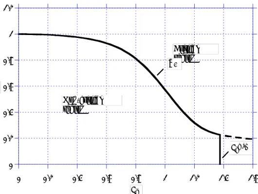
Figure 2.1. Diagram for fracture assessment (FAD). 0 0.2 0.4 0.6 0.8 1 1.2 0 0.2 0.4 0.6 0.8 1 1.2 1.4 1.6 Critical region fR6 Non-critical region Lrmax Lr Kr SSM 2008:01 16
The non-critical region is limited by,
2 6
6 (1 0.14 )[0.3 0.7 exp( 0.65 )] ,
r R r r
K £ f = - L + - L (2.1)
1, for materials with a yield plateu . , for all other cases
max f r r Y L L s s ì ï £ = í ï î (2.2)
10) Assessment of results (Chapter 2.11).
2.2 Characterization of defect
A fracture mechanics analysis requires that the actual defect geometry is characterized in a unique manner. For application to components in nuclear power facilities methods according to Appendix A should be used to define shape and size of cracks.
For assessment of an actual defect it is important to determine whether the defect remains from the manufacture or has occurred because of service induced processes such as fatigue or stress corrosion cracking.
2.3 Choice of geometry
The geometries considered in this procedure are documented in Appendix G. In the idealization process from the real geometry to these cases care should be taken to avoid non-conservatism. In cases when an idealization of the real geometry to one of the cases considered here are not adequate, stress intensity factor and limit load solutions can be found in the literature or be calculated by numerical methods. The use of such solutions should be carefully checked for accuracy.
2.4 Stress state
In this procedure it is assumed that the stresses have been obtained under the assumption of linearly elastic material behaviour. The term nominal stress denotes the stress state that would act at the plane of the crack in the corresponding crack free component.
The stresses are divided into primary s and secondary p s stresses. Primary stresses are caused s
by the part of the loading that contributes to plastic collapse e.g. pressure, gravity loading etc. Secondary stresses are caused by the part of the loading that does not contribute to plastic collapse e.g. stresses caused by thermal gradients, weld residual stresses etc. If the component is cladded this should be taken into account when the stresses are determined.
All stresses acting in the component shall be considered. The stresses caused by the service conditions should be calculated according to some reliable method. Some guidance about weld residual stresses is given in Appendix R.
2.5 Material data
To perform the assessments the yield strength s , the ultimate tensile strength Y s , the critical U stress intensity factor K and cr J -curves of the material must be determined. If possible, data r
obtained from testing of the actual material of the component should be used. This is not always possible and therefore minimum values for s and Y s from codes, standards or material U specifications may be used. These data should be determined at the actual temperature.
Y
s is equal to the lower yield strength R if this can be determined and in other cases the 0.2% eL
proof stress Rp0,2. In the cases when R can be determined the material is considered to have a eL
yield plateau. This is for instance common for certain low alloy carbon manganese steels at low temperatures.
U
s is the ultimate tensile strength of the material.
The yield strength and ultimate tensile strength of the base material should normally be used even when the crack is situated in a welded joint. The reason for this is that the yield limit of the structure is not a local property but also depends on the strength properties of the material remote from the crack.
cr
K is the critical value of the stress intensity factor for the material at the crack front. If
possible, K should be set equal to the fracture toughness cr K according to ASTM E399 [2.1]. Ic
It is in many cases not possible to obtain a valid K -value. Ic J -values according to ASTM Ic
E1820 [2.2] can be used instead and be converted according to Eq. (2.3).
I 2 . 1 c cr EJ K n = - (2.3) SSM 2008:01 18
Here E is the elastic modulus of the material and n is Poisson’s ratio.
Ductile materials normally show a significant raise of the J-resistance curve after initiation. When taking this into account, J -data according to ASTM E1820 [2.2] should be used. r
For application on nuclear components fracture toughness and J -curves according to Appendix r
M can be used if actual test data for the considered material is not available.
When not stated otherwise the material data for the actual temperature should be used.
2.6 Calculation of slow crack growth
The final fracture assessment as described below should be based on the estimated crack size at the end of the service period. In cases where slow crack growth due to fatigue, stress corrosion cracking or some other mechanism can occur the possible growth must be accounted for in the determination of the final crack size.
The rate of crack growth due to both fatigue and stress corrosion cracking is supposed to be governed by the stress intensity factor K . This quantity is calculated according to methods I
described in Appendix K.
For fatigue crack growth, the rate of growth per loading cycle can be described by an expression of the form I ( , ) . f da g K R dN = D (2.4) Here I I I , max min K K K D = - (2.5) and I I , min max K R K = (2.6) SSM 2008:01 19
where KImax and
Imin
K are the algebraic maximum and minimum, respectively, of K during the I
load cycle. g is a material function that can also depend on environmental factors such as f
temperature and humidity. For cases when R < 0 the influence of the R-value on the crack growth rate can be estimated by use of growth data for R = 0 and an effective stress intensity factor range according to
I I , if I 0 .
eff max min
K K K
D = < (2.7)
For application on nuclear components fatigue crack growth data according to Appendix M can be used if actual test data for the considered material is not available.
For stress corrosion cracking, the growth rate per time unit can be described by a relation of the form I ( ) . sc da g K dt = (2.8) sc
g is a material function which is strongly dependent on environmental factors such as the
temperature and the chemical properties of the environment.
For application on nuclear components stress corrosion crack growth data according to Appendix M can be used if actual test data for the material and environment under consideration is not available.
2.7 Calculation of K and Ip
Is
K
The stress intensity factors K (caused by primary stresses Ip s ) and p
I
s
K (caused by secondary
stresses s ) are calculated with the methods given in Appendix K. For the cases given it is s
assumed that the nominal stress distribution (i.e. without consideration of the crack) is known. Limits for the applicability of the solutions are given for the different cases. If results are desired for a situation outside the applicability limits a recharacterization of the crack geometry can sometimes be made. The following recharacterizations are recommended:
a) A semi-elliptical surface crack with a length/depth ratio which is larger than the applicability limit can instead be treated as an infinitely long two-dimensional crack. b) A semi-elliptical surface crack with a depth that exceeds the applicability limit can instead
be treated as a through-thickness crack with the same length as the original crack.
c) A cylinder with a ratio between wall thickness and inner radius which is below the applicability limit can instead be treated as a plate with a corresponding stress state.
In cases when the solutions of Appendix K cannot be applied, stress intensity factors can be obtained either by use of solutions found in the literature, see for example the handbooks [2.3], [2.4], [2.5] and [2.6], or by numerical calculations, e.g. by the finite element method.
2.8 Calculation of L r
r
L is defined as the ratio between the current primary load and the limit load P for the L
component under consideration and with the presence of the crack taken into account. P should L
be calculated under the assumption of a perfectly-plastic material with the yield strength s Y chosen as discussed in Chapter 2.5. Appendix L contains solutions of L for the cases considered r
in this procedure.
Limits for the applicability of the solutions are given for the different cases. If results are desired for a situation outside the applicability limits a recharacterization of the crack geometry can sometimes be made similarly to what was discussed for the stress intensity factor above.
In cases when the solutions of Appendix L cannot be applied, L can be obtained either by use r
of solutions found in the literature, see for example [2.7], or by numerical calculations, e.g. by the finite element method.
2.9 Calculation of K r
The ordinate K in the failure assessment diagram (Fig. 2.1) is calculated in the following way. r
I I , p s r cr K K K K r + = + (2.9)
where r is a parameter that takes into account plastic effects because of interaction between secondary and primary stresses. r is obtained from the diagram in Fig. 2.2 where r is given as a function of L and the parameter r c defined as
I I . s r p K L K c = (2.10)
c is set to zero if c falls below zero. Also, r is restricted to non-negative values as defined in
Fig. 2.2.
Figure 2.2. Diagram for calculation of r .
2.10 Fracture assessment
In order to assess the risk of fracture the assessment point
(
L K calculated as described above r, r)
is plotted in the diagram in Fig. 2.1. If the point is situated within the non-critical region no initiation of crack growth is assumed to occur and thus no fracture. The non-critical region is limited by the R6 option 1 (see R6, Revision 3 or [2.8]) type failure assessment curve according to 2 6 6 (1 0.14 )[0.3 0.7 exp( 0.65 )] , r R r r K £ f = - L + - L (2.11) . max r r L £L (2.12) 0 0.05 0.1 0.15 0.2 0.25 0 0.2 0.4 0.6 0.8 1 1.2 1.4 0.25 0.5 0.75 1 1.5 2 3 4 > 5.2 c r L r SSM 2008:01 22For materials which shows a continuous stress-strain curve without any yield plateau, the upper limit of L is defined by r , f max r Y L s s = (2.13)
where s is the uniaxial flow stress. Depending on application and type of material, f s is given f by
2.4 , for ferritic nuclear components
3.0 , for austenitic nuclear components .
( ) / 2, for all other cases
m f m Y U S S s s s ì ï = í ï + î (2.14)
Here S is the allowable design stress defined by m
(20 C) ( ) 2 (20 C) 2 ( ) min , , , , 3 3 3 3 U U Y Y m T T S = æç s s s s ö÷ è ø o o (2.15)
for ferritic materials and by
(20 C) ( ) 2 (20 C) min , 0.9 ( ), , , 3 3 3 U U Y m Y T S = æç s s T s s ö÷ è ø o o (2.16)
for austenitic materials. T is the temperature of the material. For materials that exhibit a discontinuous yield point max
r
L is restricted to 1.0. This is
conservative and should be regarded as a compromise when applying the option 1 type R6 failure assessment curve to a problem that is actually better described by an option 2 type failure assessment curve, cf. [2.8].
When the failure load of a component with a crack is sought, the above described procedure is carried out for different load levels and the crack geometry is kept constant. The critical load is then given by the load level which causes the point
(
L K to fall on the border to the critical r, r)
region. Similarly, the limiting crack size is obtained by keeping the loads fixed and calculating the point(
L K for different crack sizes until it falls on the border to the critical region. r, r)
In order to assess the risk of fracture for materials with high toughness, stable crack growth has to be included in the assessment. The non-critical region is here limited by
, R J =J (2.17) , app R T £T (2.18)
where J is the applied J, J is the resistance curve, R T is the applied tearing modulus and app T is R
the tearing modulus. In Appendix B, the background to this assessment is given.
2.11 Safety assessment
The following conditions should be fulfilled to determine if a detected crack of a certain size is acceptable, cf. [2.9]: Ic , J J J SF £ (2.19) . L L P P SF £ (2.20)
Eqs. (2.19) and (2.20) account for the failure mechanisms fracture and plastic collapse and SF J
and SF are the respective safety factors against these failure mechanisms. Plastic collapse is L
assumed to occur when the primary load P is equal to the limit load P . This occurs when the L
remaining ligament of the cracked section becomes fully plastic and has reached the flow stress
f
s . J is the path-independent J-integral which is meaningful for situations where J completely
characterizes the crack-tip conditions. J should be evaluated with all stresses present (including residual stresses) and for the actual material data. J is the value of the J-integral at which Ic
initiation of crack growth occurs.
In this procedure J is estimated using the option 1 type R6 failure assessment curve [2.8]. The R6-estimation of J is given by 2 2 I 2 6 (1 ) 1 , [ R ( )r ] K J E f L n r -= - (2.21) SSM 2008:01 24
where f is defined by Eq. (2.11). The second fraction on the right hand side of Eq. (2.21) can R6
be interpreted as a plasticity correction function, based on the limit load, for the linear elastic value of J determined by the stress intensity factor K . I
Combining Eqs. (2.3), (2.19) and (2.21) gives the following relation for the acceptance of a crack: 6 I R ( )r . cr J J f L K K SF SF r + £ (2.22)
The left-hand side of Eq. (2.22) represents the parameter K used for safety assessment. Eq. r
(2.22) implies that the assessment point
(
L K should be located below the R6 failure r, r)
assessment curve divided by the safety factor SF . The maximum acceptable condition is Jobtained in the limit when the assessment point is located on the reduced failure assessment curve, expressed by Eq. (2.22) with a sign of equality. In addition a safety factor against plastic collapse, corresponding to Eq. (2.19), is introduced as a safety margin against the cut-off of L r
as . max r r L L L SF £ (2.23)
Eqs. (2.22) and (2.23) represent the safety assessment procedure used in this handbook and in the PC-program ProSACC [2.10]. In Appendix S, a set of safety factors are defined to be used for nuclear applications, cf. [2.9]. The safety factor SF is introduced which is the safety factor on K
cr
K corresponding to the safety factor SF on J J . They are related through Ic SFK = SFJ .
Critical conditions are obtained when all safety factors are set to unity and when the assessment point is located on the failure assessment curve.
One drawback with this deterministic safety evaluation system is that it may overestimate the contribution from secondary stresses (i.e. welding residual stresses or stresses from a thermal transient) for ductile materials. The Swedish Nuclear Power Inspectorate and Det Norske Veritas has therefore started a project that will lead to a quantitative recommendation on how to treat secondary stresses for high L -values in a R6 fracture assessment. This recommendation will r
define new safety factors against fracture described by K and differentiate between I Primary K
SF
(relating to primary stresses) and Secondary K
SF (relating to secondary stresses). The results from this project will be incorporated in the next revision of the handbook.
Ductile materials normally show a significant raise of the J-resistance curve after initiation. When doing a safety assessment, including stable crack growth, Eq. (2.19) is no longer valid. The acceptable region is then given by
and . R R app J J J T J T SF SF £ £ (2.24)
In cases which are particularly difficult to assess, a sensitivity analysis may be necessary. Such an analysis is simplest to perform by a systematic variation of the load, crack size and material properties.
2.12 References
[2.1] —, (1997), “Standard Test Method for Plane-Strain Fracture Toughness of Metallic Materials”, ASTM Standard E399 – 90.
[2.2] —, (2001), “Standard Test Method for Measurement of Fracture Toughness”, ASTM Standard E 1820 – 01.
[2.3] MURAKAMI, Y. (ed.), (1987-1991), Stress intensity factors handbook, Vol. 1-3, Pergamon Press, Oxford, U.K.
[2.4] MURAKAMI, Y. (ed.), (2001), Stress intensity factors handbook, Vol. 4-5, Elsevier, Oxford, U.K.
[2.5] TADA, H., PARIS, P. C., and G. C. IRWIN, (1985), The stress analysis of cracks
handbook, 2nd edition, Paris Productions Inc., St. Louis, U.S.A.
[2.6] ROOKE, D. P., and D. J. CARTWRIGHT, (1976), Compendium of stress intensity
factors, Her Majesty’s Stationary Office, London, U.K.
[2.7] MILLER, A. G., (1988), “Review of limit loads of structures containing defects”, The
International Journal of Pressure Vessels and Piping, Vol. 32, pp. 197-327.
[2.8] MILNE, I., AINSWORTH, R. A., DOWLING, A. R., and A. T. STEWART, (1988), “Assessment of the integrity of structures containing defects”, The International
Journal of Pressure Vessels and Piping, Vol. 32, pp. 3-104.
[2.9] BRICKSTAD, B., and M. BERGMAN, (1996), “Development of safety factors to be used for evaluation of cracked nuclear components”, SAQ/FoU-Report 96/07, SAQ Kontroll AB, Stockholm, Sweden.
[2.10] DILLSTRÖM, P., and W. ZANG., (2004), “User manual ProSACC Version 1.0”, DNV Research Report 2004/02, Det Norske Veritas AB, Stockholm, Sweden.
TABLE OF REVISIONS
Rev Activity / Purpose of this revision Handled by Date
4-1 First printing of revision 4 of the handbook. Peter Dillström 2004-10-14
APPENDIX A. DEFECT CHARACTERIZATION
A fracture mechanics assessment requires that the current defect geometry is characterized uniquely. In this appendix general rules for this are given. For additional information it is referred to ASME Boiler and Pressure Vessel Code, Sect. XI [A1].
A1. Defect geometry
Surface defects are characterized as semi-elliptical cracks. Embedded defects are characterized as elliptical cracks. Through thickness defects are characterized as rectangular cracks. The characterizing parameters of the crack are defined as follows:
a) The depth of a surface crack a corresponding to half of the minor axis of the ellipse. b) The depth of an embedded crack 2a corresponding to the minor axis of the ellipse. c) The length of a crack l corresponding to the major axis of the ellipse for surface and
embedded cracks or the side of the rectangle for through thickness cracks.
In case the plane of the defect does not coincide with a plane normal to a principal stress direction, the defect shall be projected on to normal planes of each principal stress direction. The one of these projections is chosen for the assessment that gives the most conservative result according to this procedure.
A2. Interaction between neighbouring defects
When a defect is situated near a free surface or is close to other defects the interaction shall be taken into account. Some cases of practical importance are illustrated in Fig. A1. According to the present rules the defects shall be regarded as one compound defect if the distance s satisfies the condition given in the figure. The compound defect size is determined by the length and depth of the geometry described above which circumscribes the defects. The following shall be noted:
a) The ratio l/a shall be greater than or equal to 2.
b) In case of surface cracks in cladded surfaces the crack depth should be measured from the free surface of the cladding. If the defect is wholly contained in the cladding the need of an assessment has to be judged on a case-by-case basis.
c) Defects in parallel planes should be regarded as situated in a common plane if the distance between their respective planes is less than 12.7 mm.
Case Defect sketches Criterion 1 s 2a1 If s < 0.4a1 then a = 2a1 + s 2 l1 s l2 If s < min(l1, l2) then l = l1 + l2 + s 3 s l2 l1 If s < min(l1, l2) then l = l1 + l2 + s 4 s 2a1 2a2 If s < max(2a1, 2a2) then 2a = 2a1 + 2a2 + s 5 s 2a1 a2 If s < max(2a1, a2) then a = 2a1 + a2 + s 6 2a1 a2 l2 s1 l1 s2 If s1 < max(2a1, a2) and s2 < min(l1, l2) then a = 2a1 + a2 + s1 l = l1 + l2 + s2
Figure A1. Rules for defect characterization at interaction.
A3. References
[A1] —, (1995), ASME Boiler and Pressure Vessel Code, Sect. XI, Rules for inservice
inspection of nuclear power plant components. The American Society of Mechanical
Engineers, New York, U.S.A.
APPENDIX R. RESIDUAL STRESSES
Residual stresses are defined as stresses existing in a structure when it is free from external loading. The distribution and magnitude of residual stresses in a component depend on the fabrication process and service influences. Residual stresses are normally created during the manufacturing stage but can also appear or be redistributed during service. At pressure or load test of a component, peaks of residual stresses can be relaxed due to local plasticity if the total stress level exceeds the yield strength of the material.
It is anticipated that with increasing amount of external load (increasing limit load parameter L ) r
the contribution to the risk of fracture from the weld residual stresses is diminished. There is experimental evidence [R1], which demonstrates that for ductile materials, the influence of weld residual stresses on the load carrying capacity is quite low. In [R1] the influence of the weld residual stresses beyond L of 1.0 was almost zero. The ASME Code, Section XI, has dealt with r
this problem by simply ignoring weld residual stresses for certain materials, for instance for austenitic stainless steels. However, this treatment is questionable for situations that is dominated by secondary loads (e.g. for thermal shock loads) and when the material is not sufficiently ductile that the failure mechanism is controlled only by plastic collapse. The Swedish Nuclear Power Inspectorate and Det Norske Veritas has therefore started a project that will lead to a quantitative recommendation on how to treat weld residual stresses for high L -values in a R6 r
fracture assessment. The results from this project will be incorporated in the next revision of the handbook.
Guidelines for estimation of residual stresses in steel components due to welding are given below for use in cases when more precise information is not available. In some cases, welding leads to formation of bainite or martensite at cooling which results in a change in volume. Such a volume change affects the weld residual stresses and makes it difficult to perform accurate predictions. A more comprehensive compendium of residual stress profiles are given in [R2-R4]. The residual stresses are given in the transverse and longitudinal directions, corresponding to stresses normal and parallel to the weld run. Weld residual stresses acting in the through thickness direction are assumed to be negligible.
The magnitude of the residual stresses are expressed in S which is set to the 0.2% yield strength r
of the material at the actual temperature, see Chapter 2.5. For austenitic stainless steels, however,
r
S should be chosen to the 1% proof stress at the considered temperature. This is mainly due to
the large strain hardening that occurs for stainless steels. If data for the 1% proof stress is missing, it may be estimated as 1.3 times the 0.2% proof stress. The actual yield strength values rather than minimum values should be used for a realistic estimation.
For an overmatched weld joint, the yield strength is referred to the weld material for the residual stress in the longitudinal direction in the weld centerline. For the transverse residual stress, the yield strength is in general referred to the base material.
R1. Butt welded joints
R1.1 Thin plates
With thin plates is here meant plates with butt welds where the variation of the residual stress in the thickness direction is insignificant. This holds for butt welds with only one or a few weld beads.
The weld residual stresses acting in the longitudinal direction of the weld has a distribution across the weld according to Fig. R1. The width of the zone with tensile stresses l is about four to six times the plate thickness. This distribution is obtained along the entire weld except when the weld ends at a free surface where the stresses tend to zero.
Figure R1. Distribution across the weld of residual stresses acting in the longitudinal direction of the weld.
The magnitude of the weld residual stresses acting transverse to the weld direction is dependent on whether the plates have been free or fixed during welding. If for instance, the plates are fixed to each other by tack welding before the final welding, residual stresses with a magnitude up to
r
S are obtained. If one of the two plates is free to move during cooling the residual stresses
become limited to 0.2S , see e.g. Ref. [R5]. The values are valid at the centerline of the weld. r
They successively diminish in sections outside the centerline. -0.5 0 0.5 1 1.5 -2 -1.5 -1 -0.5 0 0.5 1 1.5 2 s / Sr x / l SSM 2008:01 34
R1.2 Thick plates
In thick plates welded with many weld beads the variation of the residual stresses in the thickness direction cannot be neglected. The stress distribution is much more complicated in thick plates than in thin plates and depends very much on joint design and weld method. It is therefore difficult to give simple general guidelines for estimation of residual stresses in thick plates. It is not possible to give a specific value of the plate thickness that represents the transition from a thin to a thick plate. For more detailed information, see Refs. [R2, R6-R8]. The weld residual stresses acting in the weld vary both in the thickness direction and across the weld. The highest stress in the symmetry plane of the weld is S . The simplest but in many cases r
very conservative assumption is that the weld residual stress is constant and equal to S r
throughout the entire thickness.
In a symmetric joint, for instance an X-joint or a double U-joint with many weld beads, the residual stress through the thickness t varies as shown in Fig. R2.
Figure R2. Thickness distribution of residual stresses acting in a welded thick plate in a symmetric joint with many weld beads. This distribution for residual stresses acting transverse the weld applies for a free plate.
-1.5 -1 -0.5 0 0.5 1 1.5 -0.5 -0.25 0 0.25 0.5 s / Sr x / t Transverse stress Longitudinal stress SSM 2008:01 35
The weld residual stresses acting transverse the weld vary as shown in Fig. R2 if any of the plates is free to move during the cooling.
R1.3 Butt welded pipes
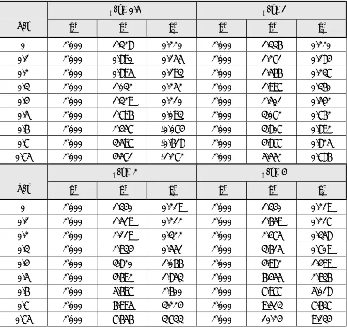
The residual stress distribution in girth welds in both thick walled and thin walled pipes are complicated and depends on joint shape, weld method, heat input, wall thickness and pipe radius. The recommendations given here are based on a numerical investigation on austenitic stainless steel pipes [R9] and apply to girth welds applied from the outside (single sided V- or U-preparation). They are valid for a radius to thickness ratio R t of approximately 8 but can i/ conservatively be used for higher ratios of R t . The heat input relative to the pipe thickness i/ was between 75 and 101 MJ/m2 which is considered to be high. More detailed information is given in [R9]. A parametric study of a large number of pipes can also be found in [R10].
The local residual stresses acting longitudinal and transverse to a girth weld are shown in Fig. R3 for a pipe thickness up to 30 mm. The stresses decrease successively in sections further outside the fusion line.
t Ri -1 1 x 1 x s / sm s / sb
Figure R3. Local distribution of residual stress acting longitudinal and transverse to a girth weld for an austenitic pipe up to a thickness of 30 mm.
In Table R1 the specific values of the membrane stress s and local bending stress m s are b
given. They are taken from [R9] and determined at 288 °C which is a common operating temperature for nuclear LWR plants.
The local residual stresses acting longitudinal and transverse to a girth weld are shown in Fig. R4, for a pipe thickness greater than 30 mm. The stresses decrease successively in sections further outside the fusion line.
t Ri 1 1 x x s / sm s / s0 s = s0[1.0+ 3.8116 x t( )- 99.820 x t( )2 + +339.97 x t( )3- 404.59 x t( )4+ 158.16 x t( )5 ] Figure R4. Local distribution of residual stress acting longitudinal and transverse to a girth weld
for an austenitic pipe with a thickness greater than 30 mm.
In Table R1 the specific values of the membrane stress s and stress amplitude m s are given. 0
They are determined at 288 °C.
In [R9] the stainless steel pipes considered were overmatched with a weld material yield strength at 1% strain of 348 MPa and base material yield strength at 1% strain of 187 MPa at 288 °C. S r
in Table R1 is referred to the 1% proof stress at 288 °C for the base material except for the longitudinal stress at the weld centerline where S is referred to the 1% proof stress of the weld r
material. For other combinations of weld and base material yield properties, appropriate adjustments of these recommendations can be made according to Table R1.
Pipes with a thickness up to 40 mm were studied in [R9]. For a pipe wall thickness greater than this, the recommendations in Table R1 should be conservative.
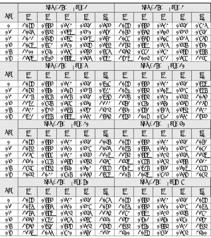
Table R1. Recommended longitudinal and transverse residual stress distributions for austenitic stainless steel pipe welds at 288 °C. x = 0 at the inside of the pipe wall. See Figs. R3 and R4.
Transverse stress [MPa]
t [mm] Weld centerline and HAZ
7 t£ 1.219S [1 - 2( /r x t )] 7< £t 25 (1.5884 - 0.05284t) S [1 - 2( /r x t )] 25< £t 30 0.2674S [1 - 2( /r x t )] 30 t > 0.4246S [1 + 3.8116( /r x t ) - 99.82( /x t )2 + 339.97( /x t )3 - 404.59( /x t )4 + 158.16( /x t )5]
Longitudinal stress [MPa]
t [mm] Weld centerline HAZ
30
t£ 0.925Sr 0.861Sr
30
t > 0.925S r 0.646S r
For ferritic steel piping, predictions based on numerical methods are more difficult due to volume changes during certain phase transformations. Based on the investigation in [R10], the principal feature for the residual stresses for girth welds should be similar as for austenitic piping. Thus if no other data for a specific case exists, it is proposed to use Table R1 also for ferritic piping. Proper adjustment has to be made for the actual yield properties of the ferritic pipe weld. Also, the bending stress s for thinner pipes in Table R1, should be limited to the b
yield strength for a ferritic pipe.
R1.4 Butt-welded bimetallic pipes (V or U shape)
The recommendations of the residual stress distribution given here are based on a numerical investigation [R3-R4] and apply to girth welds applied from the outside (single sided V- or U-preparation), see Fig. R5. It is shown that the material at HAZ has little influence on residual stress. The position (left or right) decides the magnitude and the distribution of the residual stress.
Weld type (a)
Alloy 182
HAZ-left Weld centerline HAZ-right
Alloy 600 Carbon steel Stainless steel Alloy 182 Weld type (b) Alloy 182
HAZ-left Weld centerline HAZ-right
Stainless steel Carbon steel Stainless steel Alloy 182 Weld type (c) Alloy 182
HAZ-left Weld centerline HAZ-right
Stainless steel Carbon steel
Stainless steel
Weld type (d)
Stainless steel Alloy 182 Alloy 600
HAZ-left Weld centerline HAZ-right
Figure R5. Butt-welded bimetallic pipes (single sided V- or U-preparation).
The weld residual stress across the thickness is fitted by a 5-th degree polynomial as, 5 0 1 i i i u c c t s = ì ü ï æ ö ï =í + ç ÷ ý è ø ï ï î
å
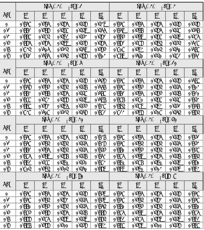
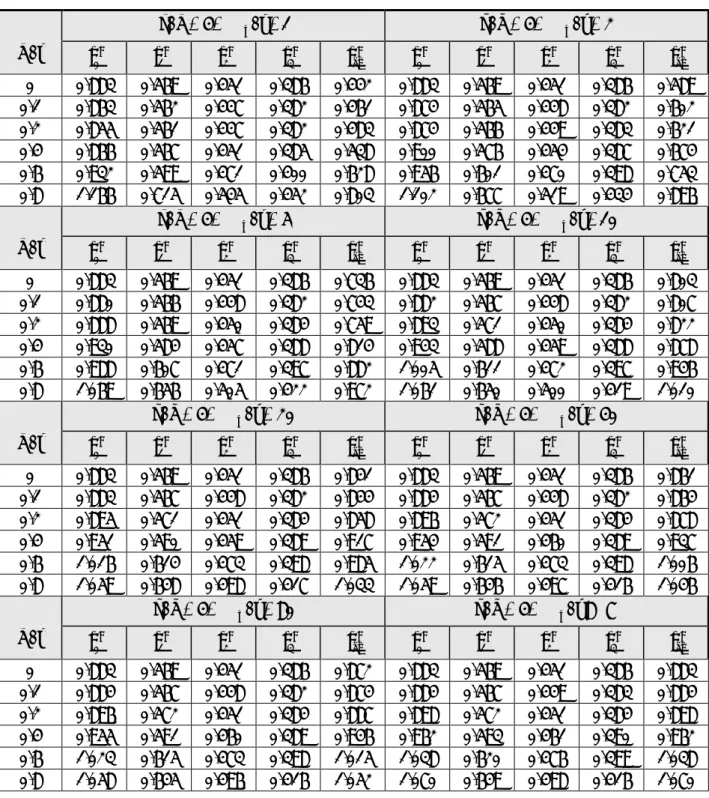
þ MPa , (R1)where u = 0 indicates the inside surface of the pipe and t the thickness of the pipe. The parameters for the recommended weld residual stresses are presented in Tables R2 and R3 at three different cross lines, namely at the weld centre line, the HAZ left line and the HAZ right line. The stress distributions are also plotted in Fig. R6 and R7.
Table R2. Recommended transverse residual stress for butt-welded bimetallic pipes.
Position t [mm] c 0 c 1 c 2 c 3 c 4 c 5 HAZ left 245.0 539.8 -5734.5 12197. -11190. 3849.1 Weld centre 171.2 1257.6 -7048.2 11265. -8498.5 2570.4 HAZ right t < 10 253.4 188.3 -4357.1 7951.5 -5555.0 1396.4 HAZ left 129.3 26.2 -2066.3 7944.4 -11395. 5175.9 Weld centre 124.1 934.6 -9166.4 24979. -28074. 11005. HAZ right 10 < t ≤ ≤ 20 149.9 -800.3 1694.4 -2322.8 1724.8 -477.1 HAZ left 52.4 66.6 -5063.3 21002. -28115. 11925. Weld centre 100.7 -50.1 -5156.3 18102. -20949. 7833.0 HAZ right 20 < t ≤ ≤ 30 140.2 -1192.8 1868.0 1848.7 -6318.7 3782.3 HAZ left 33.0 -466.4 -4326.5 21424. -27647. 10915. Weld centre 32.9 -177.4 -5280.1 20579. -24143. 8986.1 HAZ right 30 < t ≤ ≤ 70 102.3 -1682.4 4191.1 -610.9 -6619.8 4881.2 SSM 2008:01 40
-300 -200 -100 0 100 200 300 0 0,2 0,4 0,6 0,8 1 HAZ left (0 < t < 10) Weld centre (0 < t < 10) HAZ right (0 < t < 10) Stress [MPa] u/t -300 -200 -100 0 100 200 300 0 0,2 0,4 0,6 0,8 1 HAZ left (10 < t < 20) HAZ right (10 < t < 20) Weld centre (10 < t < 20) Stress [MPa] u/t -300 -200 -100 0 100 200 300 0 0,2 0,4 0,6 0,8 1 HAZ left (20 < t < 30) Weld centre (20 < t < 30) HAZ right (20 < t < 30) Stress [MPa] u/t -300 -200 -100 0 100 200 300 0 0,2 0,4 0,6 0,8 1 HAZ left (30 < t < 70) Weld centre (30 < t < 70) HAZ right (30 < t < 70) Stress [MPa] u/t
Figure R6. Recommended transverse residual stress for butt-welded bimetallic pipes.
Table R3. Recommended longitudinal (hoop) residual stress for butt-welded bimetallic pipes. Position t [mm] c 0 c 1 c 2 c 3 c 4 c 5 HAZ left 187.9 38.7 107.8 -1831.0 1993.9 -512.8 Weld centre 371.6 451.6 -1071.9 -1044.7 2504.2 -1151.1 HAZ right t < 10 197.8 523.3 -806.1 -2881.9 5462.9 -2457.7 HAZ left 248.2 297.3 -1696.1 5125.5 -7120.0 3173.0 Weld centre 386.1 671.7 -6490.3 17792. -19862. 7662.3 HAZ right 10 < t ≤ ≤ 20 170.4 -315.5 1117.5 -1624.8 745.4 -14.3 HAZ left 252.2 -231.7 -354.8 5424.9 -9185.7 4174.3 Weld centre 172.5 -658.2 2458.6 -159.7 -3635.1 2046.1 HAZ right 20 < t ≤ ≤ 30 89.9 -596.9 4191.8 -6975.5 3644.5 242.7 HAZ left 16.4 -605.3 812.7 9426.8 -18206. 8689.4 Weld centre 88.7 170.4 -2984.4 13346. -17190. 6833.8 HAZ right 30 < t ≤ ≤ 70 91.9 273.8 -2184.1 11029. -16671. 7719.9 SSM 2008:01 42