The spatially-distributed AgroEcoSystem-Watershed (AgES-W)
hydrologic/water quality (H/WQ) model for assessment of conservation
effects
James C. Ascough II, Timothy R. Green, Gregory S. McMaster
USDA-ARS-PA, Agricultural Systems Research Unit, Fort Collins, CO, 80526 USA Olaf David, Holm Kipka
Colorado State University, Dept. of Civil and Environmental Engineering, Fort Collins, CO, 80523 USA
Abstract. AgroEcoSystem-Watershed (AgES-W) is a modular, Java-based spatially distributed model which implements hydrologic/water quality (H/WQ) simulation components under the Object Modeling System (OMS3) environmental modeling framework. AgES-W has recently been enhanced with the addition of nitrogen (N) and sediment modeling components refactored from various agroecosystem models including SWAT, WEPP, and RZWQM2. The specific objectives of this study are to: 1) present an overview of major AgES-W processes and simulation components; 2) evaluate the accuracy and applicability of the enhanced AgES-W model for estimation (using a newly developed autocalibration tool) of streamflow and N/sediment loading for the Upper Cedar Creek Watershed (UCCW) in northern Indiana, USA; and 3) discuss the efficacy of AgES-W for assessing spatially targeted agricultural conservation effects on water quantity and quality for the South Fork Watershed (SFW) in central Iowa, USA. AgES-W model performance was assessed using Nash-Sutcliffe model efficiency (ENS) and percent bias (PBIAS) model evaluation criteria.
Comparisons of simulated and observed daily and average monthly streamflow/N loading and monthly sediment load for different simulation periods resulted in ENS and PBIAS values that were
within the range of those reported in the literature for other H/WQ models at a similar scale and time step. Considering that AgES-W was applied with minimal calibration, study results indicate that the model reasonably reproduced the hydrological, N, and sediment dynamics of the target watersheds and should serve as a foundation upon which to better quantify additional water quality indicators (e.g., phosphorus dynamics) at the watershed scale.
1. Introduction
Since the mid-1980s, nonpoint source (NPS) pollution of streams, rivers, and other water bodies has been recognized as a major threat to water quality (Niraula et al. 2012). Although there are many potential contributors of NPS pollution, agriculture is the primary supplier of nutrients, pesticides, and sediment to streams and rivers in the United States (US EPA 2002). Agrochemicals and animal manures are extensively used in the U.S. to increase crop production, but their excessive or inappropriate application can cause serious water quality problems in both surface and groundwater resources. Many cropping system management practices, including application of nitrogen (N) fertilizer in various forms, provide a considerable source of nitrate (NO3-N) that may rapidly move to streams and
rivers through surface/subsurface flow or leach deeper into the soil profile and eventually reach groundwater systems in areas with susceptible soils and hydrogeology. Sediments not only contribute major chemical pollutants to surface water bodies but can also diminish the recreational and aesthetic values of the water. One area of the U.S. that experiences
persistent water quality problems due to overuse of agrochemicals is the Midwest Corn
Belt Region (CBR), one of the most productive agricultural regions in the world with nearly 80% of the U.S. corn and soybean production and more than 325,000 Mg of chemicals applied to cropland annually (Larose et al. 2007). There are many watersheds within the CBR that supply water to urban populations, including the Cedar Creek
Watershed (CCW) located in northeastern Indiana. The CCW is the largest tributary of the St. Joseph River, which supplies drinking water for approximately 250,000 people in the
city of Fort Wayne, Indiana. Over 50% of the CCW is under extensive corn (Zea mays L.)
and soybean (Glycine max (L.) Merr.) production, it is believed that most of the NPS pollution within the CCW is a result of chemical over-application within agricultural land use areas.
Effective management of intensely cropped watersheds like the CCW requires a broad understanding of hydrologic and chemical transport processes within the watershed
(Larose et al. 2007). When attempting to ameliorate problems caused by NPS pollution,
watershed managers need accurate and easily accessible data in order to make judicious decisions about management changes that could reduce levels of chemicals entering the water bodies under protection. The most direct and precise method for acquiring data in agricultural watersheds is by monitoring streamflow and water quality constituents. However, monitoring costs (i.e., instrumentation installation/maintenance, data collection, etc.) can be very expensive; furthermore, lack of understanding of hydrologic and chemical transport processes occurring within the watershed frequently result in misinterpretation of monitored data (Im et al. 2007). For these reasons, an appropriately selected watershed model, rigorously calibrated for the circumstances being investigated and used to predict the impact that variations in agricultural activities have on water quantity (runoff) and quality (nutrients, pesticides, and sediment), is indispensable for analyzing NPS pollution in agricultural watersheds. In recent years a number of physically-based simulation models have been developed to assess the effects of changes in land use, land cover, management practices, or climatic conditions on hydrology and water quality (H/WQ) at watershed scales. Examples of continuous watershed simulation models commonly reported in the literature include HSPF (Hydrologic Simulation Program), VIC (Variable Infiltration Capacity), ANSWERS-2000 (Areal Nonpoint Source Watershed Environment Response Simulation), AnnAGNPS (Annualized Agricultural Non-Point Source), PRMS
(Precipitation Runoff Modeling System), SWAT (Soil and Water Assessment Tool), and AgES-W (AgroEcoSystem-Watershed). These models generally operate on a daily time step, are computationally efficient, and often lump many comprehensive processes that occur over short time steps into simplifying approximations (Borah and Bera 2004). For the above models, the SWAT model is by far the most ubiquitous and has been applied to literally thousands of watersheds throughout the world (Gassman et al. 2007)
One distinguishing feature of the above models is the flow and chemical routing mechanism at the watershed scale. A noted historical shortcoming of SWAT is the
inability to model flow and transport from one landscape position to another prior to entry into the stream. The SWAT model utilizes a hydrologic response unit (HRU) concept where HRUs are lumped land areas within each sub-basin that are composed of unique land cover, soil, and management combinations. Transported runoff, chemicals, and sediment from HRUs within a sub-basin are currently routed directly into stream channel headwaters by SWAT, thereby circumventing lower landscape units. Thus, as currently configured, SWAT does not simulate flow and chemical transport from upstream HRUs to downstream HRUs prior to entering the stream. Conversely, the AgES-W and AnnAGNPS models are fully distributed, meaning that runoff, chemicals, and sediment are implicitly routed between individual land units. AgES-W model performance was previously
evaluated for CCW streamflow only (Ascough et al. 2012) and the model has recently been enhanced with the addition of: 1) detailed N and sediment dynamics process-based
component, and 3) a unique flow surface routing component that permits multi-dimensional linkage of HRU entities in such a way that each entity can have various (HRU) receivers to which water, chemicals, and sediment are passed. The overall goal of this study is to further advance the AgES-W development and evaluation effort using observed data from the Upper CCW (UCCW) sub-catchment of the CCW in northeastern Indiana, USA. Specific study objectives are to: 1) present an overview of major AgES-W processes, simulation components, and input/output file structure; 2) evaluate the accuracy and applicability of the enhanced AgES-W model for estimation (using a newly developed autocalibration tool) of streamflow and N/sediment loading for the Upper Cedar Creek Watershed (UCCW) in northern Indiana, USA; and 3) discuss the efficacy of AgES-W for assessing spatially targeted agricultural conservation effects on water quantity and quality for the South Fork Watershed (SFW) in central Iowa, USA.
2. Materials and Methods 2.1 Site description
The Cedar Creek watershed (CCW) is located within the St. Joseph River basin in northeastern Indiana, USA (41° 10' 10" to 41° 32' 38" N, 84° 53' 49" to 85° 19' 44" W) and covers Noble, DeKalb, and Allen counties. The CCW drains two 11-digit hydrologic unit code (HUC) sub-watersheds, Upper Cedar Creek (04100003080, Figure 1) and Lower Cedar Creek (04100003090), covering a total area of approximately 700 km2. The average land surface slope of the watershed is 2.6%, and topography varies from rolling hills to nearly level plains with minimum and maximum altitudes above sea level of 232 m and 326 m, respectively. Soil types on the watershed were formed from compacted glacial till, and the predominant soil textures are silt loam, silty clay loam, and clay loam (SJRWI 2004). The annual mean precipitation in the watershed area from 1989 to 2010 was 974 mm. The average temperature during crop growth seasons ranges from 10°C to 23°C. The watershed is mainly used for farmland and livestock production and is characterized by a high percentage of rotationally tilled agricultural row crops (~50%), grassland (~27%), woodland (~12%), and pasture (~8%).
2.2 AgES-W model description
AgES-W is a modular, Java-based spatially distributed model which implements H/WQ processes as encapsulated simulation components under the Object Modeling System Version 3 (OMS3, David et al. 2013). OMS3 is a framework for environmental model development that provides a consistent and efficient way to: 1) create science simulation components; 2) develop, parameterize, and evaluate environmental models and modify/adjust them as science advances; and 3) re-purpose environmental models for emerging customer requirements. OMS is an open source software project (i.e., all framework code is freely available at http://www.javaforge.com/project/oms) enabling members of the scientific community to collaborate to address complex issues associated with the design, development, and application of environmental models. The OMS
architecture has been designed so that it is interoperable with other frameworks supporting environmental modeling globally (David et al. 2013).
Figure 1. Upper CCW stream network and gauging stations.
AgES-W operates at various temporal (either hourly or daily time steps) and spatial aggregation levels throughout the watershed (Ascough et al. 2012). The generation of four separate runoff/N components, i.e., RD1 -- surface runoff, RD2 -- interflow from the unsaturated soil zone, RG1 -- interflow from the saturated zone of the underlying
hydrogeological unit, and RG2 -- saturated groundwater baseflow, is based on the J2K-SN model (Fink et al. 2007) and simulated inside the central modeling core of AgES-W for each HRU (Figure 2). Calculation of runoff, N, and sediment routing is performed using a lateral routing scheme with subsequent transport from HRUs into the stream channel network. The following sections describe AgES-W components of interest in this study including management, plant growth, N dynamics, sediment dynamics, and routing components for runoff, N, and sediment. AgES-W plant interception, evapotranspiration (ET), and soil water processes components were explained in detail in Ascough et al. (2012)and are presented only briefly herein.
2.2.1 Soil water module. The AgES-W soil water balance module is the central
component of the model and interacts with nearly all other AgES-W process modules. A schematic of the soil water balance module is shown in Figure 2. AgES-W first calculates interception storage (based on the leaf area index of the respective land use) and snow accumulation/melt. Infiltration into the soil profile is calculated next with surface runoff flow (RD1) generated (after accounting for surface depression storage) as a result of infiltration excess (Horton-type runoff) during high intensity rainfall or saturation excess (Dunne-type runoff). AgES-W has a unique storage water concept based on two
unsaturated zone soil compartments (Figure 2): 1) middle pore storage (MPS, mm d-1), analogous to the useable field capacity of the soil, in which stored water is held in middle-sized pores (diameter = 0.2-50 µm) against gravity and can only be drained by active tension; and 2) large pore storage (LPS, mm d-1), analogous to the air capacity of the soil in which large pores and macropores (diameter > 50 µm) are not able to hold water against gravity and are thus the primary source for vertical and horizontal outflows. In AgES-W, the MPS and LPS pore volumes are calculated for each soil layer using various soil physical properties. For each soil layer, the specific values of the large pore volume of the entire layer depth are summed providing the maximum LPS storage capacity. For the MPS, only middle pore volumes of the soil horizons lying in the range of the effective rooting depth are considered. The groundwater (aquifer) domain is conceptualized by the RG1 and RG2 storages for each HRU (Figure 2). RG1 represents the (faster) water movement in the shallow bedrock weathering zone and RG2 represents the (slower) water movement in the deeper aquifer and/or in fractures and is equivalent to baseflow. Percolation from the LPS into the groundwater module is distributed among the RG1 and RG2 storages based on slope and an empirical calibration parameter. Outflow from the RG1 and RG2 storages is calculated from the actual storage content, a groundwater recession coefficient, and another empirical calibration parameter.
2.2.2 Plant growth and management modules. The AgES-W plant growth component
model (Figure 3) is a simplified version of the SWAT plant growth module (Neitsch et al. 2011). It computes potential plant growth, i.e., plant growth under optimal conditions (adequate water, nutrient supply, and favorable climatic environments) which is then modified in consideration of water, temperature, and nutrient stresses. Differences in growth between plant species are defined by the parameters contained in the plant parameter database (also derived from SWAT). Plant growth is simulated by computing leaf area development from light interception and its conversion to biomass. AgES-W land
use management (Figure 3) operations include planting, harvesting, tillage, and fertilizer application. Information required in the plant operation includes the timing of the operation (month and day or fraction of base zero potential heat units), the total number of heat units required for the land cover to reach maturity, and the specific land cover to be simulated in the HRU. The only information required by the harvest operation is the date; however, a harvest index override and a harvest efficiency can be set. The tillage operation
redistributes residue and nutrients in the soil profile and modifies soil physical properties (e.g., bulk density) based on tillage implement type and tillage depth. Information required in the tillage operation includes the timing of the operation (month and day or fraction of base zero potential heat units), and the type of tillage operation. The fertilizer operation applies fertilizer or manure to the soil. Information required in the fertilizer operation includes the timing of the operation (month and day or fraction of plant potential heat units), the type and amount of fertilizer/manure applied, and the depth distribution of fertilizer application.
Figure 3. Conceptual hydrologic and nitrogen (N) components of AgES-W coupled with land use management and crop growth components.
2.2.3 N dynamics module. The AgES-W N dynamics module is loosely based on the
SWAT model N component (Neitsch et al. 2011). Within the individual soil layers, five N pools for NO3-N, ammonium (NH4-N), stable organic substances, active organic
substances, and fresh plant residue as biomass are distinguished. These are initialized separately in order to provide stable pools at the beginning of model simulation. The fluxes and transformations between the pools and outside the soil (e.g., nitrification,
relationships in conjunction with the soil moisture and temperature. Soil temperature (Figure 3) is modeled in AgES-W as a modified version of the empirical soil temperature routines found in the SWAT and EPIC models and is a function of previous day soil temperature, the average annual air temperature, the current day soil surface temperature, and the depth in the soil profile. Initially, a surface soil temperature is generated for bare ground on the basis of the air temperature and insolation and is modified by attenuation factors that describe the effect of biomass and snow. The temperature of the different soil horizons is generated as an upper boundary condition between the surface soil temperature and the long-term mean temperature as a lower boundary condition. The attenuation effect of the soil is defined in consideration of the soil humidity and the bulk density. General equations for the individual processes can be found in Neitsch et al. (2011).
2.2.4 Sediment transport dynamics module. The AgES-W sediment module implements
the Modified Universal Soil Loss Equation (MUSLE) as described in Williams (1995) as:
(
Q q area)
K C P LS CFRGsed=11.8⋅ surf ⋅ peak⋅ hru 0.56⋅ USLE⋅ USLE⋅ USLE⋅ USLE⋅ (1)
where sed is the sediment yield on a given day (metric tons), Qsurf is the surface runoff
volume (mm H2O ha-1), qpeak is the peak runoff rate (m3 s-1), areahru is the HRU area (ha),
KUSLE is the USLE soil erodibility factor (0.013 metric ton m2 hr (m3-metric ton cm)-1),
CUSLE is the USLE cover and management factor, PUSLE is the USLE support practice
factor, LSUSLE is the USLE topographic factor and CFRG is the coarse fragment factor.
2.2.5 Runoff, N, and sediment routing. After calculation of the RD1, RD2, RG1, and
RG2 runoff/N generation processes (compartments) on the HRUs, runoff, N, and sediment routing is computed based on topological interconnections of the individual HRU
polygons, i.e., runoff, total N, and sediment fluxes are modeled as cascades from the headwaters down to a connected stream segment. The lateral routing can easily be derived because the hydrograph of the flow components during lateral routing has already been accounted for in the soil water and groundwater process modules. Each of the four runoff/N compartments generated on single HRU polygons are passed to one or more receiving HRUs, defined by topological position and derived by GIS analysis (Pfennig et al. 2009), or to a receiving stream reach (if the HRU is connected to one). Sediment is calculated separately but is routed in conjunction with the RD1 compartment. Routing inside the stream network is simulated by connecting the reach storages receiving the runoff, N, and sediment from the topologically connected HRUs using a hierarchical storage cascade approach.
2.3 Data acquisition
In the CCW, eight STATSGO (USDA-NRCS 2012) soil associations are represented. The dominant soil is a Blount-Glynwood-Morley silt loam which covers more than 50% of the total CCW area. For this study, a 2001 USDA National Agricultural Statistics Service (NASS) land use raster map (30 x 30 m ground resolution) was used (USDA-NASS 2001). The DEM data used were obtained from the USGS at 10 m elevation resolution, 1/3 arc second, and projected to UTM NAD83 Zone 16 north for Indiana, USA. In order to model streamflow and N/sediment dynamics for the Upper CCW, the watershed boundary, stream channel network, physiographic HRUs, and topological (flow) connections between HRUs were delineated using an ArcInfo Workstation 10.1 (ESRI, Redland, CA, USA) AML-based tool developed by Pfennig et al. (2009). The DEM, STATSGO soil, and NASS land use GIS layers as described above were used for the HRU delineation and resulted in 998
HRU polygons featuring areas between 0.03 to 2.4 km2. Site F34 (Figure 1, the Upper CCW drainage outlet) was gauged and equipped with a continuous recording ISCO 6712 autosampler (ISCO Inc., Lincoln, Nebraska) and flowmeter. Rainfall and temperature data were also measured using a continuous recording rain gauge near the BLG monitoring site (Figure 1). In addition to the BLG climate data, data from the NOAA Waterloo weather station (also located in the Upper CCW) was also used for AgES-W climate input. Due to concerns about damage during freezing weather, the F34 autosampler typically was installed around late-March each year and removed around early to mid-November. Water samples were analyzed for sediment, NO3-N, NH4-N, soluble P, total Kjehldahl N, and
total Kjehldahl P. All nutrient analyses were conducted colorimetrically with a Konelab Aqua 20 (EST Analytical, Medina, Ohio).
2.4 AgES-W model parameterization and statistical evaluation
AgES-W requires 20 total input files for model execution which can be categorized as follows: 1) climate (7 files), 2) “static” management for crop, fertilizer, and tillage input parameters (3 files), 3) “dynamic” management for cropping systems (including crop rotations) and tillage operations (3 files), 4) HRU and stream reach connectivity or topology (2 files), and 5) “core” input files containing information (including spatial relationships) for HRUs, hydrogeology, soils, and land use (4 files). In addition to the files containing spatial attributes as described above, an additional file contains non-spatial parameters describing coefficients used in AgES-W initialization, interception, snow processes, soil water, N transport processes, groundwater, and flood routing science module components. An enhancement of the OMS3 framework is the integration of the LUCA autocalibration tool, developed by the USGS (Hay et al. 2006). The LUCA tool utilizes the shuffled complex evolution (SCE) algorithm that allows for the calibration of model parameters based on the minimization of a single or multiobjective function (Duan et al. 1992). LUCA was employed to calibrate sensitive AgES-W parameters that govern Upper CCW. responses for soil water, nitrogen, groundwater, and flow routing processes (Table 1).
Nash-Sutcliffe efficiency coefficient (ENS) and percent bias (PBIAS) statistical
evaluation criteria were used to assess daily/monthly streamflow and nitrogen/sediment loadings simulated by AgES-W. The ENS and PBIAS statistics are defined as:
(
)
( )
∑
∑
1 2 1 2 NS 1 E n i i n i i i O -O -P O = = − =(
)
∑
∑
= = × − = n i i n i i i O . O P 1 1 0 100 PBIAS (2)where Pi is the ith output response value predicted by the AgES-W model, Oi is the ith
observed value, O is the average observed value for the simulation period and n is the
number of observations. ENS indicates how well the plot of observed versus simulated
values fits a 1:1 line. The value of ENS in Eq. 1 may range from −∞ to 1.0, with 1.0
representing a perfect fit of the data. PBIAS is a measure of the average tendency of simulated model output responses to be larger or smaller than corresponding observed values. The optimal PBIAS value is 0.0; a positive value indicates a bias toward
Table 1. Key AgES-W input parameters used for Upper CCW simulations. Parameter Description Recommended range Parameter value General initialization initRG1
Initial storage of RG1 relative to maximum
storage 0.0 to 1.0 0.50
initRG2 Initial storage of RG2 relative to maximum storage 0.0 to 1.0 0.50 Soil water soilPolRed Potential reduction coefficient for AET computation 0.0 to 10.0 5.0
soilLinRed Linear reduction coefficient for AET computation 0.0 to 10.0 8.0 soilDiffMPSLPS MPS/LPS diffusion coefficient 0.0 to 10.0 2.0 soilOutLPS Outflow coefficient for LPS 0.0 to 10.0 1.0 soilLatVertLPS Lateral/vertical distribution coefficient for
LPS 0.0 to 10.0 1.0
soilMaxPerc Maximum percolation rate (mm d-1) 0.0 to 20.0 5.0 Nitrogen N_delay_RG1 Relative size of the groundwater N damping tank for RG1 0.0 to 10.0 5.0 N_delay_RG2 Relative size of the groundwater N damping tank for RG2 0.0 to 10.0 5.0 N_concRG1 N recession coefficient for RG1 0.0 to 10.0 10.0 N_concRG2 N recession coefficient for RG2 0.0 to 10.0 10.0 Groundwater gwRG1RG2dist RG1/RG2 distribution coefficient 0.0 to 1.0 0.80 gwRG1Fact Adaptation of RG1 outflow 0.0 to 10.0 1.0 gwRG2Fact Adaptation of RG2 outflow 0.0 to 10.0 1.0 gwCapRise Capillary rise coefficient 0.0 to 1.0 0.0 Flood routing flowRouteTA Flood routing coefficient controlling flood
wave velocity 0.0 to 100.0 1.0
3. Results
The AgES-W simulation period was eight years (2004-2011); however, the first two years were not used for model evaluation in order to allow model state variables to reach equilibrium with actual physical conditions. Historical measured streamflow and nitrogen data for Upper CCW measurement gauge F34 (41° 13' 8" N, 85° 4' 35" W) were used for a 1-yr (2006) calibration period for runoff and total N; the subsequent validation periods for runoff, total N load, and sediment load were 2007-2012, 2007-2011, and 2010-2011, respectively. The historical measured data was compared with daily and average monthly streamflow/total N load, and daily sediment load. The calibrated parameter values for streamflow were subsequently used for total N load calibration for 2006, and both the calibrated streamflow and nitrogen-specific parameters were then used for the streamflow and total N load validation periods. Daily observed and AgES-W simulated streamflow results for the 2006 calibration period are given in Table 2. In general, the AgES-W model slightly underestimated streamflow on a daily time-step as shown by the negative value for PBIAS (-7.52%). The ENS value (0.74) is considered satisfactory according to Moriasi et
al. (2007), and the PBIAS value is also acceptable since it is well under 25%. The
statistical results for average monthly streamflow in Table 2 for the 2006 calibration period show that ENS improved to 0.75. The PBIAS value for average monthly streamflow is not
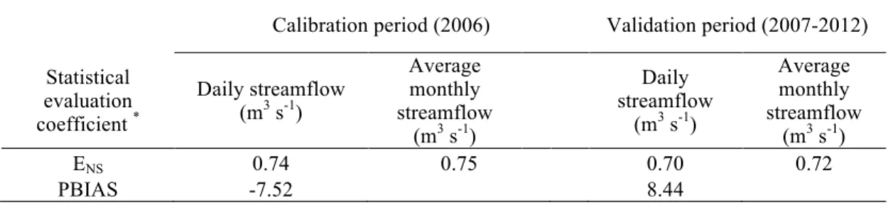
Table 2. Statistical evaluation for AgES-W simulated daily and average monthly Upper CCW streamflow. Calibration period (2006) Validation period (2007-2012) Statistical evaluation coefficient * Daily streamflow (m3 s-1) Average monthly streamflow (m3 s-1) Daily streamflow (m3 s-1) Average monthly streamflow (m3 s-1) ENS 0.74 0.75 0.70 0.72 PBIAS -7.52 8.44 * Note: E
NS = Nash-Sutcliffe efficiency; PBIAS = bias or relative error (%).
Table 2 shows that all statistical evaluation coefficients for daily streamflow decreased slightly for the validation period from 2007-2012. In particular, the ENS coefficient
decreased from 0.74 to 0.70 and PBIAS decreased from -7.52% to 8.44%, meaning that AgES-W switched from slight underprediction to slight overprediction for daily
streamflow. Table 2 also shows that all statistical evaluation coefficients for average monthly streamflow worsened slightly for the validation simulation period as compared to the calibration simulation period. Average monthly decreases were of similar magnitude as the decreases in daily streamflow. Average monthly observed and AgES-W simulated streamflow for the validation period from 2007-2012 are shown in Figure 4.
Figure 4. Monthly Upper Cedar Creek Watershed AgES-W simulated and observed streamflow (m3 s-1) at
gauge F34 (validation period – 1/1/2007 to 6/30/2012).
Daily observed and AgES-W simulated total N results for the 2006 calibration period are shown in Table 3. In general, the AgES-W model slightly underestimated total N on a daily time-step for the calibration as shown by the negative value for PBIAS (-9.11%) in Table 3. The ENS (0.68) value in Table 3 is considered satisfactory according to Moriasi et
al. (2007), and the PBIAS value is also acceptable since it is under 25%. Similar to
2006 calibration period show that ENS improved to 0.72. The PBIAS value for average
monthly total N is not shown as it is essentially the same as for the daily total N.
Similar to streamflow prediction, Table 3 shows that most of the statistical evaluation coefficients for daily total N decreased slightly for the validation period from 2007-2011 as compared to the calibration simulation period. In particular the ENS coefficient decreased
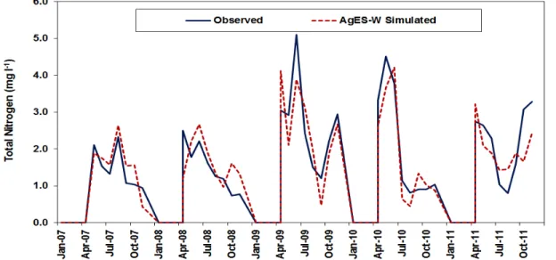
from 0.68 to 0.66; however, PBIAS improved from -9.11% to 3.63% meaning that AgES-W switched from slight underprediction to slight overprediction for daily total N (similar to calibration vs. validation for streamflow prediction). Table 3 also shows that all statistical evaluation coefficients for average monthly total N worsened slightly for the validation simulation period as compared to the calibration simulation period. Average monthly decreases were of similar magnitude as the decreases in daily total N. Average monthly observed and AgES-W simulated total N for the 2007-2012 validation period are shown in Figure 5. This figure shows that simulated average monthly total N for the validation period captured most of the observed peak total N load events quite well.
Table 3. Statistical evaluation for AgES-W simulated daily and average monthly Upper CCW total nitrogen (N) loading and daily sediment loading.
Total N – calibration period (2006)
Total N – validation period (2007-2011) Sediment load (2010-2011) Statistical evaluation coefficient * Daily total N (mg l-1) Average monthly total N (mg l-1) Daily total
N (mg l-1) Average monthly total N (mg l-1)
Daily sediment load (g l-1) ENS 0.68 0.72 0.66 0.70 0.45 PBIAS -9.11 3.63 -21.8 * Note: E
NS = Nash-Sutcliffe efficiency; PBIAS = bias or relative error (%).
Figure 5. Monthly Upper Cedar Creek Watershed AgES-W simulated and observed total N (mg l-1) at gauge F34 (validation period – 4/1/2007 to 11/9/2011).
Daily AgES-W simulated sediment loading results from April 2010 to June 2011 are also shown in Table 3. Although streamflow was slightly overestimated for the validation period, sediment loading was underestimated. Model prediction of sediment loading
should be highly correlated to surface runoff prediction. Observed surface runoff data for individual Upper CCW HRUs were unavailable; however, AgES-W underestimated streamflow for the April 2010 to June 2011 sediment loading simulation period by approximately 17% (data not shown). Table 3 shows that the daily sediment ENS and
PBIAS for the simulation period were 0.45 and -21.8%, respectively.
4. Discussion
The range of relative error (e.g., PBIAS) and ENS values for uncalibrated predictions in
this study (e.g., monthly streamflow, monthly total N, daily sediment) are within the range of others reported in the literature for various watershed models. For SWAT monthly streamflow predictions, Tolson and Shoemaker (2007) reported ENS values ranging from
0.43 to 0.86 for different gauge stations in the Cannonsville Reservoir in upstate New York. Sarangi et al. (2007) used AnnAGNPS to predict runoff and sediment losses from forested and agricultural watersheds on the island of St. Lucia in the Caribbean and reported errors of 7% to 36% for annual streamflow prediction. Kirsch et al. (2002) reported uncalibrated sediment loading results for a single year ranging from
underestimation of -50% to overestimation of 29% for eight USGS gauges in the Rock River Basin, Wisconsin, USA.
Many different factors impact the simulation of streamflow and N/sediment loading on the Upper CCW. Because the model time step is daily, it is difficult to accurately capture sub-daily (i.e., individual storms) and even daily results because of potential time shifts in the precipitation and flow data. The addition of a more physically based infiltration component, such as the Green-Ampt infiltration model used by SWAT and other
agroecosystem models, might help in this regard. Additionally, subsurface tile drains are present on the Upper CCW and may significantly impact water yield, streamflow, and N loading. Simulations were performed without the explicit inclusion of a tile drainage component, the addition of which should improve streamflow and N loading prediction accuracy. The availability of accurate climate data also plays an important role in model performance and accuracy. The effects of spatial and temporal variability in rainfall on model output uncertainty has been previously documented (e.g., Chaubey et al. 1999), and spatial variability of precipitation data represents one of the major limitations in large-scale hydrologic modeling.
The HRUs in the AgES-W simulations accessed data from only two weather stations in the Upper CCW, the BLG experimental site and the NOAA Waterloo weather station; therefore, it is possible that the distribution of rainfall over the entire watershed may be inaccurately represented. The streamflow and N/sediment loading simulation results for AgES-W almost certainly would improve if additional stream gauge and weather data were used. Ascough et al. (2012) noted that the Penman-Monteith equation used in AgES-W to estimate ET requires significant data, including, but not limited to, solar radiation, wind speed, soil characteristics, and canopy cover characteristics. Not all of this data were readily available; therefore, other required meteorological data were obtained by using the CLIGEN weather generator. Considerable uncertainty exists in weather generation, and this uncertainly is propagated in the final ET values calculated by AgES-W. Furthermore, a lack of available measured ET data for the study period makes it difficult to validate
simulated ET results. Underestimation or overestimation of ET could thereby affect the overall water and N balances, particularly during the summer months when ET demand is higher. Finally, while the distribution (i.e., the approximate percentage) of each cropping system rotation was generally known, the exact location of the various cropping systems
was not. Additional efforts are underway to provide better assessment of cropping system location.
5. Ongoing AgES-W Application to the South Fork Watershed, Iowa USA
The South Fork of the Iowa River Watershed (SFW) covers approximately 788 km2
(194,720 ac) and is dominated by pothole depressions and artificial subsurface tile
drainage needed to drain these historic wetlands. Hydric soils cover 54% of the watershed (Tomer et al. 2008a). More than 80% of the watershed is cropland. The rest of the
watershed is primarily pasture or forest with very limited urban areas. Corn and soybean are the predominant crops grown annually on 85% of the SFW area. Hydric soils occupy over 50% of the SFW making soil wetness a major concern for land management and agricultural production. To solve this problem, most fields in the SFW contain subsurface (tile) drains that flow to a network of ditches and subsequently natural stream channels. SFW monitoring results (Tomer et al. 2008a) show significant quantities of NO3-N, total P,
and sediment in streams throughout the watershed.
SFW research activities conducted by the USDA-ARS National Laboratory for
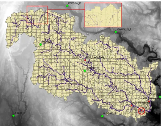
Agriculture and the Environment (NLAE) have focused on developing a water quality and land-use database to support watershed modeling and evaluation of new conservation practices. In collaboration with the NLAE, the AgES-W model is currently being used to quantify and assess spatially targeted agricultural conservation effects on water quantity and quality. Initial AgES-W input files have been developed and boundary, HRUs, and flow routing/stream channel networks delineated for the SFW (Figure 7).
In addition, preliminary baseline AgES-W simulations have been performed to assess watershed conditions in the absence of conservation practices. Comparison of baseline controls with treatment watersheds will be performed at various time steps to evaluate cumulative long-term effects of adoption of conservation practices. Conservation practice scenarios will also be performed for control watersheds as time permits. Best management practices (BMP) effects that are currently addressed in SWAT (and other models) will then be incorporated into OMS, including those that have been previously identified by the SWAT development team for improvement. A spatial inventory of current conservation practices in the South Fork includes conservation tillage practices (CP) observed at planting, conservation crop rotations, conservation reserve areas (CRP, including riparian buffers), wetland restorations, grass waterways, filter strips, manure management plans, terraces, and sediment control structures (Tomer et al. 2008b). Important BMPs for this region include tile drainage; no-tillage and residue cover; N, P, and pesticide management; and different cover crops and perennial rotations. Other BMPs have been developed
recently for reducing N in tile flow that contributes to stream flow: 1) the late spring nitrate test (LSNT, an N management tool) to guide spring side-dress application of N fertilizer (Jaynes et al. 2004); and 2) reducing tile flow and promoting denitrification of excess leached N in perched groundwater by raising tile flow gates during late fall and winter. The presence of buffers and wetlands (Tomer et al. 2003) also need to be accurately reflected in the AgES-W model.
Figure 7. AgES-W model HRU delineation for the SFW.
Final AgES-W model evaluations will include statistical comparisons of AgES-W simulated flows and N concentrations/ loads with monitoring data from the SFW outlet. Spatially distributed internal states of N and soil water in AgES-W also will be compared with field data where available and simulation results will be used to address “what if” scenarios for spatially targeted conservation in Iowa, USA. This should extend impact of field experiments by the NLAE regionally, plus allow us to simulate spatially distributed conservation practices beyond what is feasible to measure.
6. Summary and Conclusions
AgES-W reproduced (for both calibration and validation periods) the general patterns of daily and monthly hydrological and N dynamics for the Upper CCW. Model
enhancement (e.g., the addition of Green-Ampt infiltration and improved
groundwater/water table tracking components) should provide a solid foundation on which to improve AgES-W for water quantity and quality prediction at the watershed scale. Also, the topological routing scheme employed by AgES-W (thus allowing the simulation of lateral processes important for the modeling of runoff and chemical concentration dynamics) is potentially more robust than the quasi-distributed routing schemes used by other watershed-scale natural resource models such as SWAT. With a fully distributed routing concept, higher spatial resolution in combination with the lateral transfer of water and chemicals between HRUs and stream channel reaches will hopefully result in
improved H/WQ modeling for mixed-use watersheds such as the Upper CCW. The development and application of AgES-W is a significant step toward demonstrating the OMS3 framework as a viable tool for the development and maintenance of environmental models. AgES-W in OMS brings together the best qualities of a range of simulation model components under one flexible framework that allows a new generation of modeling
applications, including distributed modeling and scaling applications. From the natural resources modeling viewpoint, environmental modeling frameworks such as OMS3 have the potential to: (1) enable easier long-term maintenance and updating of model code (the complex and convoluted code structures for most current natural resource models do not facilitate maintainability); (2) reduce duplication of work by modelers for developing common basic components, as has previously occurred with considerable duplication of code in other watershed model development efforts (e.g., SWAT, AnnAGNPS, etc.); and (3) lead to better standardization of science components over time.
For the SFW, we anticipate that the spatially distributed AgES-W model can account for transport of water, sediment, chemicals from HRUs to stream channels, and with improvement in model components for spatially-targeted conservation systems will provide better estimates (than existing watershed modeling technology) of conservation system effects on water quantity and quality. AgES-W will be used to guide the selective spatial placement of conservation practices at the most sensitive locations in the SFW, where conservation practices will be most effective, instead of uniform spatial application. Finally, spatially distributed process simulation with hydrologic and biochemical
interaction across field to watershed scales should improve the assessment of complex interactions in space and time - such spatially explicit capabilities of AgES-W are not currently replicated by other models.
References
Ascough II, J.C., David, O., Krause, P., Heathman, G.C., Kralisch, S., Larose, M., Ahuja, L.R., and Kipka, H., 2012: Development and application of a modular watershed-scale hydrologic model using the Object Modeling System: Runoff response evaluation. Trans. ASABE, 55(1), 117-135.
Borah, D.K., and Bera, M., 2004: Watershed scale hydrologic and nonpoint source pollution models: Review of applications. Trans. ASAE, 47(3), 789-803.
Chaubey, I., Haan, C.T, Salisbury, J.M., and Grunwald, S., 1999: Quantifying model output uncertainty due to spatial variability of rainfall. J. Amer. Water Res. Assoc., 35(5), 1-10.
David, O., Ascough II, J.C., Lloyd, W., Green, T.R., Rojas, K.W., Leavesley, G.H., and Ahuja, L.R., 2013: A software engineering perspective on environmental modeling framework design: The Object Modeling System. Env. Modell. & Soft., 39(2013), 201-213.
Duan, Q., Gupta, V.K., and Sorooshian, S., 1992: Effective and efficient global optimization for conceptual rainfall-runoff models. Water Resour. Res., 28(4), 1015-1031.
Fink, M., Krause, P., Kralisch, S., Bende-Michl, U., and Flügel, W.-A., 2007: Development and Application of the Modelling System J2000-S for the EU-Water Framework directive. Adv. Geos., 11, 123-130. Gassman, P.W., Reyes, M.R., Green, C.H., and Arnold, J.G., 2007: The Soil and Water Assessment Tool:
Historical development, applications, and future research directions. Trans. ASABE, 50(4), 1211-1250. Hay, L.E., Leavesley, G.H., Clark, M.P., Markstrom, S.L., Viger, R.J., and Umemoto, M., 2006: Step wise, multiple objective calibration of a hydrologic model for a snowmelt dominated basin. J. Amer. Water
Res. Assoc., 42(4), 877-890.
Im, S., Brannan, K.M., Mostaghimi, S., and Kim, S.M., 2007: Comparison of HSPF and SWAT models performance for runoff and sediment yield prediction. J. Env. Sci. and Health, Part A, 42(11), 1561-1570.
Jaynes D.B., Dinnes, D.L., Meek, D.W., Karlen, D.L., Cambardella, C.A., and Colvin, T.S., 2004: Using the late spring nitrate test to reduce nitrate loss within a watershed. J. Environ. Qual., 33, 669-677.
Kirsch, K.J., Kirsch, A., and Arnold, J.G., 2002: Predicting sediment and phosphorus loads in the Rock River Basin using SWAT. Trans. ASAE, 45 (6), 1757-1769.
Larose, M., Heathman, G.C., Norton, D.L., and Engle, B., 2007: Hydrologic and atrazine simulation in the Cedar Creek watershed using the SWAT model. J. Env. Qual., 36, 521-531.
Moriasi, D.N., Arnold, J.G., Van Liew, M.W., Binger, R.L., Harmel, R.D., and Veith, T.L., 2007: Model evaluation guidelines for systematic quantification of accuracy in watershed simulations. Trans. ASABE, 50(3), 885-900.
Neitsch, S.L., Arnold, J.G., Kiniry, J.R., and Williams, J.R., 2011: Soil and Water Assessment Tool
theoretical documentation: Version 2009. Texas Water Resources Institute Technical Report 406. Texas A&M Univ. System, College Station.
Niraula, R., Kalin, L., Wang, R., and Srivastava, P., 2012: Determining nutrient and sediment critical source areas with SWAT model: Effect of lumped calibration. Trans. ASABE, 55(1), 147-157.
Pfennig, B., Kipka, H., Wolf, M., Fink, M., Krause, P., and Flügel, W.-A., 2009: Development of an extended routing scheme in reference to consideration of multi-dimensional flow relations between hydrological model entities. In: Proc. 18th World IMACS Congress and MODSIM09 International Congress on Modelling and Simulation, R. Anderssen, R. Braddock, and L. Newham (Eds.), Cairns, Australia, pp. 1972-1978.
Sarangi, A., Cox, C.A., Madramootoo, C.A., 2007: Evaluation of the AnnAGNPS model for prediction of runoff and sediment yields in St. Lucia watersheds. Biosystems Eng., 97(2), 241-256.
St. Joseph River Watershed Initiative (SJRWI), 2004: ARN 01-383 - Cedar Creek watershed management plan. Available at: www.sjrwi.org/documents/CCWMP-finaldraft081505.pdf.
Tolson, B.A., and Shoemaker, C.A, 2007: Cannonsville reservoir watershed SWAT2000 model development, calibration and validation. J. Hydrology, 337(1-2), 68-86.
Tomer, M.D., James, D.E., and Isenhart. T.M., 2003: Optimizing the placement of riparian practices in a watershed using terrain analysis. J. Soil Water Conserv. 58(4), 198-206.
Tomer, M.D., Moorman, T.B., and Rossi, C.G., 2008a: Assessment of the Iowa River’s South Fork watershed: 1. Water quality. J. Soil Water Conserv. 63(6):360-370.
Tomer, M.D., Moorman, T.B., James, D.E., Haddish, G., and Rossi, C.G., 2008b: Assessment of the Iowa River’s South Fork watershed: 2. Conservation practices. J. Soil Water Conserv. 63(6):371-379.
USDA-NASS, NASS homepage, 2001: USDA National Agricultural Statistics Service, Washington, D.C.
Available at: www.nass.usda.gov/index.asp.
USDA-NRCS, STATSGO2 homepage, 2012: Available at: http://soils.usda.gov/survey/geography/statsgo. USEPA, 2002: 2000 National Water Quality Inventory. Washington, D.C.: U. S. Environmental Protection
Agency, Assessment and Watershed Protection Division. Available at: http://water.epa.gov/lawsregs/guidance/cwa/305b/2000report_index.cfm.
Williams, J.R., 1995: Chapter 25. The EPIC Model. p. 909-1000. In: Computer Models of Watershed Hydrology. Water Resources Publications. Highlands Ranch, CO.