Exhaust emissions and environmental classifications of cars : what indicators are relevant according to external cost calculations?

Lena Nerhagen

Sara Janhäll

Exhaust emissions and environmental

classification of cars

What indicators are relevant according to

external cost calculations?

VTI notat 3A-2015

|

Exhaust emissions and envir

onmental classification of cars

www.vti.se/publications

VTI notat 3A-2015

VTI notat 3A-2015

Exhaust emissions and environmental

classification of cars

What indicators are relevant according to external

cost calculations?

Lena Nerhagen

Sara Janhäll

Diarienummer: 2014/0068-7.4 Omslagsbild: VTI/Hejdlösa Bilder Tryck: LiU-Tryck, Linköping 2015

Preface

This study has been financed by Folksam. Folksam is a Swedish insurance company that for more than 30 years has undertaken traffic safety research with an emphasis on the study of real-world accidents. By analyzing the damage and injuries that occur, Folksam provides advice on the best vehicles and on how accidents and injuries can be prevented. Environmental aspects have also been assessed in recent years, and Folksam now produces a yearly report on “Safe and Sustainable” new cars. Currently the guidelines developed by Folksam focus on the emissions of CO2 using the criteria determined by the

EU. In this study we discuss, based on methods developed in EU-funded research projects on external cost calculations, what other aspects may be relevant to consider in order to account for the overall environmental impact of exhaust emissions from cars.

We thank Folksam, in particular Maria Krafft and Anders Kullgren, for financial support and for useful comments during the course of the work.

Borlänge, November 2014

Lena Nerhagen Project Leader

Quality review

Anna Mellin reviewed and commented on the report at a review seminar carried out on 28 May 2014. Lena Nerhagen has made alterations to the final manuscript. The research director Mattias Viklund examined and approved the report for publication on 1 December 2014. The conclusions and recommendations expressed are the authors’ and do not necessarily reflect VTI’s opinion as an authority.

Kvalitetsgranskning

Granskningsseminarium genomfört 28 maj 2014 där Anna Mellin var lektör. Lena Nerhagen har genomfört justeringar av slutligt rapportmanus. Forskningschef Mattias Viklund har därefter granskat och godkänt publikationen för publicering 1 december 2014. De slutsatser och rekommendationer som uttrycks är författarnas egna och speglar inte nödvändigtvis myndigheten VTI:s uppfattning.

Contents

Summary ... 5

Sammanfattning ... 7

1. Introduction ... 9

1.1. Purpose and background ... 9

1.2. Economics, external effects and (marginal) social cost ... 10

2. The impact pathway approach ... 12

Brief description of the approach ... 12

Nonlinearities ... 13

Latency and discounting ... 13

Uncertainties ... 14

2.2. IPA and emissions from cars – data, assumptions and results ... 14

Emissions and pollution from cars ... 14

Dispersion and exposure ... 15

Exposure-response functions ... 16

Monetary valuation ... 18

Gasoline versus diesel – findings in the literature ... 20

3. External cost of diesel versus gasoline cars in Sweden ... 22

3.1. Emissions from cars and the vehicle fleet ... 22

Dispersion, concentrations and exposure ... 24

Health impact assessment and monetary valuation ... 25

Calculation of external environmental costs – an example ... 26

3.2. Other external costs for cars in Sweden ... 27

4. Indicators for sustainable cars – discussion ... 29

Summary

Exhaust emissions and Environmental classifications of cars – What indicators are relevant according to external cost calculations?

by Lena Nerhagen and Sara Janhäll

Folksam is a Swedish insurance company that for more than 30 years has undertaken traffic safety research with an emphasis on the study of real-world accidents. Folksam provides advice on the best vehicles and on how accidents and injuries can be prevented. Environmental aspects have also been assessed in recent years, and Folksam now produces a yearly report on “Safe and Sustainable” new cars. Currently the guidelines developed by Folksam focus on the emissions of CO2 using the criteria

determined by the EU. This study is based on the questions raised by Folksam on how well the criteria currently used reflect the total environmental impact of exhaust emissions. One of the questions is whether diesel cars, being more fuel efficient, are preferable to gasoline cars given the differences in for example particle and NO2 emissions.

In this paper we give an overview of the method used to calculate the external costs related to the exhaust emissions of cars, the Impact Pathway Approach (IPA). This type of assessment has previously been used to compare the environmental performance of gasoline versus diesel cars in a report by the former Swedish national road administration (Vägverket, 2001) and in a recent paper on the taxation of cars in Belgium (Mayeres & Proost, 2013). We also provide an overview of recent research on the inputs used in these calculations. Based on information on emission tests of VW cars (Ecotraffic, 2012 a and b) and information from the Swedish Transport Administration, we illustrate how different aspects influence the outcome of these calculations regarding exhaust emissions from cars.

Regarding the specific question raised in this study about indicators for sustainable cars, we find that the indicators currently used, CO2 emissions, do not reflect the full environmental impact. Different

types of vehicle technologies result in different combinations of emissions. With the large variety of car models, and with important differences between type approval and ”real driving” emissions, we conclude that apart from CO2 emissions, vehicle technology should be accounted for in the

classification of cars. Concerning the difference between gasoline and diesel vehicles, important aspects to consider are:

 differences in emissions of particulates where particle size or number and composition may be important to consider in addition to, or maybe even rather than, mass

 the difference in the ratio between NOx and NO2, as it affects local NO2 and ozone

concentrations.

We also provide an example of how external cost calculations can be used to assess the performance of a car model in relation to differences in risk for severe outcomes of an accident. In principle, the same type of reasoning as for other health impacts applies. However, due to lack of data we have not had the possibility to explore the trade-off between smaller cars, with lower emissions but higher risk for severe outcomes of accidents, and larger cars. This is an issue left for future studies.

Sammanfattning

Avgasutsläpp och miljöklassning av bilar – Vilka indikatorer är relevanta baserat på beräkning av externa kostnader?

av Lena Nerhagen och Sara Janhäll

Folksam är ett svenskt försäkringsbolag som i över 30 år genomfört forskning om trafiksäkerhet baserat på analyser av inträffade trafikolyckor. Folksam tillhandahåller vägledning om bra produkter och om hur olyckor och skador kan förebyggas. Under senare år har Folksam även börjat arbeta med miljöfrågor och tar nu årligen fram en rapport om “Säkra och Miljövänliga” nya bilar. För närvarande baseras miljöklassningen på utsläppen av CO2 enligt de riktlinjer som tagits fram av EU. Motivet till

denna rapport är att Folksam önskar få belyst om nuvarande underlag för klassificering på ett bra sätt speglar för den totala miljöpåverkan från en viss bilmodell. En mer specifik fråga är om dieselbilar, som är mer bränsleeffektiva, är att föredra framför bensinbilar trots skillnader i utsläpp när det gäller partiklar och NO2.

I denna rapport beskriver vi översiktligt den metod som används för att beräkna de externa

kostnaderna för bilars emissioner. Denna metod har tidigare använts i en studie av Vägverket (2001) för att jämföra miljöpåverkan mellan bensin- och dieselbilar, liksom i en nyligen genomförd studie gällande beskattning av bilar i Belgien (Mayeres & Proost, 2013). Vi gör också en sammanfattning av aktuell forskning om vilka indata som bör användas i denna typ av beräkningar liksom hur denna information har använts som underlag i policy forskning. Baserat på information om utsläppstester som genomförts av Ecotraffic (2012 a och b), samt information från Trafikverket om emissions-faktorer i den svenska bilparken, illustrerar vi hur olika aspekter påverkar utfallet av denna typ av beräkningar.

När det gäller den specifika frågan om vilka indikatorer som bör användas för miljöklassning av bilar har vi funnit att nuvarande indikator, emissioner av CO2, inte avspeglar den fulla miljöpåverkan av en

viss bilmodell. Olika teknologier resulterar i olika mix av emissioner. Givet att det finns väldigt stor variation i bilmodeller, och givet att det är stor skillnad mellan emissionsfaktorer från testcykler och de i verklig körning, är vår slutsats att utöver CO2 så bör skillnader i teknologier utgöra en grund för

miljöklassning av bilar. När det gäller skillnaden mellan bensin- och dieselbilar så är följande aspekter viktiga att ta hänsyn till:

 skillnaden i emissioner av partiklar där det kanske framförallt är storlek eller antal som är viktiga markörer, snarare än massa

 skillnaden i kvoten mellan NOx och NO2 eftersom det har betydelse för lokala koncentrationer

av NO2 och ozon.

Vi har även gett ett exempel på hur beräkning av externa kostnader kan användas för att bedöma skillnaderna mellan olika bilmodeller när det gäller minskad risk för att skadas allvarligt i en olycka. Det är i princip samma resonemang som ligger till grund för denna beräkning som andra som handlar om risker för påverkan på människors hälsa. Brist på data har dock medfört att vi inte kunnat göra en jämförelse mellan mindre bilar med lägre emissioner men som kanske är mindre trafiksäkra och större bilar för vilket det omvända gäller. Den frågan kan vara intressant att undersöka i framtida studier.

1.

Introduction

1.1.

Purpose and background

Folksam is a Swedish insurance company that offers a wide variety of insurance, savings and loan products. For more than 30 years, Folksam has undertaken traffic safety research with an emphasis on the study of real-world accidents. By analyzing the damage and injuries that occur, Folksam provides advice on the best vehicles and on how accidents and injuries can be prevented. Environmental aspects have also been assessed in recent years, and Folksam now produces a yearly report on “Safe and Sustainable” new cars. Currently the sustainability guidelines developed by Folksam focus on the emissions of CO2 using the criteria determined by the EU1.

The motive for this study is a question raised by Folksam on how well the criteria currently used, which have a focus on CO2 emissions, reflect the total environmental impact of exhaust emissions.

One of the questions is whether diesel cars, being more fuel efficient, are preferable to gasoline cars given the differences in for example particle and NO2 emissions. Since the latter emissions are known

to have health impacts, if they are to be accounted for there is also the question of how to compare these health impacts of the cars with their safety aspects.

Within the EU, the work on the environment in relation to cars is to protect air quality.2 _Different

means are used to accomplish this. One way is to use emission performance standards for CO2.3

Another is the system of Euro standards establishing emission limits for other harmful pollutants such as nitrogen oxides and particulates.4 _{There is also an EU Directive in place since 2009 (2009/33/EC),}

which requires that energy and environmental impacts linked to the operation of vehicles over their whole lifetime are to be taken into account in vehicle purchase decisions of public authorities. These lifetime impacts of vehicles shall include at least energy consumption, CO2 emissions and emissions of

the regulated pollutants NOx (nitrogen oxide), NMHC (non-methane hydrocarbons) and particulate matter.

The EU also grants Member States the right to implement tax incentives intended to encourage earlier implementation of the new limits. In Sweden, new light duty vehicles (including cars) that are

classified as clean vehicles are exempt from tax for five years. In addition to having CO2 emissions

below the EU limits, the cars should also be either Euro 5, Euro 6, hybrid electric, plug-in hybrid or electric vehicles.

The purpose of this study is to investigate if there is a need to complement the current guidelines of “safe and sustainable” new cars with indicators related to other exhaust emissions than CO2. To this

end, we will use the approach of external cost calculation that is used within the EU to assess the societal impact of emissions.5_{. In this report we therefore give an overview of the method used to}

calculate the external costs related to the exhaust emissions of cars. We also provide information on the most recent information on the inputs to be used in these calculations. Moreover, we use an

1_{The following formula is used to calculate whether a car is to be exempt from tax (see}

http://www.transportstyrelsen.se/sv/Vag/Miljo/Klimat/Miljobilar1/): 0.0457 * (mass of vehicle in kilo - 1372) + (95 or 150). 95 is used for gasoline or diesel cars and 150 is used for biofuel-powered cars.

2 _{http://ec.europa.eu/enterprise/sectors/automotive/environment/co2-emissions/index_en.htm}

3 _{Regulation (EU) No 510/2011 setting emission performance standards for new light commercial vehicles as}

part of the Union's integrated approach to reduce CO₂ emissions from light-duty vehicles.

4 _{European emission standards define the acceptable limits for exhaust emissions of so called conventional}

pollutants (not CO2) of new vehicles sold in the EU. For more information see Commission Regulation (EC) No

692/2008 of 18 July 2008 implementing and amending Regulation (EC) No 715/2007 of the European

Parliament and of the Council on type-approval of motor vehicles with respect to emissions from light passenger and commercial vehicles (Euro 5 and Euro 6) and on access to vehicle repair and maintenance information.

5 _{This is the type of calculation used in the design and assessment of EU regulations such as the air quality}

example to describe how different aspects influence the outcome of such calculations. This type of assessment has previously been used to compare the environmental performance of gasoline versus diesel cars in a report by the former Swedish National Road Administration (Vägverket, 2001) and in a recent paper on the taxation of cars in Belgium (Mayeres and Proost, 2013). Our focus is on the health impact, but we will in our example also briefly discuss how the health risks of exhaust emissions can be compared with the safety performance and the climate impact of a car.

The outline of the paper is as follows. The next section in this chapter provides a brief description of the concept of external effects and how it relates to marginal social cost (or external cost) calculations. We also describe how this information, according to economic theory, is useful for policy assessments in general, and for comparison of different types of risks in particular. In Chapter 2, we describe the method of IPA in greater detail since it is used to calculate the external cost of exhaust emissions. We also provide an overview of recent research on the inputs used in these calculations and how the method has been used in recent policy research. In Chapter 3, based on information on emission tests of VW cars (Ecotraffic, 2012 a, b) and information from the Swedish Transport Administration, we illustrate how different aspects influence the outcome of these calculations regarding exhaust

emissions from cars. We also briefly discuss the implications of accounting for safety aspects and for

CO2 emissions. The paper ends with a discussion on the use of indicators in Chapter 4.

1.2.

Economics, external effects and (marginal) social cost

The main question raised by Folksam is whether the outcome of the focus on CO2 in the assessment of

new cars may result in negative environmental impacts in other ways that should be accounted for in their assessment. This is one example of how decisions to improve societal welfare can imply the need to make trade-offs between different objectives. In some cases these choices are straightforward with few and clearly defined costs and benefits. However, this is most often not the case. Therefore, in economics, economic valuation methods have been developed with the purpose of “placing a price” on different types of impacts in order to make them comparable. The basis for “placing a price” is the impact of an activity on third parties6 _{(measured as marginal social costs); the term external cost is}

commonly used in economics.

There are two main reasons for obtaining this information. One is that if we have an estimate of the external cost, a so-called Pigouvian tax can be placed on the activity. As discussed in economic theory, internalizing external costs through Pigouvian taxes will correct for the market failure caused by the activity. This is because prices are a bearer of information and sends signals in a market system. Pigouvian taxes give actors (consumers and producers as well as policy makers) economic incentives to act and to change behavior since they raise the cost of shirking. However, for various reasons, a Pigouvian tax is not always possible to impose on an activity. Hence, the other reason for having information on the external cost is because it is useful for the design of other policy measures, e.g., standards and limit values (see Sterner, 2003, for a thorough discussion on the design of policy measures). In the preparation of such regulations, information on external costs can be used to compare the benefits and costs of different alternatives and different impacts.

Air pollution, which is the problem in focus in this study7_{, comes from various sources and has several}

different impacts on the natural environment and/or on human health. Moreover, the effects can occur instantly but also some time into the future. In order to compare negative impacts of pollution in decision making, the IPA has been developed in the EU-funded ExternE projects (Friedrich and Bickel, 2001; Bickel and Friedrich, 2005) and is now used in preparations of regulatory policy

6 _{Third parties are those who do not take part in a market transaction but are still influenced by it.} 7 _{This report focuses on the problems related to air pollution, but the underlying theory and the methods}

described are the same as those used to calculate the external cost of noise; see Andersson and Ögren (2007) for a Swedish example. Air pollution also has a negative influence on the natural environment but in this report we only focus on the calculation of external health costs.

proposals at the EU level. In this method, the external cost calculation is based on an assessment of the impacts of the emissions on the environment and/or human health and the economic value placed on these impacts. The US Environmental Protection Agency (EPA) has developed a similar tool referred to as BenMAP8_.

Early examples of these types of calculations for the transport sector are found in Small and Kazimi (1995) and Delucchi (2000), who referred to them as the damage cost approach. In the environmental economics literature it has instead been called the dose-response method and can be applied to different types of pollution. This approach is also used to obtain external cost estimates of accident risk (see, e.g., Fridstrom, 2011). To do this there is a need to quantify the effect of a policy change in terms of reduction in accident risk and the expected change in injuries or fatalities. Furthermore, a monetary value has to be placed on the injury or fatality. For the latter, the value of a statistical life (VSL) is commonly used, or the value of a life year lost (VOLY). We provide an example of how this can be done in our example in Chapter 3 using information from the Norwegian Institute of Transport Economics.

For CO2, however, there is an ongoing scientific discussion on what approach to use since the

quantification of the impacts of these emissions on society is more difficult (see Brännlund, 2009 and Idar Angelov, Hansen and Mandell, 2010). In this study we will use the value presented in an updated version of the Handbook for External Cost Calculation (Ricardo-AEA, 2014) in our example in Chapter 3.

2.

The impact pathway approach

The project ExternE (External costs of Energy) started in 1991 financed by the European Commission. Initially, its aim was to assess the externalities associated with electricity generation. By the late 1990s the methodology was adapted for accessing transportation externalities. The impact pathway approach was developed within this project (European Commission, 2003; Krewitt, 1998) and it is presented in great detail in Friedrich and Bickel (2001). The model has been used in several research projects in the EU, for example UNITE9_{. It has also been used in the revision of the previous air quality directive, the}

CAFE10 _{program, as well as the more recent air policy assessments (Holland, 2014).}

Brief description of the approach

IPA is divided into four different steps; see Figure 1. The first step is to identify the source and quantity of the emissions. The second step is to calculate the dispersion of these emissions throughout the area of interest for the study. In the third step, the exposure-response functions are used to quantify the impacts, i.e., for example the health effects of the studied emission. Finally, a monetary valuation is made using world market prices if possible. However, since human health does not have a world market price, other methods are used, such as stated or revealed preferences studies (Hurley et al., 2005). The impact pathway approach can indicate the relevance of different emissions in comparison with each other as well as provide an estimate of the total impact of traffic emissions.

Figure 1 The principal steps of the impact pathway approach (Source: Bickel and Friedrich, 2005) A more formal description of how the external health cost calculations are done in IPA is given by equation (1), where the first and second steps in Figure 1 are the basis for the first input, i.e.,

9 _{Unification of Marginal Costs and Transport Accounts for Transport Efficiency (UNITE), project funded by}

the European Commission.

10 _{The Clean Air for Europe (CAFE) programme, was put forward by the Commission in 2001. Its key objective}

was to bring all existing air quality legislation into a new single legal instrument. The programme resulted in the current Ambient Air Quality Directive (2008/50/EC).

exposure11_{. It describes the yearly cost (benefit) due to an increase (reduction) in concentration, C,}

from a change in emissions of a certain pollutant from a specific source: External health cost = ∆yearly exposure ∙ effect ∙ value =

= (∆Ca;i ∙ POP) ∙ (Ba;j ∙ Pi;j) ∙ Vj (1)

where

∆Ca;i = change in average annual exposure for pollutant i (µg/m3)

POP = population exposed to ∆Ca;i

Ba;j = baseline annual health impact rate in population for health impact j (number of cases

per inhabitant)

Pi;j = effect on health impact j per µg/m3 of pollutant i (relative risk)

Vj = value of health impact j.

This calculation has to be done separately for each pollutant since the effect estimates Pi;j (the

exposure-response functions) are likely to differ. The cost calculated for each pollutant and each health endpoint can then be added up to arrive at the total yearly health cost for the change in emissions from each source, such as a car.

What this expression reveals is that this calculation requires data from several different sources. What is done in one step will also influence the information needed and assumptions made in subsequent steps. In theory this calculation is quite straightforward, yet in practice it is more problematic since it is difficult to determine with certainty what the health impacts of a certain pollutant are. Hence, when choosing what pollutants and health endpoints to include in the calculation, the analyst has to consider how to include all different health endpoints while avoiding double counting. In the following we give a brief overview of some important issues discussed in the literature regarding these kinds of

calculations (see Mellin and Nerhagen, 2010, for more details).

Nonlinearities

The calculation presented in equation 1 rests on an assumption of linear relationships and in most applications linear relations are assumed (Small and Kazimi, 1995; Olsthoorn et al., 1999; Bickel et al., 2006; Jensen et al., 2008). Why this is a reasonable assumption for most part of the chain is discussed at length in Small and Kazimi (1995) and Bickel et al. (2006).However, assuming linearity implies that only minor changes from the current state can be evaluated. The reason for this is that both economic values and exposure-response relationships are likely to change the further we move away from the current situation.

Latency and discounting

Another aspect to account for in these calculations is that the health effects caused by air pollution can occur instantly but also some time into the future, i.e., with latency. Hence, when calculating the external cost for a certain health impact, there needs to be correspondence between the estimated health impact and the economic value used. For chronic diseases such as chronic bronchitis, the value used should reflect that this disease will affect an individual’s quality of life several years into the future. In economics, this is accounted for by discounting the monetary value placed on a loss in quality of life.

Uncertainties

These types of calculations are complex and based on assumptions in every part of the chain. Hence, for the user of the result it is important to be able to assess the reliability of the results and how they are influenced by the assumptions made. One way to validate the results is to compare them with similar calculations where other models have been used. For this reason, transparency has been one of the objectives in the ExternE project (Friedrich and Bickel, 2001).

2.2.

IPA and emissions from cars – data, assumptions and results

Friedrich and Bickel (2001) give a thorough description of the method and the relevant input data for transport that was used in the EU project UNITE. However, understanding environmental and health impacts is complicated and new scientific evidence needs to be accounted for, which requires

continuous updates. In 2005, Bickel and Friedrich provided an updated version that was used in other EU-funded research projects such as HEATCO and CAFE12 _{and as a basis for a handbook on external}

cost calculations for transports (Maibach et al., 2007).

Following the current revision of the EU Thematic Strategy on Air Quality13_{, WHO has coordinated}

two projects, REVIHAAP (Review of Evidence on Health Aspects of Air Pollution) and HRAPIE (Health Risks of Air Pollution in Europe), to provide the latest scientific evidence on the health effects of all pollutants regulated in current directives.14 _{An impact assessment and a cost-benefit analysis}

(CBA) that to some extent use these updated exposure-response relationships have also been carried out. The monetary values used in the CBA are updated from the values used in the analysis for the CAFE program (Holland, 2014).

In the following we briefly present data and assumptions underlying these calculations. We also present some results from recent calculations of relevance for the purpose of this study.

Emissions and pollution from cars

Outdoor air pollution is a mixture of multiple pollutants originating from a myriad of natural and anthropogenic sources. Traffic is the most important source of outdoor air pollution in urban areas in Sweden (Swedish EPA, 2010). Like other combustion, engines contribute to possibly harmful substances such as particulate matter (PM), nitrogen oxides (NOx), carbon monoxide (CO), and organic compounds (VOC). An additional source in Swedish urban areas is the contribution of particulate matter from road wear. While the latter are mainly coarse particles that are large in size (PM10-2.5), exhaust-related emissions are small in size (PM2.5) but large in numbers.

The main difference between a traditional gasoline and a diesel engine is that diesel engines have relatively high fuel efficiency but create more health threatening exhaust emissions, e.g., PM and NOx. Gasoline cars on the other hand emit more organic compounds (VOC) than diesel cars. In addition, technological improvements such as diesel particle filters have reduced some of the

emissions but not others, while catalysts reduce NO emissions at the expense of increased emission of NO2 and NH3.

The reason for the reductions in emissions over time is new emission standards for vehicles. From 2011, new cars have to comply with the standard Euro 5 with limit values as presented in Table 1. Yet another standard, Euro 6, will be in place from 2015. Euro 6 implies additional requirements on diesel vehicles, especially for nitrogen oxides. Hence, additional reductions in some emissions are to be expected.

12 _{Unification of Marginal Costs and Transport Accounts for Transport Efficiency (UNITE). Harmonised}

European Approaches for Transport Costing (HEATCO). Clean Air For Europe (CAFE).

13 _{http://ec.europa.eu/environment/air/review_air_policy.htm}

14

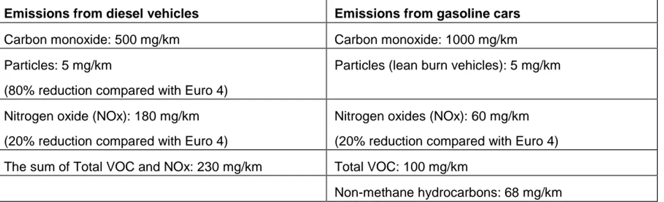
Table 1 EURO 5 limit values (source: Europa.eu, 2014)

Emissions from diesel vehicles Emissions from gasoline cars

Carbon monoxide: 500 mg/km Carbon monoxide: 1000 mg/km Particles: 5 mg/km

(80% reduction compared with Euro 4)

Particles (lean burn vehicles): 5 mg/km

Nitrogen oxide (NOx): 180 mg/km (20% reduction compared with Euro 4)

Nitrogen oxides (NOx): 60 mg/km (20% reduction compared with Euro 4) The sum of Total VOC and NOx: 230 mg/km Total VOC: 100 mg/km

Non-methane hydrocarbons: 68 mg/km However, when performing calculation for new cars the problem is that emission factors in real driving conditions differ from the type-approval values presented by the manufacturer since the latter are based on a standardized test cycle (called NEDC). The discrepancies between type-approval and real-world fuel consumption and CO2values are discussed in a recent working paper from ICCT

(International Council on Clean Transportation). The paper presents results from an assessment of 2001-2011 European passenger cars (Mock et al., 2012).

According to their results, there is a gap between type-approval and real-world fuel consumption/CO2

values, which increased from about 8% in 2001 to 21% today. Reasons for this are 1) that he experimental design allows for differences in the protocol presently used by many developers to minimize the CO2emissions within the standard, 2) an inability of the current test cycle to represent

all the different real-world driving conditions that exist, and 3) an increasing share of vehicles equipped with air conditioning systems. A recent Norwegian study confirms that there is a difference between type-approval and real-world values also for other pollutants, and also for new cars,

complying with the Euro 6 standard, a difference remains (Hagman and Amundsen, 2013). One explanation for this seems to be cold starts.

An additional aspect to account for in these calculations is that the emissions from a car also take part in chemical reactions. Ozone is a secondary pollutant and the concentration depend on sunshine, NO, NO2, and organic species. In city centers, where traffic emissions are normally high, NO emissions

rapidly reduce the ozone concentrations by reacting with ozone to form NO2. However, if ozone is

absent NO will not form NO2 as fast. Thus, it is of increasing importance to know the part of NOx

emission that is emitted as NO2, and to not use NOx and NO2 interchangeably. In addition, the effect

of emissions on the ozone concentration depends on available sunshine and if the ozone formation is NOx or VOC limited. Thus, the effect of increasing NOx emissions in VOC limited areas is not closely related to ozone formation and should not bear that cost. A recent example of this type of modeling for Swedish conditions is Fridell et al. (2014). They perform modeling for the Västra Götaland Region and discuss how composition of emissions can influence the outcome of these calculations as well as differences between regions.

NOx, as well as some other emissions, also contribute to the formation of secondary aerosols (for example nitrates), which also needs to be accounted for in the external cost calculation. This formation is also affected by climate and is thus likely to differ between different parts of Europe even though there is a limited understanding of secondary aerosol formation processes (Hallquist et al., 2009).

Dispersion and exposure

In order to perform these calculations, the population exposure to the different pollutants has to be assessed. Dispersion models combined with population data are used to this end. Since the pollutants have very different chemical and physical properties, the relation between emission and exposure differs substantially between pollutants. Thus, nonlinear relationships in the exposure calculation need

to be accounted for in the calculations (Muller and Mendelsohn, 2007; Jensen et al., 2008). One such relationship is that population exposure will vary depending on the location of the emission source. Hence the cost for a pollutant that increases concentrations locally will be higher if it is released in urban areas where the population density is high. Nonlinearity can also occur since the formation of secondary pollutants (resulting from chemical transformations) depends on what pollutants are already in the air or on the amount of the pollutant released. Small and Kazimi (1995) argue that for small changes in emissions, these relationships can be assumed to be linear while other studies have shown mixed results (Muller and Mendelsohn, 2007; Jensen et al., 2008, Janhäll et al., 2013).

Regarding emissions that are deposited close to their source, there is a question of what concentrations levels to use in the exposure assessment since they are generally high close to the source but then diminish rather quickly. In urban areas in Sweden for example, the relationship between smaller exhaust-related PM and the total measured concentration (PM2.5/PM10) varies depending on where the

measurement is taken. In a city street in central Stockholm, Sweden, the ratio is only 0.3, and at a city center rooftop 0.415_{. The reason is that coarser PM is deposited closer to the source. Studies of health}

impacts have used measurement values from fixed monitoring stations in the urban background (e.g., rooftops) and therefore values corresponding to such locations should be the basis for the extrapolation (Ostro, 2004).

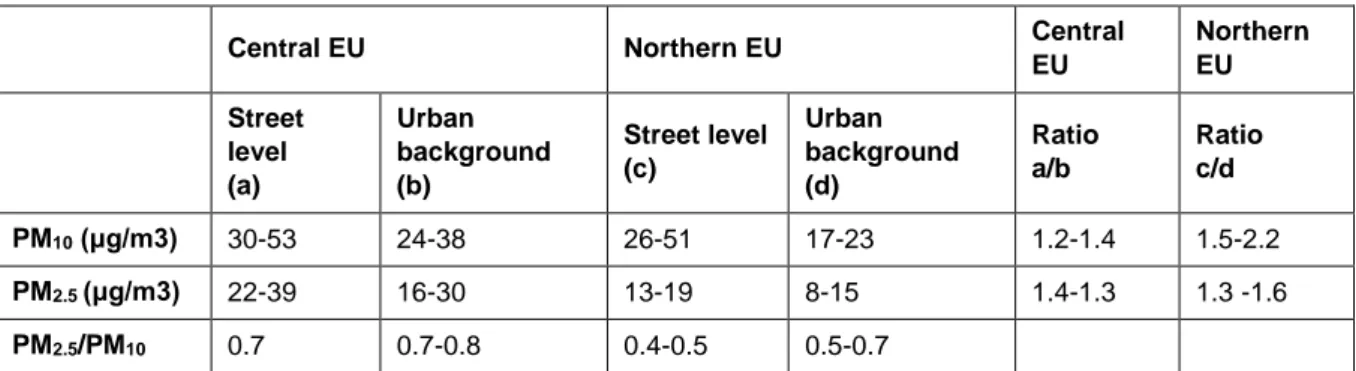
When making comparisons between estimates of health outcomes and the relationship between emissions and exposure, it is important to understand that there are significant differences in for example PM size and content between different parts of Europe. Table 2 presents a summary of some estimates of PM2.5 and PM10 in different parts of Europe. The ratio PM2.5/PM10 is 0.75 in central

Europe while it is 0.5 in the northern parts. Forsberg et al. (2005) give the same pattern for Sweden but also report lower concentrations of PM10 in northern Sweden, which is due to lower concentrations of

secondary PM originating from the European mainland.

Table 2 Illustration of variation in PM concentrations within the EU (source: own calculation based on results from CAFE WGPM, 2004, Table 6.2)

Central EU Northern EU Central

EU Northern EU Street level (a) Urban background (b) Street level (c) Urban background (d) Ratio a/b Ratio c/d PM10 (μg/m3) 30-53 24-38 26-51 17-23 1.2-1.4 1.5-2.2 PM2.5 (μg/m3) 22-39 16-30 13-19 8-15 1.4-1.3 1.3 -1.6 PM2.5/PM10 0.7 0.7-0.8 0.4-0.5 0.5-0.7

Exposure-response functions

Exposure-response functions are mainly obtained from epidemiological studies. In these studies, the aim is to define the human health impact of different substances based on, e.g., statistical analyses and measurements. One example of a common method in epidemiology is to use time series data. The researcher looks for the correlations between a daily concentration of a (mix of) pollutant(s) that a population is exposed to and, e.g., the number of hospital admissions for asthma attacks (Bickel and Friedrich, 2005).

In general, the scientific research strongly indicates that traffic emissions do generate a negative impact on human health (Sehlstedt et al., 2007; American Heart Association, 2010). External cost

15 _{Information obtained from http://www.slb.nu and measurements at Hornsgatan (street level) and Torkel}

calculation focuses on the health impact of each specific source pollutant since this information is needed in order to address the problem at the source. However, in epidemiological studies it is difficult to separate the contribution from individual pollutants (Sehlstedt et al., 2007; American Heart

Association, 2010). One complication is that many emissions are correlated and hence it may be difficult to state exactly which pollutant causes which effect. Epidemiologic studies are often based on measurement data and measurements are only done for a few pollutants. Therefore NOx is often used

as an indicator for other pollutants from traffic since there are long measurement series for NOx.

However, as discussed in, e.g., Johansson et al. (2013), the ratio between NOx and exhaust PM is

different today than a number of years back and therefore exposure-response functions based on NOx

do not reflect the health impact of exhaust PM emissions today.

Recent evidence suggests that emission PM is considered to be the main source for external health costs. The effects of PM on human health depend heavily on size and content. The size decides where in the breathing system the PM will deposit, as well as the probability that it will deposit at all or just follow the air out again. PM larger than 10 µm mainly gets stuck on the nose hairs etc. and do not enter the breathing system to a significant extent. This is why only PM smaller than 10 µm are included in the regulations, i.e., PM1016. PM smaller than 2.5 µm (PM2.5) generally passes down

through the throat. Even smaller PM, in the range of 0.05 µm, can penetrate all the way into the alveolar region and the smallest can even pass directly into the blood system following the gas

molecules. The possibility of breathing the PM out again is highest in the size range 0.3 µm. Thus, the particle size is probably of largest importance for the toxicity of PM.

The content of the PM deposited in different parts of the breathing system is also important, as, e.g., soot PM from exhaust may have larger toxicity than similar sized PM of other content. A lot of effort is being put into understanding the toxicity of different PM and evaluating the health effect related to different sources.

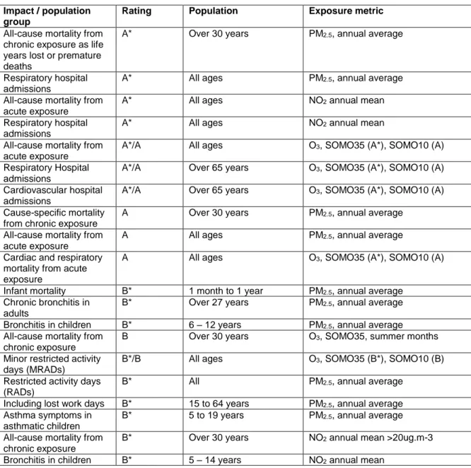
Based on the results from the recent WHO projects REVIHAAP and HRAPIE, a number of exposure-response functions have been suggested for use in external cost calculations; see Table 3 (WHO 2013a). The functions are classified using a system where those for which confidence is highest are given an “A” rating, and those for which confidence is lower are assigned a “B”. Furthermore, an asterisk “*” is added to the rating for effects that are additive. They are in some cases different from those used in the analysis for the CAFE program. However, in the CBA undertaken by Holland (2014), not all of the functions recommended in HRAPIE were used. The reason for this was lack of exposure date and the risk of double counting in the case of ozone and NO2 regarding chronic

mortality. Hence, there are several health outcomes related to air pollution but not all are relevant to consider when undertaking an IPA. Furthermore, some may not be possible to include due to lack of data.

16 _PM

Table 3 List of health impacts – HRAPIE (Source: Holland, 2014)

Impact / population group

Rating Population Exposure metric

All-cause mortality from chronic exposure as life years lost or premature deaths

A* Over 30 years PM2.5, annual average

Respiratory hospital admissions

A* All ages PM2.5, annual average

All-cause mortality from acute exposure

A* All ages NO2 annual mean

Respiratory hospital admissions

A* All ages NO2 annual mean

All-cause mortality from acute exposure

A*/A All ages O3, SOMO35 (A*), SOMO10 (A)

Respiratory Hospital admissions

A*/A Over 65 years O3, SOMO35 (A*), SOMO10 (A)

Cardiovascular hospital admissions

A*/A Over 65 years O3, SOMO35 (A*), SOMO10 (A)

Cause-specific mortality from chronic exposure

A Over 30 years PM2.5, annual average

All-cause mortality from acute exposure

A All ages PM2.5, annual average

Cardiac and respiratory mortality from acute exposure

A All ages O3, SOMO35 (A*), SOMO10 (A)

Infant mortality B* 1 month to 1 year PM2.5, annual average

Chronic bronchitis in adults

B* Over 27 years PM2.5, annual average

Bronchitis in children B* 6 – 12 years PM2.5, annual average

All-cause mortality from chronic exposure

B Over 30 years O3, SOMO35, summer months

Minor restricted activity days (MRADs)

B*/B All ages O3, SOMO35 (B*), SOMO10 (B)

Restricted activity days (RADs)

B* All PM2.5, annual average

Including lost work days B* 15 to 64 years PM2.5, annual average

Asthma symptoms in asthmatic children

B* 5 to 19 years PM2.5, annual average

All-cause mortality from chronic exposure

B* Over 30 years NO2 annual mean >20ug.m-3

Bronchitis in children B* 5 – 14 years NO2 annual mean

In the HRAPIE report (WHO, 2013a), there is also a discussion on the recent evidence of

carcinogenicity of particulates. Specific recommendations for lung cancer incidence were not made but the proposed recommendations for all-cause and cause-specific mortality are thought to partially cover this outcome. However, as they relate only to lung cancer mortality, it is concluded that this may lead to a small underestimation of the effects.

Monetary valuation

An extensive literature deals with questions related to economic valuation in general, but also to the valuation of health risk reductions in particular. Initially, the monetary value used in the latter context was related to the financial costs lost or paid due to a health outcome. In the case of premature mortality, the present value of lost income i.e. the human capital approach, was used. Similarly, the valuation of morbidity endpoints was based on the cost of illness approach where the benefits were assumed to be equal to the savings from medical expenditure plus forgone opportunity cost for being ill. However, both of these approaches underestimate the welfare loss of a health risk reduction since they do not account for the disutility that individuals experience if the outcome occurs. Hence, current

valuation methods seek to estimate individuals’ WTP for risk reductions. These methods rest on the assumption that an individual’s WTP is an approximation of a change in utility that the risk reduction entails.17 _{A brief formal treatment of the difference between the production function approaches}

described above and the WTP approach is given in Viscusi and Gayer (2005).18

The first attempts to obtain WTP estimates relied on the use of market data using revealed preference methods. These methods derive economic values from individuals’ choice behavior in real markets. An early example in the case of mortality risk reductions was the hedonic wage model. In this case the estimate rests on the compensating wage differential that workers receive for riskier jobs. However, a major drawback with revealed preference methods is that there are a limited number of risk contexts that can be explored using actual choices. Therefore, so-called stated preference methods are increasingly used. In stated preference methods, information is obtained from survey data exploring individuals’ choice behavior. The analyst designs a choice context that resembles a market situation or a referendum. The main objection raised against stated preference methods is that it is difficult to validate that answers to these questions represent actual choice behavior (a problem often referred to as hypothetical bias).

One problem in finding economic values for this type of assessment is that few valuation studies have been designed for the type of health impacts that are relevant in the air pollution context. Hence, in addition to the uncertainties related to the economic values themselves, there are uncertainties related to the transfer of one value from one context to another. Economists refer to this as benefit transfer and as discussed by Viscusi and Gayer (2005), this type of extrapolation to other groups or contexts is based on strong assumptions.

The estimates used in the CBA by Holland (2014) are presented in Table 4. The monetary values are in most cases updated estimates of those used in CAFE. One difference compared with the monetary values used in CAFE is that estimates for the chronic mortality impact of ozone are provided as a sensitivity case. The mortality impacts are quantified both as premature mortality (VSL – value of statistical life) and the loss of life expectancy (VOLY – value of a life year). Both are reported in the results by Holland (2014) in order to be transparent about the difference in results arising from the use of these two approaches.

17 _{For more information, see the special issue of Environmental & Resource Economics (2006) 33.}

18 _{There are numerous books written on issues related to economic valuation. Overviews of economic valuation}

methods and the theory behind them are given in introductory texts in environmental economics such as Brännlund and Kriström (2012) or Tietenberg (2007). Viscusi and Gayer (2005) provide a summary of issues related to the quantification and valuation of environmental health risks in particular.

Table 4 Values for the health impact assessment in Holland, 2014 (price year 2005)

Impact / population group Unit cost Unit Ozone effects

Mortality from chronic exposure as:

Life years lost, or Premature deaths

57,700 / 133,000 1.09 / 2.22 million

€/life year lost (VOLY) €/death (VSL)

Mortality from acute exposure 57,700 / 138,700 €/life year lost (VOLY) Respiratory hospital admissions 2,220 €/hospital admission Cardiovascular hospital

admissions

2,220 €/hospital admission

Minor restricted activity days (MRADs)

42 €/day

PM2.5 effects

Mortality from chronic exposure as:

Life years lost, or Premature deaths

(all-cause and cause-specific mortality)

57,700 / 133,000 1.09 / 2.22 million

€/life year lost (VOLY) €/death (VSL)

Mortality from acute exposure 57,700 / 138,700 €/life year lost (VOLY)

Infant mortality 1.6 to 3.3 million €/case

Chronic bronchitis in adults 53,600 €/new case of chronic bronchitis

Bronchitis in children 588 €/case

Respiratory hospital admissions 2,220 €/hospital admission Cardiac hospital admissions 2,220 €/hospital admission

Restricted activity days (RADs) 92 €/day

Work loss days 130 €/day

Asthma symptoms, asthmatic children

42 €/day

NO2 effects

Mortality from chronic exposure as:

Life years lost, or Premature deaths

57,700 / 133,000 1.09 / 2.22 million

€/life year lost (VOLY) €/death (VSL)

Mortality from acute exposure 57,700 / 138,700 €/life year lost (VOLY)

Bronchitis in children 588 €/case

Respiratory hospital admissions 2,220 €/hospital admission

Gasoline versus diesel – findings in the literature

The study undertaken by Vägverket (2001) concludes that the difference between gasoline and diesel vehicles was small and that it was more important, from an environmental point of view, to choose fuel efficient cars. Ecotraffic (2002) on the other hand finds that diesel cars have higher emissions of NO x and particulates (unless they have a diesel particle filter). That diesel cars are more harmful is

also found in recent research by Mayeres and Proost (2013) and Michiels et al. (2012) based on results from external cost calculations in Belgium. According to Mayeres and Proost (2013), the external cost of diesel cars are in general higher than for gasoline cars, irrespective of Euro standard. Although emitting less CO2, the external cost is higher due to the difference in conventional pollution. This

result is modified somewhat by the findings of Michiels et al. (2012). Using a different dispersion model, they find that the outcome will depend on the amount of ozone reduction resulting from NO x

emissions. For Euro 5 cars this effect is dominant, so diesel cars outperform gasoline cars yet the same result is not found for newer cars.

However, as discussed in Lindberg (2009), regarding the results from the EU-funded research project HEATCO,it is difficult to assess how relevant the values presented in EU projects are in a Swedish context without detailed calculations (case studies). Sweden is different from continental Europe in several respects (see also discussion in relation to Table 2). Our geography is different since we have a long coast and a colder climate. Our urban areas are in most cases sparsely populated. Our car fleet has

a smaller share of diesel vehicles, although the share has increased in recent years (Kågeson, 2013), and the cars bought are often larger than the European average.

From the discussion above, one aspect that needs to be considered when comparing gasoline and diesel vehicles is the influence on ozone formation. Another important aspect in such a comparison is if there is a difference in the PM emissions. The latest CBA performed in the EU regarding air pollution policy (Holland, 2014) does not make the assumption that there is a difference in the harmfulness of these emissions between gasoline and diesel vehicles. Hence, the only reason for a difference in estimated external cost per km driven will be if there is a difference in the amount of emissions or if the cars are driven in areas with different population densities.

In the scientific literature there is an ongoing discussion on whether diesel emissions have another chemical composition and therefore are more harmful. This issue has been studied by IRAC (International Agency for Research on Cancer) and their conclusion is that diesel emissions are carcinogenic while gasoline emissions might be (Benbrahim-Talla et al., 2012). One reason for such a difference between these two technologies could be the type of PM emissions. According to Eriksson and Yagci (2009), the formation of PM is different, resulting in a difference in the sizes, composition, and number of the PM for diesel vehicles. However, current measurement of PM is focused upon mass and therefore there is a lack of health impact assessments based on particulate numbers.

3.

External cost of diesel versus gasoline cars in Sweden

In this part of the report we apply the method from the previous chapter and data from calculations done in Sweden (Nerhagen et al., 2009) to compare the environmental impacts of diesel and gasoline cars. We base the comparison on information on emissions from recent models of VW Golf. We use this type of car since it has been used in several tests and publications. It is also a good example of a common mid-sized car in Sweden.

3.1.

Emissions from cars and the vehicle fleet

The environment-related information that manufacturers present for new cars usually consists of fuel consumption and CO2emissions in addition to the Euro version and type of engine. In order to classify

a car as a clean vehicle according to the EU definition, there is also a need to know the type of fuel used and the mass of the vehicle. Table 5 summarizes some information using VW Golf as an example. As expected, the fuel consumption and CO2emissions are higher for gasoline cars, but the

levels vary between different types of cars and even between production years for the same type of car. The values presented in Table 4 are so-called “type approval values” and are average estimates calculated based on emission factors from urban and rural driving in a test cycle.

Table 5 Information presented in description of new models of VW Golf (source: VW Golf modellbroschyrer).

Volkswagen Golf

Year 2013 2013 2014 2014 2014 2014

Model 2.0 TDI 2.0 TSI 2.0 TDI 2.0 TSI GTD 2.0l GTI 2.0l

Fuel Diesel Gasoline Diesel Gasoline Diesel Gasoline

Standard Euro 5 Euro 5 Euro 5 Euro 5 Euro 5 Euro 5

Particle filter Yes No Yes No Yes No

Fuel consumption average 4.2 5.3 4.7 5.2 4.2 6

CO2 average 108 121 122 121 108 139

Curb weight 1,436 1,354 1,353 1,293 1,377 1,382

Total weight 1,970 1,880 1,860 1,780 1,850 1,850

In the following, we will illustrate how well these estimates correspond to emission factors from real driving conditions. We will also add information about PM and NOx emissions that, according to

Holland (2014), is relevant to consider when assessing the external cost of a car.

We have found information on the difference between emission factors for different types of emissions and different types of cars in tests undertaken by Ecotraffic. The relationship between different types of emissions depends on the engine and exhaust treatment technologies (Eriksson and Yagci, 2009). Table 6 summarizes the results presented by Ecotraffic (2012 a, b) from different tests on specific vehicles. As can be seen, the table reveals large differences between emission factors from the test cycle and more realistic conditions (estimates using the Artemis model). Urban driving shows higher fuel consumption and emissions for PM and NOx in addition to CO2 than the test cycle. Hence, the

results from Ecotraffic’s tests confirm the findings presented by ICCE and Hagman & Amundsen (2013). The most striking result is the difference in NOx emissions between the test results and more

Table 6 Emission factors for different types of VW diesel cars (source: Ecotraffic 2012 a, b).

Fuel consumption CO2 NOx PM Comment

l/100 km g/km g/km mg/km

Ecotraffic diesel A – model year 2010

Type approval values 4.4 (4.7) 115 (124) 0.17 0.16 Euro 5 DPF*

Artemis model urban 7.9 188 0.49 0.70 Euro 5 DPF*

Ecotraffic diesel B – model year 2010

Type approval values 4.6 (5.6) 120 (147) 0.09 0.32 Euro 5 DPF*

Artemis model urban 8.0 210 0.75 0.71 Euro 5 DPF*

Ecotraffic diesel C – model year 2011

Type approval values 4.9 (6.1) 129 (160) 0.16 0.41 Euro 5 DPF

Artemis model urban 7.7 199 0.99 1.3 Euro 5 DPF

* According to the description in the text in the report.

Table 7 displays data on emission factors from the Swedish Transport Administration’s handbook (referred to as STA in the table). The handbook shows estimates of the emission factors for the vehicle fleet for all regulated exhaust emissions (Swedish Transport Administration, 2012). These emission factors are calculated based on the average Swedish vehicle fleet and are averaged for urban and rural driving, respectively, but also for each fuel and vehicle category. Future emission factors are also provided based on scenarios of changes in vehicle technology and fleet combinations. A reduction in all future emissions can be noted, but different achievements are forecasted for different types of emissions. The emissions of diesel PM are expected to decrease by 86 % from 2011 to 2020, and the emissions of NOx by a third. The PM emission reduction for diesel is expected since many cars

currently lack diesel particle filters. The reduction in fuel consumption and thus CO2emission will not

be as large as for NOx and PM.

Table 7 Emission factors for car fleet in Sweden in 2011, 2020 and 2030 (source: Swedish Transport Administration, 2012).

Emission factors for cars

Fuel consumption CO2 NOx PM HC/THC CO

l/100 km g/km g/km mg/km g/km

STA urban gasoline

2011 9.4a _{210 0.44 1.7 1.24 5.71}

2020 8.0 a _{177 0.22 0.8 0.88 4.22}

2030 6.9 a _{150 0.18 0.6 0.74 3.86}

STA urban diesel

2011 6.9 a _{170 0.43 30.4 0.06 0.44}

2020 5.7 a _{140 0.24 4.7 0.05 0.36}

2030 4.7 a _{120 0.14 2.8 0.05 0.35}

a _{Calculated from average fuel consumption andrelation between averaged and urban CO}

The emission values used in the Swedish Transport Administration’s estimations are the results from calculations with the HBEFA model19_{, which should represent emissions from real driving conditions.}

Emission factors vary to a large degree depending on individual driving styles and factors such as meteorological conditions and number of cold starts, age of the vehicle, etc. Comparing the results in Tables 6 and 7, we find that the mean emission factor from the Swedish Transport Administration is higher than the test cycle from Ecotraffic for both diesel and gasoline, but this is not the case when compared with estimates of test cycles for real driving conditions. Hence, it is difficult to arrive at an exact estimate of emissions factors for real driving conditions.

Dispersion, concentrations and exposure

Swedish conditions result in a different composition of outdoor air pollution compared with average European urban areas. First of all, the share of diesel cars has until recently been comparatively small (Kågeson, 2010), but is now growing, increasing the emissions of NOx and exhaust PM even in areas where total traffic is steady. Due to the northern location of Sweden, meteorological differences are also important for air quality. The formation of secondary pollutants, e.g., ozone and secondary PM, differs between areas mainly due to meteorological factors. In the case of ozone, the emissions that raise the levels are NO x, CO, and VOC. The importance of abating emissions of each pollutant related

to the impact on ozone differs geographically, as some areas are more VOC limited and others more NO x limited. The ozone concentrations in Sweden are rather low in relation to the availability of

pollutants, as the access to sunshine, which is needed to form ozone, is limited.

In order to assess the impact of reduced emissions factors from new vehicles, we need an estimate of the resulting impact on the population exposure. Such an assessment requires extensive modeling, which has not been possible to perform in this project. Instead we will use results from a previous study by Nerhagen et al. (2009) to illustrate the changes that are relevant to consider in the health impact assessment. In Table 8, we have compiled the results for the emissions of exhaust PM and NOx

from light duty vehicles in Stockholm. In this study, the population in Greater Stockholm was to be 1,405,600 and the vehicle km traveled was 606 million km.

Table 8 Exposure estimates of PM and NOx from emissions in Stockholm (source: Bergström, 2008).

Estimated exposure in

Estimated exposure per ton emissions Emissions Emission factors (g/vkm) Total emissio n (ton) Greater Stockholm (person ug/m3) Other Europe (person ug/m3) Greater Stockholm (person ug/m3/ton) Other Europe (person ug/m3/ton) Exhaust PM 82 82 141,000 9,150 1,720 112 NOx 3,029 3,029 4,413,584 1,457 Nitrates 3,029 3,029 76,800 143,960 25 48

Nerhagen et al. (2009) focus on primary and secondary PM and therefore ozone formation is not included in the calculation. However, as discussed in Fridell et al. (2014), in Sweden the conditions for ozone formation differ from other parts of the world and the impact of minor changes in emissions is likely to be small. In Table 8, we have also excluded other types of secondary PM that are of minor importance and/or not directly resulting from NO x emissions. For more details about the formation of

secondary PM, see Bergström (2008). Hence, our example will reveal the most important differences between the emissions from gasoline versus diesel cars but not the complete impact20_.

19 _{http://www.hbefa.net/e/index.html}

20 _{These estimates are based on modelling total emissions and assuming that small changes in the composition of}

Health impact assessment and monetary valuation

In our study we will focus on the exposure-response functions in Table 9 since they are more certain than the others and also additive. These are of interest for the gasoline diesel comparison since PM and NOx are the emissions where the absolute and relative shares differ between fuel types. Omission of

the other health endpoints is not likely to have an important impact. According to Holland (2014), chronic mortality due to PM exposure gives rise to the highest external cost.

Table 9 Exposure-response functions used in calculation (source: Holland, 2014).

Impact / population group

Rating Population Exposure metric RR (95% CI) per 10 ug/m3

All-cause mortality from chronic exposure as life years lost or premature deaths

A* Over 30 years PM2.5, annual average 1.062 (1.040–1.083)

Respiratory hospital admissions

A* All ages PM2.5, annual average 1.0190 (0.9982–1.0402)

All-cause mortality from acute exposure

A* All ages NO2 annual mean 1.0027 (1.0016-1.0038)

Respiratory hospital admissions

A* All ages NO2 annual mean 1.0180 (1.0115–1.0245)

In order to calculate the impact of a change in concentration, we need to know the baseline risk for a certain health impact in the population. In our case we have assumed that the baseline risk is

1,000/100,000 based on the assumptions used in previous studies (Nerhagen et al., 2009; Nerhagen, Bellander and Forsberg, 2013)21_.

Table 10 Monetary values applied in calculation (source: Holland, 2014).

Impact / population group Unit cost Unit PM2.5 effects

Mortality from chronic exposure as:

Life years lost, or Premature deaths

(all-cause and cause-specific mortality)

57,700 / 133,000 1.09 / 2.22 million

€/life year lost (VOLY) €/death (VSL)

Respiratory hospital admissions 2,220 €/hospital admission

NO2 effects

Mortality from acute exposure 57,700 / 138,700 €/life year lost (VOLY) Respiratory hospital admissions 2,220 €/hospital admission

The health impact calculation gives us the number of expected additional lives saved from a reduction in the concentration of PM. For each life saved, we assume that 11.2 years are saved, based on the assumptions used in Nerhagen et al. (2009). The monetary value used is the low estimate in Table 10, i.e., 57,700 euro. The reason for using the value of a life year lost instead of the value of a statistical life is to enable comparisons with traffic accident risk. In the case of traffic accidents it is generally assumed that more years are lost per death than in health related premature deaths.

21 _{In these studies 1,010/100,000 was used for mortality and 800/100,000 for children visiting hospitals. Hence}

1,000/100,000 for the whole population seems to be a reasonable assumption. We also chose the same value so that it should have the same scaling effect in all health impact calculations. This is for the whole population, and not only for those over age 30 (the age group for which the exposure response function is derived from) since we do not have that information. According to Nerhagen et al. (2009), this will not have a small impact on the results.

Calculation of external environmental costs – an example

The aim for policy on clean vehicles, and of the advice provided by Folksam, is to reduce the external environmental cost from vehicle kilometers traveled. To illustrate how the benefit from a change in emissions from a new car can be assessed, we compare the average emissions from the current vehicle fleet in Sweden 2011 (according to the estimates by the Swedish Transport Administration) with a “hypothetical” car and its assumed emissions in real driving conditions. The emission factors for the latter is what we believe can be assumed for vehicles like a VW Golf or similar. Our assumptions are based on the information above from Ecotraffic (2012b) regarding emission factors for this brand of car. Note that the diesel vehicle is assumed to have a diesel particle filter (DPF).

Table 11 presents the values we have used in the calculation. STA urban 2011 are the emission factors for the average car in Sweden while hypothetical real emission factors are for the hypothetical cars under real driving conditions. In parentheses for the diesel car we present a higher emission factor for NO x since it appears from the tests by Ecotraffic (2012 a, b) that the emissions in real driving

conditions can be higher than modeled values for these kinds of conditions. Table 11 Emission factors used in calculation.

Fuel consumption CO2 NOx PM

Comment l/100 km g/km g/km mg/km

Gasoline

STA urban 2011 9.4 210 0.44 1.7

Hypothetical real emission factors GTI 6.9 150 0.18 0.6

Diesel

STA urban 2011 6.9 170 0.43 30.4

Hypothetical real emissions factors GTD 4.7 120 0.14 (0.99) 2.8 DPF Table 12 displays the difference in emission factors between the average vehicle and our hypothetical car, for gasoline and diesel separately and for the difference between the hypothetical gasoline and diesel car. A positive value implies a reduction in emissions, hence a benefit, while a negative value implies a cost.

Table 12 Calculated difference in emission factors between the average car in the vehicle fleet and the hypothetical cars as presented in Table 11.

FC CO2 NOx PM

l/100 km g/km g/km mg/km STA urban gasoline 2011 – Hypothetical real GTI 2.5 60 0.26 1.1 STA urban diesel 2011 – Hypothetical real GTD 2.2 50 0.29 (-0.56) 27.6 Hypothetical real emission factors GTI –GTD 2.2 30 0.04 (-0.81) -2.2 Table 13 summarizes the results from the external cost calculation. In general we see that new cars result in an improvement in all dimensions, except for NOx (depending on if we use the high or low

emission factor in Table 11). The table shows results for nitrates, which have the same emission factor as NO2 since this is a secondary pollutant that originates from the emissions of NO2. The rows shaded

grey are the results from using the higher estimate for the emission factors of NO2.

The last section of the table shows the results of the comparison between new gasoline and diesel cars (Gasoline-Diesel). According to these results, whether or not a diesel car is preferable depends on the emissions of NOx and their expected health impact as well as on the difference in PM and their

emission factor for NOx is correct, then the result is that the benefit from reductions in CO2 does not

outweigh the cost caused by the increase in the other harmful pollutants.

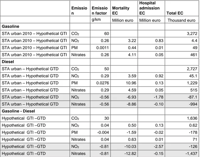
Table 13 External cost (EC) calculations based on difference in emissions in Table 12.

Emissio n Emissio n factor Mortality EC Hospital admission EC Total EC

g/km _{Million euro Million euro Thousand euro}

Gasoline

STA urban 2010 – Hypothetical GTI CO2 60 3,272

STA urban 2010 – Hypothetical GTI NO2 0.26 3.22 0.83 4.4

STA urban 2010 – Hypothetical GTI PM 0.0011 0.44 0.01 49

STA urban 2010 – Hypothetical GTI Nitrates 0.26 4.11 0.05 461

Diesel

STA urban – Hypothetical GTD CO2 50 2,727

STA urban – Hypothetical GTD NO2 0.29 3.59 0.92 45.1

STA urban – Hypothetical GTD PM 0.0276 10.96 0.13 1,229

STA urban – Hypothetical GTD Nitrates 0.29 4.59 0.05 515

STA urban – Hypothetical GTD NO2 -0.56 -6.93 -1.78 -87.1

STA urban – Hypothetical GTD Nitrates -0.56 -8.86 -0.10 -994

Gasoline - Diesel

Hypothetical GTI –GTD CO2 30 1,636

Hypothetical GTI –GTD NO2 0.04 0.50 0.13 0.62

Hypothetical GTI –GTD PM -0.004 -1.59 -0.02 -178

Hypothetical GTI –GTD Nitrates 0.04 0.63 0.01 71

Hypothetical GTI –GTD NO2 -0.81 -10.03 -2.57 -126

Hypothetical GTI –GTD Nitrates -0.81 -12.82 -0.15 -1,437

The most important findings from these calculations are:

- It is important to use emission factors from real driving conditions instead of type approval values. Especially emission factors for PM and NOx in urban areas are important for the results.

- The monetary value used for CO2 has a strong influence on the result (here 90 euro/ton).

- It is important to account for the influence of emissions in Sweden on overall air quality in Europe, here illustrated by nitrates where we have assumed they have the same impact on health as exhaust PM.

3.2.

Other external costs for cars in Sweden

In order to make a full assessment of the external cost of a car, or of an additional vehicle kilometer driven, additional aspects have to be accounted for. The handbook on external cost calculations (Ricardo-AEA, 2014) includes the following components: