A prototype system for ontology matching using polygons

A PROTOTYPE SYSTEM FOR

AUTOMATIC ONTOLOGY MATCHING

USING POLYGONS

Ana Herrero Güemes

MASTER THESIS 2006

COMPUTER ENGINEERING

A PROTOTYPE SYSTEM FOR

AUTOMATIC ONTOLOGY MATCHING

USING POLYGONS

Ana Herrero Güemes

Detta examensarbete är utfört vid Ingenjörshögskolan i Jönköping inom ämnesområdet Datateknik. Arbetet är ett led i teknologie

magisterutbildningen med inriktning informationsteknik. Författarna svarar själva för framförda åsikter, slutsatser och resultat.

Handledare: Feiyu Lin.

Examinator: Vladimir Tarasov. Omfattning: 20 poäng (D-nivå) Datum: 2006-12-15.

Abstract

When two distributed parties want to share information stored in ontologies, they have to make sure that they refer to the same concepts. This is done matching the ontologies.

This thesis will show the implementation of a method for automatic ontology matching based on the representation of polygons. The method is used to compare two ontologies and determine the degree of similarity between them. The first of the ontologies will be taken as the standard, while the other will be compared to it by analyzing the elements in both. According to the degrees of similarity obtained from the comparison of elements, a set of polygons is represented for the standard ontology and another one for the second ontology. Comparing the polygons we obtain the final result of the similarity between the ontologies.

With that result it is possible to determine if two ontologies handle information referred to the same concept.

Acknowledgements

I thank my thesis supervisor Feiyu Lin and Vladimir Tarasov, who proposed this topic, and made comments on the earlier versions of this thesis.

Sincerest thanks to my family in Spain, for their encouragement since the first moment and for being so close in spite of the distance, in the good and in the bad moments.

My gratitude to people I have met in Jönköping and friends in Spain, who have supported me every day.

Key words

Contents

1

Introduction ... 1

2

Theoretical Background ... 4

3

Implementation ... 8

3.2 EDITING THE ONTOLOGIES:PROTÉGÉ OWL ... 9

3.3 ACCESS THE ONTOLOGIES FROM JAVA:JENA... 13

3.4 COMPARING STRINGS IN ONTOLOGY MATCHING... 15

3.4.1 Previous research ... 15

3.4.2 Cases and scenarios ... 18

3.4.3 Comparison of methods... 19

3.4.4 Results... 26

3.5 FROM THE COMPARISON RESULTS TO THE POLYGONS:JMATLINK... 29

3.6 REPRESENTATION OF RESULTS:MATLAB... 31

4

Conclusion and Discussion... 37

4.1 METHOD 1:GLUE. ... 38

4.2 METHOD 2:ANCHOR-PROMPT... 39

4.3 METHOD 3:S-MATCH... 40

4.4 METHOD 4:AXIOM-BASED ONTOLOGY MATCHING... 42

4.5 METHOD 5:FCA-MERGE. ... 43

4.6 METHOD 6:MAFRA... 43

4.7 FUTURE WORK... 46

5

Results ... 48

6

References ... 49

List of Figures

FIGURE 1: STANDARD ONTOLOGY. ... 9

FIGURE 2: CLASSES IN THE STANDARD ONTOLOGY. ... 10

FIGURE 3: PROPERTIES IN THE STANDARD ONTOLOGY... 10

FIGURE 4: INDIVIDUALS IN THE STANDARD ONTOLOGY. ... 10

FIGURE 5: SECOND ONTOLOGY. ... 11

FIGURE 6: CLASSES IN THE SECOND ONTOLOGY... 11

FIGURE 7: PROPERTIES IN THE SECOND ONTOLOGY. ... 11

FIGURE 8: INDIVIDUALS IN THE SECOND ONTOLOGY... 12

FIGURE 9: SIMILARITY TABLE FOR THE COMPARISON. ... 29

FIGURE 10: SIMILARITY TABLE FOR THE COMPARISON OF SUBCLASSES. ... 30

FIGURE 11: STANDARD POLYGON... 32

FIGURE 12: SECOND POLYGON ... 33

FIGURE 13: STANDARD POLYGON FOR THE GROUP OF SUBCLASSES. 34 FIGURE 14: SECOND POLYGON FOR THE GROUP OF SUBCLASSES. ... 35

List of Abbreviations

API: Application Programming Interface.

IEEE: Institute of Electrical and Electronics Engineers. JS: Jensen and Shannon.

RDF: Resource Description Framework. OWL: Web Ontology Language.

TFIDF: Term Frequency / Inverse Document Frequency. SFS: Simplified Fellegi and Sunter.

1

Introduction

When communication between two parties is established, it has to be granted that both parties understand the information which is being exchanged in the same way. That is one of the principals of communication, and without that guarantee, a proper understanding can not be provided.

The same understanding has to be granted when two distributed ontologies are communicating. Both parties have to make sure that the concepts they are sharing are understood in the proper way.

Problems in communication can especially appear when both ontologies deal with overlapping domains of concepts. In those cases they have to relate the concepts in one of the domains to the concepts in the other one. For that purpose we use ontology matching.

This thesis aims to present and describe a new approach for matching ontologies, as well as compare it with some existing methods.

The new method proposed represents the common aspects the compared ontologies by means of polygons in order to obtain the final parameter determining the relationship between them.

1.1

Background

Ontology matching has become a key concept in the field of ontology research. Researchers all around the world have concluded that without a proper integration between ontologies, the knowledge will never be interpreted correctly, and therefore, the information will not be accurate.

Moreover, many solutions have been proposed to find correspondence between ontologies and many different applications are using those ideas, such as the AI community, the Semantic Web, Warehouses, Ontology integration, etc.

1.2

Purpose/Objectives

Despite the extensive research conducted in this field, there are still problems unsolved when dealing with ontology matching. With the aim of solving those problems and improving efficiency, a method using polygons to determine similarity between ontologies is proposed.

The algorithm for this polygon method has been developed by the Ph.D. Student in Information technology at the University of Jönköping Feiyu Lin (Feiyu Lin and Kurt Sandkuhl, 2007). The programming implementation for that algorithm and the research performed for the methods belonging to the class SecondString are the contributions of the author of this thesis.

In this thesis, the method based in polygons is described. The polygons are used to represent the main characteristics of the ontologies being compared, and by comparing the polygons, the ontologies will be compared as a result.

The purpose of the idea is giving an alternative way of matching ontologies, and solving the possible problems that the current methods have nowadays.

A new system has to be implemented in order to provide the functionality to run the new application. For this purpose a programming language has to be used as well as different programs and plug-ins.

Java is chosen as the programming language for this project due to the reason that it is the most common programming language in this field, providing a simple integration of the code into other applications.

The inputs we are going to deal with are the ontologies. Those ontologies will be implemented in OWL language. The main features of OWL will be described later in this document.

The polygons have to be represented in some mathematical way. Therefore, Matlab has been chosen as the standard program used for the mathematical requirements, given its integrating qualities.

1.3

Limitations

When we face the implementation of a system, some delimitation has to be made to clarify in which domain the project is going to be valid. Some delimitation for this project is provided in this section.

The topic of this thesis will be restricted to ontologies; no other data structure will be taken into account. The results will neither be extensible to other data integration techniques out of ontology matching.

If the input ontologies are written in other languages different from OWL, a translation should be made in order to fit the specifications of the system.

Regarding the perspective, some restrictions have to be taken into account, especially when dealing with such a large subject, where many approaches can be chosen.

The core part of the report aims at describing the implementation of the system. The sections correspond to the implementation steps followed while developing the application. That makes that the purpose of the thesis is to clarify the research tasks and justify the decisions made throughout the design and programming steps. Much technical information is also included. We can conclude that the scientific approach is the main one followed and the objective is to present the scientific community the new research done in this area.

On the other hand, the proposed system is going to be accessible for users willing to find the correspondence between two ontologies. That situation also has to be regarded in this thesis, implying the appearance of some guidance to the users as the implementation of the system is being described. The steps followed and the methodology will be constantly aimed at facilitating the role of the user when using the application.

Moreover, another important objective of this thesis is to simplify any possible further work carried out in this field and the tasks of other programmers. For that purpose, all the implementation features are explained in detail.

1.4

Thesis outline

In the introduction; the background, purpose and objectives, limitations and perspective of the project are explained. This information gives the reader a general idea about what one is going to read in the following pages, why this information is relevant, and how it is going to be presented.

In the theoretical background section, the theoretic information is provided. The core part arrives at section 3, where the implementation of the system is described. The sub-sections correspond to the tools, languages and other implementation details used, which gives an idea to the reader about the steps that were followed during the implementation of the system.

Section 4 describes the results of the project, while section 5 introduces other ontology matching methodologies and compares the results obtained with the new method and the ones corresponding to other methods in the same area of study. It also expresses some ideas for further work.

2

Theoretical Background

2.1

Ontologies

This thesis describes a new methodology for automatic ontology matching. Before arriving to that concept, it can be useful for the reader to have a general idea about what an ontology is, its main features, and the purpose of ontology designing. This section of the thesis covers all those theoretical aspects.

When defining an ontology, we have to make a reference to Gruber, (Gruber, 1993) who describes an ontology as “Specification of a conceptualization”.

As Gruber also defined (Gruber, 1992) ontology is a “Explicit formal specifications

of the terms in the domain and relations among them”.

According to Gruber (Gruber, 1992) an ontology can be described as well as “Description of the concepts and relationships that can exist for an agent or a

community of agents”.

According to the definition given by Natalya F. Noy and Deborah L. McGuinness (Noy and McGuinness, 2001) an ontology is a “Formal explicit description of

concepts in a domain of discourse”.

The definitions are many, and sometimes they contradict each other. To have a closer idea about what an ontology is, we are going to describe its functionality, its design and its components.

The sharing and reuse of knowledge among software entities is the main target of the ontology development. Ontologies give the support to implement this knowledge reuse and sharing.

Before the appearance of ontologies, other systems were in charge of the communication between knowledge producers and consumers: knowledge-based systems.

Knowledge-based systems are computer systems programmed to deal with databases in charge of knowledge management. By means of methods and techniques of artificial intelligence, the collection, organization, and retrieval of knowledge are performed.

When dealing with knowledge-based systems, problems are found due to the heterogeneity of the platforms, languages and protocols.

Ontologies are considered to be the solution for the heterogeneity problems as the same time as they provide with means to have knowledge libraries available from the networks.

In order to support knowledge sharing, the design of ontologies has to follow some standards and steps of implementation.

Every time we try to represent some knowledge from the real world into any kind of model, concepts have to be abstracted and simplified in order to represent them. That process is called conceptualization and is followed during the design of Ontologies.

By means of conceptualization, we get an ontological commitment. We say that an ontology deals with a specific domain which contains concepts. This domain is also called the ontological commitment, and in the other way round we can say that one concept commits to an ontology when it can be identified to a part of the existing ontology.

Consequently, we have taken concepts from reality and organized them into ontologies which can communicate between each other throughout the networks sharing and reusing all the knowledge they have stored.

Some of the components described by an ontology are: classes (representing the concepts in the domain), properties of each concept (describing various features and attributes of the concept), and individuals (belonging to one of the classes). Classes are usually considered to be the most important part of the ontologies as they describe the concepts. Subclasses and super classes can be included, to explain more or less specific concepts and form a hierarchy.

Properties deal with the characteristics of the classes and the relationships between them, while individuals represent each of the individual examples belonging to each of the classes.

According to these components of the ontology, developing an ontology has to cover each of these parts: Definition of the classes in the ontology, setting the class hierarchy, definition of the properties and relationships between classes and finding instances for the classes.

2.2

Matching Ontologies

Once ontologies have been defined, the concept of ontology matching will be handled.

More and more each day, ontologies are proposed as the ideal way to deal with information and knowledge. That causes that many communities and organizations decide to edit and create their own ontologies to save and store their information. But as we have already said, ontologies are not structures for storage. They aim at sharing and reusing knowledge.

That fact leads us to the next conclusion: ontologies created by distributed parties have to be put in common in order to satisfy their main objective: the sharing and reuse of information.

If two distributed parties are dealing with different domains they will not find any problem, but when the domains being treated overlap in some aspects, the interacting ontologies can face difficulties.

In order to avoid those difficulties, the overlapping domains have to agree on the way concepts are faced. One of the possible solutions for that problem is ontology matching, which can also be called ontology mapping or ontology alignment. This technique identifies the entities in both parties which address to the same concept, and match them for the ontologies to know that they are talking about the same concept even if the terms used are different.

Other techniques, such as ontology merging prefer to combine the two ontologies creating a new one in which both concepts are combined.

Once the intuitive idea of ontology matching is presented, we can present some formal definitions.

According to Rahm and Bernstein (Rahm and Bernstein, 2001) an “ontology

mapping process is the set of activities required to transform instances of a source ontology into instances of a target ontology”.

According to IEEE (EEE Computer Society) “Ontology Mapping is the process

whereby two ontologies are semantically related at conceptual level and the source ontology instances are transformed into target ontology entities according to those semantic relations”.

Another point of view can express the ontology matching as the process of finding correlation between ontologies developed by distributed parties.

The process of ontology matching can be done following various methodologies. The aim of this thesis is to present one possible approach for ontology matching based on String comparisons and representation of the similarity measures obtained by the use of polygons. That technique will be explained step by step in the following section.

In section number five, other approaches for ontology matching will be studied and compared to the polygon method.

3

Implementation

3.1

OWL

OWL Web Ontology Language is, according to the requirements, the language which is going to be used to describe the input ontologies. This language does not only deal with the representation of information for humans, but also with processing the content of the information. It is a Semantic Web Standard for sharing and reuse of data on the Web.

The bases for this language are taken from RDF, and after, additional vocabulary for the formal semantics is added. We are going to have a short overview about RDF first.

According to the RDF Schema (RDF Schema), “The Resource Description

Framework (RDF) is a general-purpose language for representing information in the Web”.

RDF is a standard to describe information about resources, which are typically URIs. This information is classified into resources, statements (or properties) and individuals.

Each of the statements is represented by an arc, and each of the arcs has three parts: subject (resource from where the arc leaves), predicate (property that labels the arc), and object (resource pointed to by the arc).

A set of statements create a RDF model.

Based on this implementation of a RDF model, it is easy to understand OWL models. OWL has three sublanguages: OWL Lite, OWL DL, and OWL Full, in increasing order of expressiveness.

OWL Full can be viewed as an extension of RDF and every OWL (Lite, DL, and Full) document is an RDF document. In general we can say that with OWL, everything that can be expressed with RDF can be expressed and also more complex concepts about the classes of the ontologies. OWL is considered to be the most expressive language for ontology description.

3.2

Editing the ontologies: Protégé OWL

In order to implement the ontologies that are going to be compared by the polygon method, we use the Protégé OWL editor and knowledge-base framework. This free open source editor provides us with the accurate tools to create ontologies and modify their main characteristics. A graphical interface is provided as well as the means to visualize the OWL code.

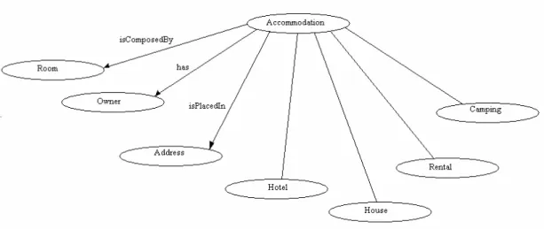
Through the entire thesis, different examples and scenarios of comparisons between ontologies will be used to illustrate the reader with the steps followed to arrive to the final result. The main example used deals with some hypothetical aspects of an accommodation. The different ontologies dealing with accommodation have some concepts in common and some different ones. At this moment we are going to introduce the ontologies of the example as they were edited with Protégé OWL.

It should be pointed out, that the first ontology introduced to our polygon method is going to be considered as the standard ontology, and the second one is going to be compared to it. This means that the similarity is going to be described as “how similar the second ontology is to the standard one”. The standard ontology receives the name of Accommodation1.

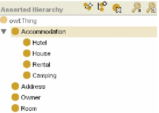
Figure 2: Classes in the Standard Ontology.

Figure 3: Properties in the Standard Ontology.

Figure 4: Individuals in the Standard Ontology.

The three main features of an ontology (classes, properties and individuals), are identified for this ontology, which is going to work as the standard one.

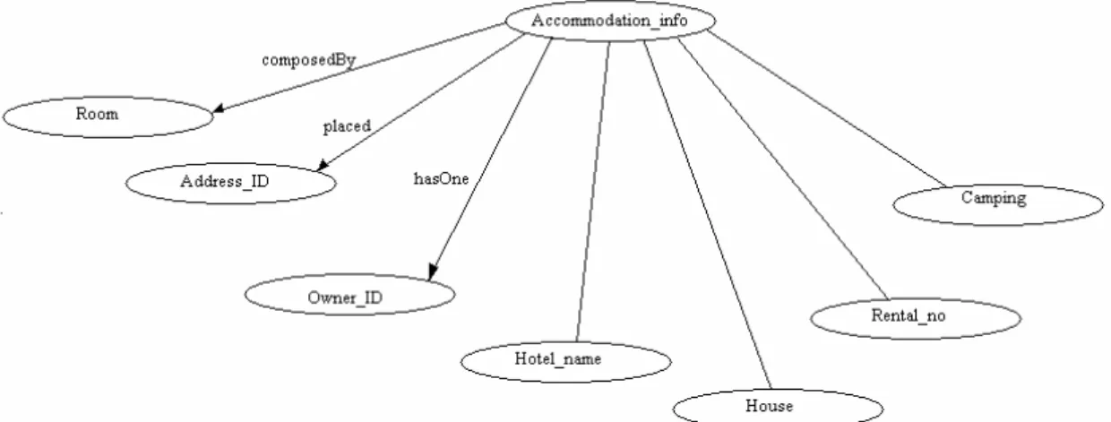
We now implement with Protégé the ontology that is going to be compared to the previous one. When referring to this ontology we are going to use Accommodation2.

Figure 5: Second Ontology.

Figure 6: Classes in the Second Ontology.

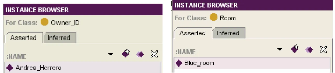
Figure 8: Individuals in the Second Ontology.

Once the implementation is done, the OWL code for each of the ontologies is also generated. In the next step we find the way to access that code with java methods.

3.3

Access the ontologies from Java: Jena

As the general requirements specify, the code of the method has to be implemented in java. The requirements also specify that the input ontologies have to be written in OWL. Consequently, OWL code has to be accessible from the java editor.

That problem is aimed by Jena, a Semantic Web Framework for Java. This open source framework used for building Semantic Web applications provides a programmatic environment for RDF, RDFS and OWL. Jena was at first developed to be a Java API for RDF, but later implementations include other functionalities such as the Jena2 ontology API.

This API provides an interface for the Semantic Web application developers. That makes it an ideal programming toolkit when we want to process the ontologies created in Protégé-OWL.

When we deal with Jena, the class Model is the one used to access the statements in

a collection of RDF data. If, in stead of accessing RDF data, OWL data has to be processed, the class OntModel is the one used. This class is an extension of the

previous Model class and makes accessible the main features of an ontology: classes,

properties and individuals. The methods included in this class provide the needed functionalities to access these features in different ways.

In order to use this class the first step is the creation of an ontology model using the Jena ModelFactory. The polygon method is going to deal with two different

ontologies in order to compare them. Therefore, there is a need to create two ontology models, one for each of them.

OntModel m1 = ModelFactory.createOntologyModel(OntModelSpec.OWL_MEM);

OntModel m2 = ModelFactory.createOntologyModel(OntModelSpec.OWL_MEM);

Accommodation1 is the source file used as input for the first model m1, while

Accommodation2 is the file issued by m2.

From now on, the ontologies will be available by using Java methods through their respective models.

At this point of the implementation we are going to take an overview of the general method we are developing.

The polygon method is based on the comparison of the features from both ontologies, the standard one and the one which is going to be compared. As it has been already pointed out, these features can be grouped into classes, properties and individuals.

Hence, classes in ontology1 have to be compared to classes in ontology2 and the same procedure has to be followed for the properties and the individuals.

There is no need to compare classes in ontology1 with properties in ontology2 and vice versa. This comparison does not add any relevant data to our study, because that would not mean that the ontologies are more similar. Therefore, the comparisons between the features are going to be restricted to the same kind of feature in both ontologies.

Moreover, subclasses will also be considered and grouped regarding their super class. Two subclasses will only be compared to each other if some similarity is found between super classes.

Once the models are created the information from each of the ontologies can be easily retrieved. We use the following methods to retrieve the existing classes, properties and individuals.

Iterator i = m1.listClasses(); i.hasNext();

OntClass c = (OntClass) i.next();

Iterator s = c.listSubClasses(true); s.hasNext();

Iterator f = m1.listObjectProperties(); f.hasNext();

Iterator s = c.listInstances(); s.hasNext();

By means of these methods the names of the features are stored, and after compared with the ones belonging to the other ontology taking into account the fact that we are only interested in comparing the corresponding groups of features. The comparisons are made in the next section of this thesis.

3.4

Comparing Strings in Ontology matching

After the information retrieval, the names of the elements corresponding to each of the ontologies are stored and converted to Java Strings.

The next step deals with the comparison of these Strings. According to those results of the comparison, the polygons can be represented, and finally, based on those representations, the final matching result can be obtained.

Comparison of strings is a much issued topic in the field of ontology research. The reason is that many different ways of comparing strings can be used, and efficiency and accurateness of the result depends on the situation and the parties involved. Nevertheless, in this study, we are going to deal with the comparison of strings oriented to Ontology matching. The examples proposed, and the cases considered will all be dealing with the names of the classes, subclasses, properties and individuals in the involved ontologies.

Moreover, there is also a great variety of methods that can be used for the comparison of ontologies and its elements. Consequently, and before taking a decision about which one to use, some studies have to be conducted in order to determine which of the existing methods has better results in the field of ontology matching.

3.4.1

Previous research

Previous studies have already conducted research about the effectiveness of the string comparing methods. According to Cohen (Cohen et al., 2003) we are going to have a classification of the methods belonging to the class SecondString.

SecondString is an open-source package of string matching methods based on the java language. These methods follow a big range of approaches and have been designed according to different criteria and perspectives, such as statistics, artificial intelligence, information retrieval, and databases.

Previous classifications divide these methods into three groups according to the methodology they use to establish the correspondence between strings: Edit-distance metrics, Token-based Edit-distance metrics and hybrid methods.

1) Edit-distance metrics

This method considers the two strings that are going to be compared. One of them is taken as the input and the other one as the output. Transformations are done between both Strings for them to be the same. The distance between both strings can be seen as the shortest sequence of edit commands that transform the input into the output. These transforming commands are copy, delete, substitute and insert.

Depending on how the cost of the editing operations is considered, two edit distance methods are regarded by the SecondString class.

The first of these methods consider that all the editing operations have unit cost and therefore, the distance increases the same independent from the edit methods used to transform the input into the output. The methods included in this modality are the Levenstein distance and Level2Levenstein distance. In the second modality, each of the transforming commands has a particular cost. That makes that depending on the parameter used; the distance between the two strings is going to increase in a different way. The methods belonging to this modality are the Monge-Elkan and the Level2Monge-Elkan.

Some similar metrics not based on the edit-distance models are Jaro, and its variants: Level2Jaro, JaroWinkler, and Level2JaroWinkler.

For these methods, the distance between two Strings is determined according to the number and order of the common characters between them.

Given strings:

s = a1, …. aK, and t = b1, ….. bL,

A character a_i in s is said to be common with t if there is a b_j = a_i in t such that i - H <= j<= i + H,

where H = min(|s|, |t|) / 2

Let s’ = a1’, …. aK’, be the characters in s which are common with t (in the same

order they appear in s) and

let t’ = b1’, ….. bL’, be the characters in t which are common with s (in the same

order they appear in t)

The definition of a transposition for s’, t’ to be a position i such that a_i’= b_i’. Let T_s’;t’ be half the number of transpositions for s’ and t’. The Jaro similarity metric for s and t is

2) Token-based distance metrics

In this metric, the strings which are going to be compared are considered as multi-sets of tokens (words).

Jaccard similarity is one of the methods included in this section. It computes the similarity between the sets of words S and T as

TFIDF (or cosine similarity method) is based on the frequency of words inside the tokens as well as the size of the core part. In order to define it, we have to define:

Where TF_w,S is the frequency of word w in S, N is the size of the “corpus” and IDF _w is the inverse of the fraction of names in the corpus that contain w. With those concepts we can define:

And finally:

Jensen and Shannon distance regards a token set as samples from an unknown distribution P_s of tokens. The distance between S and T is computed based on the distributions P_s and P_T. KL(P||Q) is the Kullback-Lieber divergence where

The distance can be defined as follows:

P_s distribution can be calculated using the function of Dirichlet or Jelenik-Mercer. That combination results into two methods: Dirichlet JS and Jelinek-Mercer JS.

Finally, Fellegi and Sunter and SFS (Simplified Fellegi and Sunter) methods can also be pointed out.

3) Hybrid methods

An important aspect of these methods to compare Strings is that they can be combined between themselves to obtain better results. When two methods belonging to different branches are combined, we obtain a hybrid method, with some characteristics from each of the modalities.

There are three hybrid methods that should be studied: SlimTFIDF, SoftTFIDF and JaroWinklerTFIDF.

3.4.2

Cases and scenarios

Once that all the methods under study have been introduced, and before a comparison between all them is made, the scenarios in which we are going to work are presented in this section.

We are going to evaluate separately the three different types of methods: edit-distance metrics, token-based edit-distance metrics and hybrid methods.

In each of the three evaluations, pairs of strings to be compared are proposed. The pairs of strings are divided into three groups:

a) Very similar pairs of strings.

b) Pairs of strings with some similarities. c) Pairs of strings with nothing in common.

Inside each of these groups, some features are going to be taken into account for the comparisons. When editing ontologies different styles can be followed for the names of the classes, properties and individuals. The sub-groups of pairs cover those differences. Some of the aspects taken into account are the differences between capital letters and lower-case, the differences between long and short words, the influence of the underscore or the influence of the spaces.

For each of these features, the different string comparing methods will be checked.

The strings used for the evaluation will try to make clear the feature tested. For that purpose, some examples and its variations will be conducted through all the tests.

Depending on the results obtained, it will be decided if a normalization process is needed before the Strings are compared to each other or not.

According to the Unicode Normalization definition the process of normalization produces one binary representation for any of the binary representations of a character. The process removes some differences but preserves the case and reduces alternate string representations that have the same linguistic meaning. Finally, we have to point out that the next section the best method will be chosen for each of the possible situations and finally one only method will be chosen for the implementation of the application.

3.4.3

Comparison of methods

We compare the methods running examples in Java. After that, we present the results in the tables at the appendixes.

It has to be pointed out that to consider two strings to have a relevant similarity the value of the similarity between them has to be higher than 60%.

The decision of that value is based on empirical practices. After reviewing examples and considering different scenarios, it is demonstrated that strings with a similarity above that value can be considered to have something in common, while strings with a similarity coefficient below that percentage are not really related to each other and the similarity can be just considered as a coincidence.

Due to that reason, pairs of strings with a similarity coefficient lower than 0.6 will not be taken into account when comparing the classes, properties and individuals in the ontologies.

In this section we analyze the results: 1) Edit-distance metrics:

The metrics included in this section are Levenstein, Monge-Elkan, Jaro and Jaro-Winkler. All of them in the simple form and in the Level2 form. That makes a total number of 8 metrics to compare. The way results are presented in each of the metrics has to be taken into account as well. Monge-Elkan, Jaro and Jaro-Winkler show the similarity with a number between 0.0, when there is any similarity, and 1.0, when the strings coincide 100%. However, Levenstein shows the similarity with a number between 0.0, meaning maximum similarity and -• meaning no similarity at all.

a) Very similar pairs of strings:

In the first one we can find the comparisons of the pairs of strings in one sense while in the other table the comparisons are made in the other direction. The position in which the strings are introduced to the comparing method affects the result for the Level2 edit distance metrics while the Level1 metrics are not influenced by the order of the strings. We will analyze that influence for different cases.

When we compare very similar pairs of strings we can make several remarks: Any of the metrics considers the influence of capital letters, regardless the length of the word or the order of the strings.

Adding a particle before or after the main word (isComposed, composedBy) Levenstein, Jaro and Jaro-Winkler consider a difference with the original word (composed). In the case of Levenstein the difference is quite big, while in Jaro and Jaro-Winkler the percentage of similarities goes down to 80.833%. Monge-Elkan considers that the strings continue with 100% similarity. For all these first examples, the order in which we place the strings for the comparison does not influence the final result.

When the particle is introduced with the underscore (is_composed,

composed_by) Levenstein considers that the similarity between them and the

original word is even smaller. Monge-Elkan is the only metric which continues considering 100% similarity between those variations and the original word. Jaro and Jaro-Winkler estimate the similarity in 78.40%, which is still a considerable similarity.

As soon as the length of the original word begins to decrease, Jaro and Jaro-Winkler do not consider the similarities to be so obvious, and when the original word has 5 or less characters (is_compo) the similarity arrives to 0%. In general, the Level2 metrics detect more differences between the strings, and show lower values for the similarities when more changes are introduced. We can say that these metrics are more sensible to changes and stricter when considering differences between strings. A good example of this can be the difference between Jaro-Winkler and Level2 Jaro-Winkler when evaluating the similarity between composed_by and composed. Jaro-Winkler estimates 94,54% while Level2 Jaro-Winkler estimates 50% similarity.

The length of the words when the particle is added with underscore does not vary the result with the Level2 metrics which continue considering 50% of similarity in all the cases (is_composed, is_compose, is_compos, is_compo,

On the other hand, when we change the order of the introduced strings, the difference between the results is remarkable. While in the first sense, the results are as we have already described, in the other sense the Level1 metrics continue with the same behavior but the Level2 metrics consider that all the pairs are 100% similar no matter the length of the word or the prefix we add with underscore.

That means that if we introduce first the original word and then its variations, the Level2 metrics consider 100% similarity between the strings, while in the other sense the percentage is always 50% no matter the length of the word. We will take into account this characteristic when taking a decision to choose one of the metrics and implementing the method.

When we consider the influence of the spaces we find the same results as the ones for the underscore. We add short particles before and after the main string (composed by, is composed) and only Monge-Elkan considers that the strings continue the same. The rest of the methods make the difference between the strings with a similarity of (78.40%, 90.90%) and in the case of Level2, the percentage goes to 50% in all the cases.

The same results are obtained when changing the order of the strings for the comparison and when reducing the length of the words.

Finally we study the difference between the underscore and the space. In this case the Level2 metrics consider that there is no difference between them and the normal metrics consider a small similarity between them (around 94%). Jaro and Jaro-Winkler have very similar results in all the cases, but we can notice that Jaro tends to be more exigent and finds more differences between the cases proposed.

As the pairs of strings compared in these two tables are considered to be very similar, the results obtained are supposed to be higher than 60% of similarity (that value will be considered as relevant). In these tables, the values under 60% are pointed out for the reader to identify easily, where the metrics do not obtain the expected result.

b) Pairs of strings with some similarities:

The comparison tables are in the appendixes 3 and 4.

In these tables we can see that the conducting example is still the same, but in this case we are going to compare the string composed with three others with some similarities (component, compound, comprehend). As in the previous table, the influence of the capital letters, the underscore, the spaces and other features are going to be studied.

When we compare just the original strings and the strings with some particle before and after it we realize that the method showing a higher similarity is Jaro-Winkler, after that Jaro, then Monge-Elkan and finally Levenstein. In all of the cases, the results do not vary from the normal metric to the Level2 metric. Changing the order of the strings introduced does not vary the results neither.

When we introduce the underscore variations, Jaro-Winkler, Jaro and Monge-Elkan still detect similarity while the Level2 metrics and Levenstein do not detect important similarities between the strings.

This results change drastically if we change the order of the strings. When the original string is introduced first and after the variations, the similarities found are higher at it happened in the previous tables.

In this case, the results from the Level1 metrics remain the same, but the results obtained from the Level2 metrics change from 40% to 70% (or even 90% in the case of Jaro-Winkler), which means that they become relevant to our study.

The same behavior is found for the spaces. Jaro-Winkler, Jaro and Monge-Elkan give always values higher than 60% with small variations between them, while the rest of the methods do not consider relevant similarities between the proposed strings.

As it happened in the previous table, the Level2 metrics do not consider similar any of the pairs of strings when one of the strings belonging to the pair includes underscore or space, but when we go to the table in 4 and we change the order of the strings, Level2 metrics consider even more similarities between the strings.

c) Pairs of strings with nothing in common:

The comparison tables are in the appendixes 5 and 6.

In these examples, we will compare the string composed to three strings with no similarity to that one: formed, integrated and organized.

No similarity should be found between the proposed pairs provided that there are not enough things in common to think that the pairs should be matched to each other in a real example. The only cases which have a similarity higher than 60% are marked in yellow to indicate that the values obtained are not the ones expected.

Jaro-Winkler, Jaro-Winkler Level2, Jaro and Jaro Level2 find similarities between two pairs of strings, when the string formed is compared.

When introducing the underscores and the spaces, all the methodologies consider that the similarity found is not relevant enough, and only Jaro and Jaro Winkler obtain a value higher than 60% in one occasion.

Level2 Jaro-Winkler and Level2 Jaro are more exigent and the similarities they find can not be considered to be relevant in any of the examples.

When we go to table 6 and consider the comparisons in the other order, we realize that more similarities are found. Without underscores or spaces, the results are the same, but when we introduce those elements Jaro and Jaro-Winkler detect similarity in 4 cases while Level2 Jaro and Level2 Jaro-Jaro-Winkler detect similarity in 10 cases.

2) Token-based distance metrics:

In this section we will analyze six different metrics based on the study of tokens. Three of them are variations from the Jensen-Shannon method. When this method is implemented with the Dirichlet function we obtain the Dirichlet JS, when it is implemented with the Jeliken-Mercer function, the obtained method is Jeliken-Mercer JS, and finally we have the Unsmoothed JS. Apart from that, we will analyze the results for the Jaccard metric, TFIDF metric and Fellegi and Sunter metric.

When regarding the way the metrics express the results, Jaccard, TFIDF and Unsmoothed JS express the similarity with values from 0,0 (no similarity) to1,0 (100% similarity). Dirichlet JS and Jeliken-Mercer JS do not result in any numeric value expressing the similarity, the only characteristic they express is the lack of similarity by means of 0,0 numeric value. The rest of the possibilities are expressed by NaN (Not a Number), which will be not useful for the aim of our study. Finally, Fellegi and Sunter metric expresses the value 0,0 when no similarity is found, and the maximum value varies depending on the length of the strings. We can point out that these metrics will not be influenced by the order of the strings. Due to that, we will have just one table for each of the three groups of pairs:

a) Very similar pairs of strings:

The comparison table is in the appendix 7.

In this case we compare the same strings as in the table for the edit distance metrics. The use of capital letters is not relevant for any of the methods, but they all consider that adding a short particle at the beginning or at the end of the string causes the total loss of similarity with the original string.

When introducing the underscore, the length of the strings is not relevant, but only TFIDF and Unsmoothed JS consider a similarity in those cases, as it happens with the use of the spaces.

The difference between the use of the underscore or the space is not appreciated by any of the methods.

b) Pairs of strings with some similarities: The comparison table is in the appendix 8.

When the pairs of strings begin to have some different aspects, the results are the same for all of the methods: any of them consider that the strings have any similarity, so all the similarity coefficients obtained are 0, for all the metrics and for all the possibilities.

c) Pairs of strings with nothing in common: The comparison table is in the appendix 9.

The same thing happens when the pairs of strings get even more different. None of the methods is able to find any similarity between them, so all the displayed results are 0.

We can conclude saying that the Token-based distance metrics are appropriate for pairs of Strings that have many aspects in common, but as soon as the examples get more and more different these methods are not able to notice the minimum aspects they have in common.

3) Hybrid methods:

It is time to analyze how hybrid methods are used in order to compare ontologies. Hybrid methods are formed by a combination of an edit-distance metric and a token-based metric. We are going to analyze 3 methods following these characteristics: Slim TFIDF, Jaro-Winkler TFIDF and Soft TFIDF. For each of them we will propose the same tables of strings already used, and the strings will be introduced in both senses in order to analyze how that affects the results.

a) Very similar pairs of strings:

The comparison tables are in the appendixes 10 and 11.

When comparing similar pairs of strings with hybrid methods, characteristics from both edit-distance metric and a token-based metric are observed.

When particles are added before and after the main string (isComposed,

composedBy), the same results are obtained in both tables: Slim TFIDF and

Jaro-Winkler TFIDF consider a very high similarity, while Soft TFIDF sees no similarity at all. When the underscore is introduced between the particle and the string (is_composed, is_com, composed_by), the three methods consider a relevant similarity, regardless the length of the string.

Only when both particles are introduced, before and after the string (is_composed_by) Soft TFIDF considers that the similarity is 0% if the original string (isComposedBy) is introduced in the second place, and the three methods consider a non-relevant similarity if the original string is introduced in the first place.

Finally, when comparing the original strings with the ones which have a particle introduced and separated by a space (is composed), all of them show relevant similarities between the pairs.

It can be pointed out that while Slim TFIDF and Jaro-Winkler TFIDF are influenced by the order of the strings, Soft TFIDF returns same results.

b) Pairs of strings with some similarities:

The comparison tables are in the appendixes 12 and 13.

The table with pairs of strings with some similarities is very revealing. In Slim TFIDF and Jaro-Winkler TFIDF the results are around 60% of similarity. It could be expected because that is the value marking the relevance of the string similarity and in this cases the similarity if the strings is relevant only in some of the cases. The unexpected is that Soft TFIDF finds 0% similarity in some of the cases, as it is considered that all of them have at list some similarities. That behavior is found regardless the length of the word, the features introduced and the order of the strings.

c) Pairs of strings with nothing in common:

The comparison tables are in the appendixes 14 and 15.

The behavior of Slim TFIDF and Jaro-Winkler TFIDF is coherent with the one we have been observing in the past tables. Both detect that the pairs of strings have few things in common so the similarity found between them is not considered to be relevant in most of the cases, except from some occasions. As it could be expected Soft TFIDF continues with the strict view and considers 0% similarity for all the pairs of strings in both senses.

3.4.4

Results

This sub section has presented the results obtained after comparing the pairs of strings. Once those results have been explained and analyzed, it is time to take a decision according to the data and decide which methods are more convenient for the comparison of ontologies at which this thesis is aimed.

1) Edit-distance metrics:

Edit-distance metrics were the ones we first compared. Among the eight methods compared, Levenstein is the one we can consider to be less appropriate for our purposes. The results are not given in percentages and after the studies made we can say that the results are not very accurate. Level2 Levenstein has the same problems found for Levenstein.

Monge-Elkan and Level2 Monge-Elkan give results included in the expected ranges. Even though, the metrics do not make differences between the different examples, and different cases have the same result. Due to this reason we can conclude that these methods do not discriminate very well between the strings and though, the results given are quite approximated.

We will focus on the four methods left: Jaro, Level2 Jaro, Jaro-Winkler and Level2 Jaro-Winkler.

The results obtained for Jaro and Jaro-Winkler are very similar, the same as the ones obtained for Level2 Jaro and Level2 Jaro-Winkler. In this situation, we will first compare the two groups of metrics: Level1 and Level2.

The first characteristic we can point out is the fact that Jaro and Jaro-Winkler consider no similarity for the strings with particles for short words (comp,

is_comp). That problem is solved by Level2 metrics, which consider 100%

similarity in all those cases in one of the senses.

Even if Level2 metrics have to make the evaluation in both senses in order to deal with all the possibilities, once that has been taken into account, the results obtained are more accurate than the ones obtained with Level1 metrics.

When we move to more different pairs of strings, Level2 metrics detect more similarities. At this point we have to take into account that ontology matching is used in the cases where the domains of the ontologies are overlapping. That means that the domains compared will have many features in common. In that situation we can conclude that Level2 metrics will give a better result due to the fact that they work better with similar strings than Level1 metrics do.

Level2 Jaro-Winkler obtains better results in some occasions so we can conclude this subsection with the conclusion that Level2 Jaro-Winkler provides the best functionality among the edit distance metrics for ontology matching.

2) Token-based distance metrics:

Once the comparison of these methods is finished we can reach the conclusion that any of them is valid for our objective. The results obtained with all of them do not consider many of the similarities needed when comparing ontologies, so we conclude saying that token-based distance metrics are not appropriate for the implementation of applications dealing with ontology matching.

3) Hybrid methods:

Hybrid methods introduce a new option with the concept of combining the two previous groups of methods.

Among the three methods presented, Soft TFIDF is the first one to be ruled out. The results obtained for the pairs of strings with some similarities show no similarity in some cases where there should be some found. Our objective is to put in common ontologies developed in distributed environments, and even if the domains issued will be the same, it is necessary to have a margin in order to regard possible pairs only with some common features.

We move then to the evaluation of Slim TFIDF and Jaro-Winkler TFIDF. The results obtained by these metrics are similar in all the situations, but when regarding very different pairs of strings we can easily observe that the results obtained by Slim TFIDF are more accurate while Jaro-Winkler TFIDF finds more similarities between some pairs of strings.

According to that fact we can say that Slim TFIDF is the most appropriate metric for our purposes, among the hybrid metrics.

Finally, we have to make the comparison between the two metrics which have been chosen as the most appropriate ones: Level2 Jaro-Winkler and Slim TFIDF. Considering the similar pairs of strings both methods have a very similar behavior, especially if we consider that when implementing the application we will take into account the maximum value found doing the comparisons in both senses.

The most important differences are found when we move to the pairs of strings with nothing in common. In this case Slim TFIDF finds fewer similarities and considers that the strings have fewer things in common. That leads to more accurate results.

We can conclude the study of the comparing methods included in the Class Second String saying that when dealing with Matching Ontologies, the most appropriate method, and therefore the one we are going to use for our application is Slim TFIDF.

3.5

From the comparison results to the polygons:

JMatLink

At the end of section 3.4, a method was chosen for the implementation of the application. Once we have made a decision on the best comparison method for editing ontologies, we can apply that method to obtain the results of the comparisons between the strings. Those results correspond to the best matching found between the two ontologies. That means that for each of the classes, properties and individuals in the standard ontology, the most similar string in the second ontology is found and matched to it.

That information is showed in a table containing the pairs found and the similarity coefficient between them.

Concerning subclasses, if two classes are found to have a relevant similarity and consequently matched to each other, it is checked if they have subclasses. If subclasses are found in both ontologies, another comparison is made between them and another table shows the similarity values between those Strings.

Therefore, there will be a table for the classes in first level, and another similarity table for each of the groups of subclasses belonging to the same super class similar to another one.

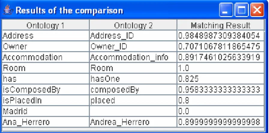
Regarding the example already proposed, when we run the application we obtain two different tables. The first table includes the similarity measures for the classes, properties and individuals, while the second one shows the similarities found for the subclasses belonging to the classes Accommodation and Accommodation_info. We can see that the pairs are matched according to the maximum similarity found and the matching result is also expressed in the third column of each table.

Figure 10: Similarity table for the comparison of subclasses.

The next step of the implementation consists on finding the general similarity coefficient of the ontologies. That is going to be done by representing polygons based on the results obtained and measure their area.

For the representation of the polygons, a software package with mathematical functions has to be used. Matlab was found to be the ideal tool for this purpose and thereby was chosen for the implementation of the software.

Matlab is a very widely extended tool with its own programming language for technical computing. Its wide use has made it connectable with many other applications. When trying to access Matlab with Java, we find that we need a library called JMatLink. Those libraries allow us to use the functions available in Matlab using the Java programming language.

In the next section we will see how the polygons are represented in Matlab according to the similarity coefficients found between the pairs of strings.

3.6

Representation of results: Matlab

Based on the information in the tables, the polygons are represented in Matlab. Many approaches can be followed in order to arrive to the final polygons. In this section the approach chosen for the application is explained.

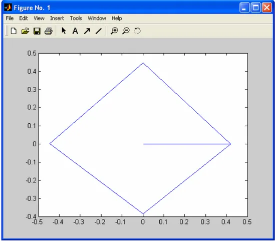
When the standard polygon has to be represented, the similarity values are not taken into account. All the points have a distance 1 to the centre of the axes. The first pair is represented by a point placed in the x axis (0º). The point for the second pair found is placed 180º from that point. The third one is placed 90º far from the first pair and the fourth one is placed 270º far from the first pair. Once the four first pairs are situated in the standard polygon we obtain four points corresponding to the four axes.

When more pairs are found, new points are added to the standard polygon. Another axis is introduced cutting in two halves the first quadrant and the perpendicular one is also added. When placing the four next points they will have a distance to the x axis of 45º, 225º, 135º and 315º, respectively.

After introducing those points, the same tasks are performed again in order to introduce new points, the 45º angle is divided in two halves and new axes are represented.

The number of points represented is equal to the number of pairs which have a relevant similarity.

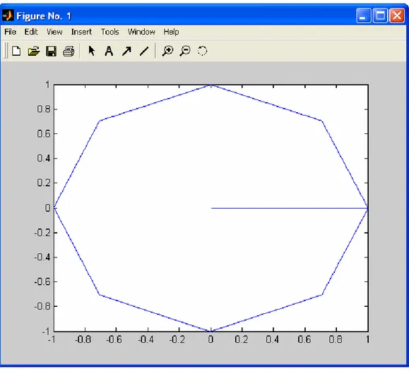
According to that procedure, when we represent the standard polygon for the table in Figure 7, we obtain the representation of eight points, providing that one of the elements in the standard ontology does not match any of the elements in the second ontology with a relevant similarity value.

The area of the standard polygon is calculated and stored in order to be used to calculate the final result.

Area1= 2.8284271247461903

Figure 11: Standard polygon.

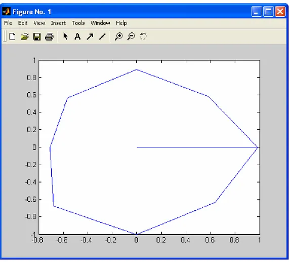
The second polygon is represented using the similarity coefficients from the table in Figure 7. Each of the points in the standard ontology, corresponding to a pair matched is multiplied by the similarity coefficient corresponding to that pair. Therefore, we obtain a polygon with the same number of vertices but a different area, varying according to the similarity values shown in the table.

The polygon for the comparison of the classes, properties and individuals and the value of its area are shown in Figure 10.

Area2= 2.2096027964711165

Figure 12: Second polygon

The second table has to be taken into account in this point of the implementation. The subclasses of Accommodation and Accommodation_info are represented in the same way.

For the standard polygon of the subclasses we introduce two multiplying factors. The first multiplying factor is related to the similarity measure of the super class. In the example, House, Hotel, Rental and Camping are subclasses of the super class

Accommodation. Accommodation is related to the class Accommodation_info with a

similarity of 0,891746. That makes that all the subclasses are going to be represented in their polygon multiplied by that factor.

The second multiplying factor depends on the level where the subclass is found. Subclasses placed closer to the original classes are considered to be more relevant for the comparison of two ontologies, while subclasses in lower levels are less relevant for the study.

Consequently, the multiplying factor for the subclasses in first level is 0,5, while the factor for the rest of the levels is the factor in the first level divided by the

According to that procedure, the resulting factors for this polygon are: 0,5*0,891746 = 0,445873.

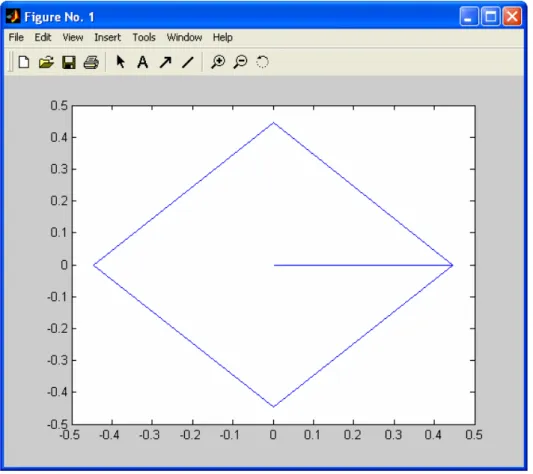
Therefore, the standard polygon for the group of subclasses found has four vertices at the points of (0, 445873,0), (0, 0,445873), (- 0,445873, 0), and (0, - 0,445873).

Area1 subclasses= 0.39760555571849976

Figure 13: Standard polygon for the group of subclasses.

When the second polygon has to be represented for the group of subclasses, the value of each point in the standard polygon is multiplied by the corresponding similarity value.

By that simple operation, the area of the second polygon varies once more and the second polygon is obtained.

Camping – Camping 1,0. Rental – Rental_no 0,9428.

When multiplying those values by the factors that we already had, the resulting values are

House – House: 1,0*0,5*0,891746=0,445873. Hotel – Hotel_name: 0,8662*0,5*0,891746=0,3862. Camping – Camping: 1,0*0,5*0,891746=0,445873. Rental – Rental_no: 0,9428*0,5*0,891746=0,42069.

Representing those distances in the correct axes we obtain the polygon and its area.

Area2 subclasses= 0.36039777842757076

Figure 14: Second polygon for the group of subclasses.

When all the areas of the polygons have been stored, the final value can be calculated.

Areas corresponding to the standard ontologies are added together, as well as areas corresponding to the non-standard ontologies.

Area1 Total = 2.8284271247461903 + 0.39760555571849976. Area2 Total= 2.2096027964711165 + 0.36039777842757076. The similarity value is:

We can conclude that the similarity between ontology 1 and ontology 2 is: 0.8925493312983556

0.8925493312983556 0.8925493312983556 0.8925493312983556....

4

Conclusion and Discussion

In this section of the thesis, some other methods for ontology matching will be studied and compared to the polygon method. According to the results achieved, some future work will be proposed.

As we have already said, the ontology community has developed various strategies for ontology matching, according to different approaches. Many classifications have also been made for these strategies, tools and methods depending on the aspect of the ontology compared, the input received, the result given, etc.

One of the most famous classifications groups the strategies for matching ontologies into de following groups:

- Hierarchical clustering techniques. - Formal concept analysis.

- Analysis of terminological features of concepts and relations. - Analysis of structure.

All of these methodologies are motivated by the same fact: the distributed ontology development. Distributed organizations and communities develop ontologies covering different domains. The problem comes when two or more ontologies cover overlapping domains and we need to put them in common. In that moment, some technique has to be used: ontology matching, ontology alignment, ontology merging, etc.

The election of the approach and the method varies from one community to another. Therefore, it is interesting to consider solutions given to the problem from different points of view.

Six different methods are presented in order to give a general view about the possibilities to solve the problem presented above.

4.1

Method 1: GLUE.

According to Doan, Madhavan, Domingos and Halevy (Doan, Madhavan, Domingos & Halevy, 2003) GLUE solves the problem of finding semantic mappings, given two ontologies to ensure interoperability between them.

This method uses learning techniques to semi-automatically create semantic mapping between ontologies. The key step consists on looking for semantic correspondence. This technique is still conducted by hand, which means an important bottleneck in building large scale information management systems. For GLUE, the ontologies are organized in taxonomy trees. Each of the nodes in the trees represents one concept and each of these concepts has associated a set of instances and a set of attributes.

The matching procedure consists on mapping between taxonomies. For each of the concepts in one taxonomy the most similar concept node in the other taxonomy is found.

GLUE uses the joint probability distribution to compute the similarity within the multi-strategy learning approach. This approach combines a set of learners and their predictions with some domain constraints and heuristics in order to obtain matching accuracy.

When taking a closer look to the implementation we distinguish the following steps: In the first step, the distribution estimator takes two ontologies as an input, including their structure and data instances. For every pair of concepts in the ontologies the learning techniques compute the joint probability distribution. After that, those numbers go to the similarity estimator, which applies similarity functions and obtains the similarity matrix. In the final step, the relation labeler takes the matrix, domain specific constraints and heuristics and obtains the final mapping configuration as an output.

This method is evaluated in three real world domains in order to evaluate the matching accuracy. A high accuracy was obtained (from 66% to 97%) but some problems were still found: there was not enough training data, the learners used were not appropriate and some nodes were considered to be unambiguous.

This method has been placed in the first position considering the similarities with the polygon method. Both of them follow the same schema of comparisons. In GLUE, all the possible pairs of concepts are made, and then the similarity between them is evaluated. A matrix is formed with those values and finally the highest value shows which concepts are more likely to be matched together.