Marginal cost of railway infrastructure wear and tear for freight and
passenger trains in Sweden
Mats Andersson
Swedish National Road and Transport Research Institute (VTI) Department of Transport Economics
Box 920 781 29 Borlänge
Sweden
Tel.: + 46 243 44 68 66
E-mail address: mats.andersson@vti.se
Manuscript version: November 30, 2009
Abstract
We analyse maintenance cost data for Swedish railway infrastructure in relation to traffic volumes and network characteristics, and separate the cost impact from passenger and freight trains. Lines with mixed passenger and freight traffic, and dedicated freight lines are analysed separately using both log-linear and Box-Cox regression models. We find that for mixed lines, the Box-Box-Cox specification is preferred, while a log-linear model is chosen in the case of dedicated freight lines. The cost elasticity with respect to output is found to be higher for passenger trains than for freight trains. From a marginal cost pricing perspective, freight trains are currently over-charged, while passenger trains are under-charged.
Keywords: Railway, Maintenance, Box-Cox, Marginal Cost
1. Introduction
There has been increasing European attention to the issue of marginal costs of railway infrastructure wear and tear in the last decade. European rail infrastructure administrations have great interest in these marginal cost estimates as they are an important corner-stone of the European transport pricing policy (European Parliament, 2001). Following the paper by Johansson and Nilsson (2004) on railway infrastructure maintenance costs, there is now research ongoing in several European countries (Lindberg, 2006).
The general approach is to do regression analysis on maintenance costs and control for infrastructure characteristics and traffic volumes. The majority of recent studies use an aggregate measure of output of the track, which is expressed in total gross tonnes of traffic consisting of both passenger and freight trains. Furthermore, log-linear models are dominating the research.
The Swedish Rail Administration (Banverket) is responsible for railway access charges in Sweden. The current charge for infrastructure wear and tear is Swedish Krona (SEK) 0.0029 per gross tonne kilometre as a flat rate for all users (Banverket, 2008).1 To increase efficiency in current pricing schemes, introducing differentiated track access charges has been discussed, based on wear and tear from different vehicle types. The hypothesis is that freight and passenger trains deteriorate the infrastructure differently, inducing different levels of cost and therefore should be priced accordingly. The reason for this position is that freight and passenger trains generate different forces on the railway track through differences in speeds, axle loads, suspensions etcetera as well as require different track quality levels. This issue has also received some attention in Sweden in a report on differentiated access charges by track engineers at the Royal Institute of Technology (KTH) and Banverket (Öberg et al., 2007).
Whether this standpoint can be supported by empirical, econometric work is yet to be revealed, but work by Gaudry and Quinet (2009) indicates that there might be substantial differences in wear and tear, not only between freight and passenger trains, but also within the group of passenger trains. Furthermore, they advocate in favour of the Box-Cox model as an alternative to previously used log-linear models. To be able to analyse the question of differentiation, the aggregate measure of traffic volume has to be abandoned in favour of a model where different traffic categories are used as outputs.
In this paper, we analyse a four-year data set on Swedish railway maintenance costs in order to contribute to the analysis on differentiated marginal costs. The purpose is threefold. First, we are interested in separating gross tonnes for freight and passenger trains in order to see if cost elasticities and marginal costs are different for the two traffic categories. Second, the choice between logarithmic and Box-Cox transformation of the data will be analysed. Third, lines with a mixed passenger and freight traffic pattern will be separated from lines dedicated to freight traffic only to see if there are systematic differences in freight marginal costs between these track types.
The paper is structured as follows. A short overview of recent work is given in section 2 followed by a description of the data in section 3. Model specifications and results from the econometric analyses with marginal cost calculations are given in section 4 and 5 respectively. In section 6, we discuss our results and draw conclusions.
2. Literature review
The issue of estimating cost functions for railway organisations has a long history and can be found as early as the 1960’s (Borts, 1960). The focus of the early research was to check for inefficiencies in the U.S. railroad industry and to regulate monopoly prices in the presence of economies of scale (Keeler, 1974).
Recent European studies have a different perspective as they are looking at the cost structure in vertically separated rail infrastructure organisations to derive short run marginal costs. These studies have grown out of a sequel of research projects on transport infrastructure pricing funded by the European Commission, such as Pricing European Transport Systems (PETS) (Nash and Sansom, 2001), UNIfication of accounts and marginal costs for Transport Efficiency (UNITE) (Nash, 2003) and Generalisation of Research on Accounts and Cost Estimation (GRACE) (Nash et al., 2008). This work is part of the CATRIN (Cost Allocation of TRansport INfrastructure cost) project currently in progress.
The study that initiated most of the current work is Johansson and Nilsson (2004) who estimate rail infrastructure maintenance cost functions on data from Sweden and Finland from
the mid 1990’s. They apply a reduced form of the Translog specification suggested by Christensen et al. (1973) using total gross tonnes as output of the track, controlling for infrastructure characteristics, but excluding factor prices. The analysis builds on the assumption that costs are minimised for a given level of output. Cost elasticities and marginal costs are given as main results.
Railway infrastructure maintenance cost functions have since then been estimated in Austria (Munduch et al., 2002), Norway (Daljord, 2003), Finland (Tervonen and Idström, 2004), Switzerland (Marti and Neuenschwander, 2006), Sweden (Andersson, 2006, 2007a and 2008) and the UK (Wheat and Smith, 2008). All of these studies use log-linear model specifications and also an aggregate measure of output, i.e. total gross tonnes. Pooling annual data for several years is done in all cases, except for Andersson (2007a and 2008) who uses panel data techniques.
Considering the variation between the individual studies, the results have been reasonably similar in terms of cost elasticities with respect to output, when controlling for the cost base included (Wheat, 2007). There is evidence for the maintenance cost elasticity with respect to output of gross tonnes to be in the range of 0.2 - 0.3, i.e. a 10 percent change in output gives rise to a 2 - 3 percent change in maintenance costs. Marginal costs on the other hand vary between countries and are more difficult to compare.
The only alternative econometric approaches so far to the one suggested by Johansson and Nilsson (2004) are found in Gaudry and Quinet (2009) and Andersson (2007b). Gaudry and Quinet (2009) use a very large data set for French railways in 1999, and explore a variety of unrestricted generalised Box-Cox models to allocate maintenance costs to different traffic classes. They reject the Translog specification as being too restrictive on their data set, which indicates that a logarithmic transformation of the data is not as efficient as using a Box-Cox transformation. Andersson (2007b) uses survival analysis on rail renewal data to derive marginal costs.
3. The data
The available data set consists of some 185 track sections with traffic (freight and/or passenger) that we observe over the years 1999 - 2002. A track section is a part of the network, normally a link between two nodes or stations that varies in length and design. Maintenance costs are derived from Banverket’s financial system and cover all maintenance activities. Both corrective and preventive maintenance are included, but winter maintenance (snow clearing and de-icing) is excluded. Major renewals are also excluded, but the data might include minor replacements considered as spot-maintenance. Infrastructure characteristics are taken from the track information system at Banverket and traffic volumes are collected from various Swedish train operating companies. Each track section contains information on annual maintenance costs (ccm_tot)2, traffic volumes (density) expressed as gross tonnes3 for freight (fgt) and passenger trains (pgt) as well as a range of infrastructure characteristics. These are track kilometres (bis_tsl), track section length-to-distance ratio4 (ld_ratio), length of switches (swit_tl), average rail age (rail_age), average switch age (swit_age), number of joints (joints), average rail weight (rlwgh) and average quality class (qc_ave).
We have split the original data set into two parts. One part contains tracks with mixed traffic and the other, tracks dedicated to freight trains only. The reason for this is the
2
Costs are expressed in SEK and 2002 price level.
3
The density definition is Gross tonne kilometres divided by Track kilometres.
4
underlying idea behind the marginal cost calculation and differentiation. Tracks without any passenger traffic are significantly different from tracks with mixed traffic from an engineering point of view. This has to do with the alignment and design of the track to deal with different train types running at different speeds with different loads. A dedicated freight line can be aligned to minimise deterioration and cost from a freight train, while the alignment for a mixed line has to be a compromise between the needs for both freight and passenger trains. In a mixed situation, freight trains will normally run at lower speeds and weights than passenger trains leading to freight trains “hanging” on the inner rail in curves, while passenger trains will “push” towards the outer rail. The super-elevation (cant) of the track is therefore non-optimal for both. Introducing a change in passenger traffic (running the first passenger train) on a dedicated freight line would therefore not give rise to a marginal change in costs, but rather a leap in costs to adjust the alignment to the mixed situation as well as covering the costs from the passenger train. Our position is that dedicated lines are better off to be analysed separately and these results will be presented alongside results of mixed lines. Analysing the introduction of passenger trains on dedicated freight lines though is beyond the scope of this paper.
The mixed line data set covers 648 observations, i.e. around 160 track sections over four years, and our dedicated freight line data set contains 101 observations (around 25 track sections).
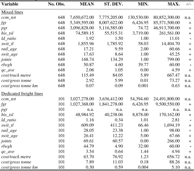
Table 1: Descriptive statistics
Variable No. Obs. MEAN ST. DEV. MIN. MAX. +/-
Mixed lines ccm_tot 648 7,650,672.00 7,775,205.00 130,530.00 80,852,300.00 n.a. fgt 648 5,349,595.00 8,007,622.00 6,426.95 85,571,500.00 + pgt 648 3,096,828.00 5,116,585.00 74.72 46,913,700.00 + bis_tsl 648 74,589.15 55,515.31 3,719.00 261,561.00 + ld_ratio 648 1.92 1.50 1.00 11.01 - swit_tl 648 1,855.96 1,785.92 58.03 14,404.70 + rail_age 648 17.21 9.59 2.00 60.66 + swit_age 648 17.63 8.64 1.00 45.25 + joints 648 168.74 134.29 1.00 799.00 + rlwgh 648 50.87 4.60 39.77 60.00 - qc_ave 648 2.06 1.05 0.00 4.59 +
cost/track metre 648 115.49 84.05 5.89 667.47 n.a.
cost/gross tonne 648 2.92 5.99 0.01 73.27 n.a.
cost/gross tonne km 648 0.07 0.09 0.001 0.63 n.a.
Dedicated freight lines
ccm_tot 101 3,027,278.00 3,636,412.00 54,394.60 24,491,800.00 n.a.
fgt 101 1,027,368.00 1,841,278.00 6,426.95 9,500,550.00 +
pgt 101 n.a. n.a. n.a. n.a. n.a.
bis_tsl 101 48,984.92 40,238.06 8,878.00 170,162.00 + ld_ratio 101 1.16 0.34 1.01 2.81 - swit_tl 101 609.09 411.23 66.46 1,694.19 + rail_age 101 28.05 23.38 1.00 98.00 + swit_age 101 26.41 12.22 5.00 67.66 + joints 101 69.61 60.57 0.00 266.00 + rlwgh 101 44.79 4.90 32.00 60.00 - qc_ave 101 3.54 0.64 1.44 4.94 +
cost/track metre 101 63.70 76.92 1.23 656.72 n.a.
cost/gross tonne 101 7.89 11.03 0.18 88.26 n.a.
A descriptive summary of the two data sets is given in table 1 and there are some differences between the two data sets worth pointing out:
• Average annual spending on maintenance per track metre is close to two times higher on mixed lines, but almost three times higher on dedicated lines per gross tonne. • Average freight traffic density is 5 times higher on mixed lines.
• There are two times more switches per track kilometre on mixed lines.
• Both switches and rails on dedicated freight lines are on average more than 10 years older than on mixed lines.
• Average track quality is much lower on dedicated freight lines.
The +/- column indicates our a priori expectation about the relationship between each variable and maintenance costs. Hence, higher values of freight and passenger gross tonnes, track section length, switches, rail and switch age, joints and quality class5 are expected to increase maintenance costs, other things equal. A higher length-to-distance ratio means easier access to the track and would lead to more efficient work schedules and reduced costs. Higher rail weight resists wear and tear and leads to less maintenance.
4. The econometric approach
We have pointed out above that knowledge of marginal costs is essential to European railway administrations. Among the available methods to estimate the marginal costs, we will use an econometric approach, i.e. an application of statistical methods to economic data. To estimate a cost function, we build on the duality between production and costs under the assumption that costs are minimised for a given level of output and input of factor prices.
We can describe the relationship between maintenance costs (C), a vector of outputs (q) and a vector of factor prices (p) as
C = f (q, p)
For our analyses, we have reasons to believe that the spatial variation in factor prices, i.e. labour, energy and capital costs over the Swedish rail network is negligible. This idea was first suggested by Johansson and Nilsson (2004) with the argument that the Swedish labour market agreements are heavily regulated at a national level. Another reason is that the majority of the track work during these years is done in-house by the Production Division of Banverket. We will therefore exclude the factor price vector p in our estimated cost functions and proceed with the assumption of equal factor prices over the network.
However, output in terms of traffic volumes is not the only factor that can influence the variation in costs over a rail network. As output varies over the network, so do the technical characteristics of the track, climate and managerial skills, which need to be controlled for. Thus, we will assume that there is a relationship between costs for infrastructure maintenance (C), and the level of output (q) given other characteristics of the infrastructure (x) and dummy variables (z);
C = f (q, x, z).
5
A log-linear regression model in form of this relationship is given in expression (1), where i denote observations, t time, k, m and n are the number of output, infrastructure and dummy variables respectively in the model. α, βk, δm and γn are parameters to be estimated. ε is the
error term assumed NID (0, σ).
it n nit m mit k kit it q x z C =lnα +ln β +ln δ + γ +ε ln (1)
The cost elasticity in the log-linear model is the derivative of the cost function with respect to the variable of interest. If the model does not include higher-order or interaction terms, the k elasticities for our output variables are expressed in general form as
LL k k k q C/ ln βˆ φˆ ln ∂ = = ∂ . (2)
These elasticities are constant over the range of output we analyse, but including higher order terms or interactions will lead to non-constant elasticities. Exact elasticity expressions will be given under the detailed specifications in the following chapter.
The log-linear model above imposes a restriction on our model as it assumes that the most efficient transformation of our data is logarithmic. An alternative to the logarithmic transformation is the Box-Cox regression model, making use of the formula for variable transformation by Box and Cox (Greene, 2003).
λ λ λ / ) 1 ( ) ( = w − w (3)
For λ to be defined for all values, w must be strictly positive. The direct benefit of using the Box-Cox transformation is that it includes the log transformation as a special case. Hence, if our data are log normal, the transformation parameter λ will be insignificant from zero. If not, the log transformation in model (1) will not be an efficient way of treating our data.
The econometric specification in general form, using a common transformation parameter for both the left and right hand side is given in (4)
it n nit m mit k kit it q x z C(λ) =α + (λ)β + (λ)δ + γ +ε . (4)
Output (q) and infrastructure (x) variables are transformed, while the intercept, variables with genuine zeros and dummy variables (z) are left non-transformed. The elasticity in the Box-Cox model (4) also includes the estimated transformation parameter λ and the general expression is C B kit it kit k kit it C q q C ⎟⎟ = − ⎠ ⎞ ⎜⎜ ⎝ ⎛ = ∂ ∂ β φ λ ˆ ˆ ln / ln . (5)
Hence, the elasticity in a Box-Cox model will be non-constant and vary with output and cost level. For a derivation of the elasticity, see Appendix 1.
5. Econometric specifications and results
In this section, we present the econometric specifications and results, including elasticities and marginal cost calculations. We start by looking at a model for mixed lines followed by a dedicated freight line model. All estimations are done using Stata 9 (StataCorp, 2005).
5.1. Mixed lines
As the Box-Cox model includes the log-linear model as a special case, we have initially estimated a Box-Cox regression model on all track sections with mixed traffic (648 observations). The model includes output of both freight (fgt) and passenger (pgt) gross tonnes per annum. Apart from that, we control for length-distance ratio (ld_ratio), track section length (bis_tsl), switches (swit_tl), rail age (rail_age) and switch age (swit_age). These are all transformed variables. Non-transformed variables are joints (joints), average quality class (qc_ave) and dummy variables for 3 years, 15 track districts and stations. The model specification is given below (6) and the estimated model in table 2 (dummy variables excluded). it it it m m it n n it it it it it it it it it it station district year joints ave qc age swit age rail tl swit tsl bis ratio ld pgt fgt C ε ω η γ β β β β β β β β β α λ λ λ λ λ λ λ λ + + + + + + + + + + + + + =
∑
∑
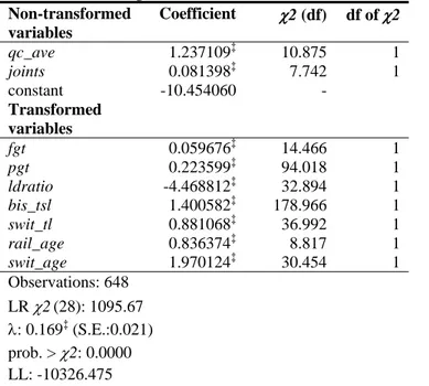
= = 1 15 1 3 1 9 8 ) ( 7 ) ( 6 ) ( 5 ) ( 4 ) ( 3 ) ( 2 ) ( 1 ) ( _ _ _ _ _ _ (6)Table 2: Box-Cox regression model estimates – Mixed lines Non-transformed variables Coefficient χ2 (df) df of χ2 qc_ave 1.237109‡ 10.875 1 joints 0.081398‡ 7.742 1 constant -10.454060 - Transformed variables fgt 0.059676‡ 14.466 1 pgt 0.223599‡ 94.018 1 ldratio -4.468812‡ 32.894 1 bis_tsl 1.400582‡ 178.966 1 swit_tl 0.881068‡ 36.992 1 rail_age 0.836374‡ 8.817 1 swit_age 1.970124‡ 30.454 1 Observations: 648 LR χ2(28): 1095.67 λ: 0.169‡ (S.E.:0.021) prob. > χ2: 0.0000 LL: -10326.475
Legend: ‡ Significant at 1% level; † Significant at 5% level; * Significant at 10% level.
All coefficients are significant at the 1 percent level (except some of the track district dummy variables). Our a priori expectations of the signs of the coefficients for these variables are given in table 1 and all estimated coefficients fulfil expectations. There are positive relationships between maintenance costs and output levels, track section length, switches, rail and switch age, joints, quality class and station areas. Conversely, costs are negatively related
to the length-distance ratio. These findings are in line with what has previously been found in Andersson (2006).
The estimate of λ, the transformation parameter, is 0.17 and significantly different from zero at the 1 percent level. Hence, we reject the logarithmic transformation of our dependent and transformed independent variables.
Table 3 summarises the estimated Box-Cox elasticities, evaluated at the sample means for output and maintenance costs using expression (5). Standard errors are adjusted using a cluster indicator for track sections, i.e. independence is assumed between track sections, but not within. A challenging result is that the mean cost elasticity with respect to passenger traffic volumes is more than three times higher than the equivalent elasticity for freight. The confidence intervals are not overlapping, indicating a significant difference at the 5 percent level. In other words, passenger trains seem to drive maintenance costs more than freight trains, which is not in accordance with conventional wisdom among track engineers. Axle load is a key variable when estimating track damage (Öberg et al., 2007), and freight vehicles are normally run with higher axle loads.
Table 3: Cost elasticities – Box-Cox
Elasticity Observations Mean Std. Error^ [95% Conf. Interval]
Freight 648 0.052264 0.001134 0.050026 0.054503
Passenger 648 0.179364 0.003643 0.172443 0.186285
^ Cluster adjusted
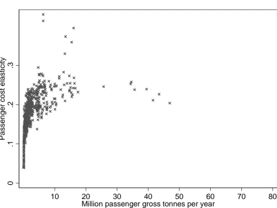
Figures 1 and 2 contain plots of track section specific elasticities derived from the Box-Cox model using expression (5). We find increasing elasticities with output, but at a decreasing rate. This shape has also been found in previous work by Andersson (2007a) on Swedish railway maintenance costs and by Link (2006) on German motorway renewal costs.
0 .0 5 .1 .1 5 F re ig h t co st e la st ici ty 10 20 30 40 50 60 70 80
Million freight gross tonnes per year Figure 1: Cost elasticity w r t freight volumes – Box-Cox
0 .1 .2 .3 Pa sse n g e r co st e la st ici ty 10 20 30 40 50 60 70 80
Million passenger gross tonnes per year
The estimated elasticities from specification (6) give us reason to also consider interaction variables, variables that will capture the joint effect from two variables. Introducing interaction variables though, has no significant impact on the results in table 2 and 3.
5.2. Dedicated freight lines
In line with the analysis of mixed lines, we have initially estimated a Box-Cox model, but the likelihood ratio test has not rejected the transformation parameter λ being zero. We therefore specify a log-linear model for dedicated freight lines. This model is built on 101 observations and some of the variables used for mixed lines are excluded. Switches, age variables, quality class and joints have proven insignificant, but we use rail weight (rlwgh) as a proxy variable for track quality instead. We also include a squared term for output to capture a potential non-linear relationship. The final model specification is given in (7).
it it n n it it it it it it it year rlwgh rlwgh tsl bis ratio ld fgt fgt C ε γ β β β β β β α + + + + + + + + =
∑
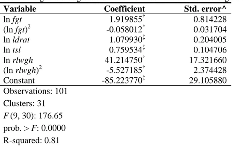
= 3 1 2 6 5 4 3 2 2 1 ) (ln ln _ ln _ ln ) (ln ln ln (7)The estimated model is given in table 4 (dummy variables excluded). The signs of the coefficients are in line with our a priori expectations except for length-to-distance ratio, which is now positive. This indicates that costs increase rather than decrease with more meeting points and double tracks.
Table 4: Log-linear regression model estimates – Dedicated freight lines
Variable Coefficient Std. error^
ln fgt 1.919855† 0.814228 (ln fgt)2 -0.058012* 0.031704 ln ldrat 1.079930‡ 0.204005 ln tsl 0.759534‡ 0.104706 ln rlwgh 41.214750† 17.321660 (ln rlwgh)2 -5.527185† 2.374428 Constant -85.223770‡ 29.105880 Observations: 101 Clusters: 31 F(9, 30): 176.65 prob. > F: 0.0000 R-squared: 0.81
Legend: ‡ Significant at 1% level; † Significant at 5% level; * Significant at 10% level. ^ Robust and cluster adjusted standard errors.
Table 5 summarises the estimated cost elasticity, evaluated at the output mean using expression (8). LL fgt fgt mean fgt fgt C/ ln βˆ 2 βˆ (ln ) φˆ ln ∂ = ln + ⋅ (ln )2 ⋅ = ∂ . (8)
Table 5: Cost elasticity – Dedicated freight lines
Elasticity Observations Mean Std. Error^ [95% Conf. Interval]
Freight 101 0.438207 0.079664 0.275513 0.600902 ^ Cluster adjusted
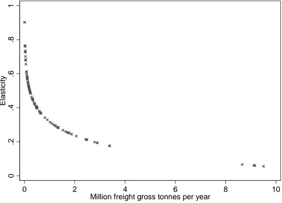
The estimate is substantially higher than the freight elasticity in the Box-Cox model. Figure 3 gives a plot of the elasticity function and it is downward sloping as opposed to upward for the mixed line elasticities.
0 .2 .4 .6 .8 1 El a st ici ty 0 2 4 6 8 10
Million freight gross tonnes per year
Figure 3: Cost elasticity w r t freight volumes – Dedicated freight lines
5.3 Average and marginal cost estimates
The elasticities derived in sections 5.1 and 5.2 are important inputs in the calculation of marginal costs. The cost elasticities of output are expressed per gross tonne (q), but from a pricing perspective, we also prefer the marginal cost to be distance related and expressed in terms of gross tonne kilometres (qgtk). Following Johansson and Nilsson (2004), for output k we express the marginal maintenance cost (9) as
gtk k it gtk k k gtk k gtk k gtk k k q C q C q C q C q C q C MC ⋅ = ⋅ ∂ ∂ = ⋅ ∂ ∂ = ∂ ∂ = φ ln ln ln ln . (9)
Marginal cost is the product of the cost elasticity φ and average cost. By this, we assume that the cost is unaffected by line length at the margin. Estimates of track section marginal costs can be derived by using the output (k) specific elasticity estimates and predicted costs as in (10)
gtk kit j it j kit j kit q C MC ˆ ˆ ⋅ =φ , (10)
where j indicates mixed or dedicated lines. The calculated marginal costs from (10) are observation specific. In order to adjust for the variation of marginal costs over track sections, we can calculate a weighted average marginal cost. We use the output of each traffic category as a track section weight in relation to total output per category. Estimates of marginal costs from track sections with high traffic levels are given a higher weight than marginal costs from track sections with less traffic.
∑
∑
⎥ ⎥ ⎦ ⎤ ⎢ ⎢ ⎣ ⎡ ⋅ = kit kit km kit km kit j kit j k q q MC WMC (11)This allows the infrastructure manager to use a unit rate for wear-and-tear over the network, and still be revenue neutral to using track section specific marginal costs.
Table 6: Average costs
Average cost Observations Mean Std. Error^ [95% Conf. Interval]
Mixed freight 648 0.682289 0.269658 0.150024 1.214554
Mixed passenger 648 5.609661 2.011954 1.638362 9.580960 Dedicated freight 101 0.224562 0.035756 0.151540 0.297585 ^ Cluster adjusted
The predicted average maintenance cost (AC) is given in table 6. AC is defined as predicted maintenance cost divided by the output specific gross tonne kilometres. The average maintenance cost per gross tonne km for mixed lines is approximately SEK 0.68 for freight and SEK 5.60 for passenger, while for dedicated lines it is SEK 0.22.
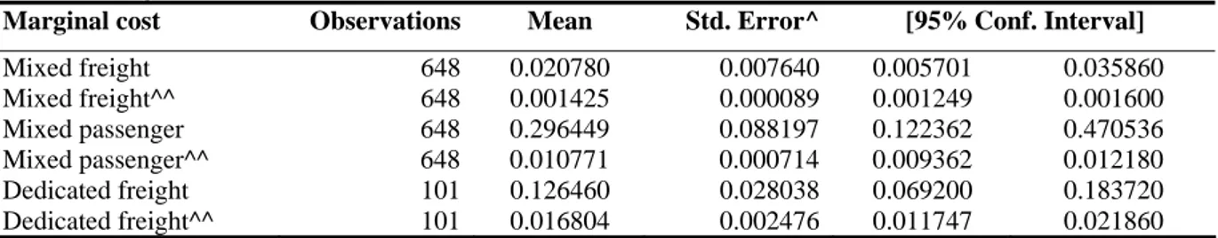
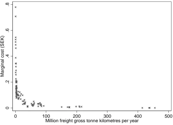
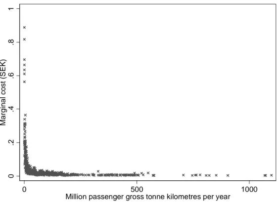
The estimated marginal costs are given in table 7. Mean marginal cost for dedicated lines is SEK 0.126. An output-weighted mean estimate is SEK 0.0168. The marginal cost for freight trains in the Box-Cox model (6) is SEK 0.021 and SEK 0.0014 as a weighted estimate. For passenger trains, the equivalent estimates are SEK 0.296 and SEK 0.0108. We observe some high marginal costs in all three cases for low volume track sections, which drive up the mean values. The marginal costs for dedicated freight lines are plotted in figure 4, and for mixed lines in figures 5 and 66.
Table 7: Marginal costs
Marginal cost Observations Mean Std. Error^ [95% Conf. Interval]
Mixed freight 648 0.020780 0.007640 0.005701 0.035860 Mixed freight^^ 648 0.001425 0.000089 0.001249 0.001600 Mixed passenger 648 0.296449 0.088197 0.122362 0.470536 Mixed passenger^^ 648 0.010771 0.000714 0.009362 0.012180 Dedicated freight 101 0.126460 0.028038 0.069200 0.183720 Dedicated freight^^ 101 0.016804 0.002476 0.011747 0.021860 ^ Cluster adjusted; ^^ Weighted estimate
0 .2 .4 .6 .8 Ma rg in a l co st (S EK) 0 100 200 300 400 500
Million freight gross tonne kilometres per year
Figure 4: Marginal costs - Dedicated freight lines
0 .2 .4 .6 .8 Ma rg in a l co st (S EK) 0 1000 2000 3000
Million freight gross tonne kilometres per year
0 .2 .4 .6 .8 1 Ma rg in a l co st (S EK) 0 500 1000
Million passenger gross tonne kilometres per year
Figure 6: Marginal costs - Passenger trains - Mixed lines
6. Discussion and conclusions
There has been increasing European attention to the issue of marginal costs of railway infrastructure wear and tear in the last decade. In this paper, we have analysed maintenance cost data for Swedish railway infrastructure in relation to traffic volumes and other characteristics, and separated the cost impact from passenger and freight trains. Furthermore, we have analysed the choice between logarithmic and Box-Cox regression models and finally checked for differences between railway lines with a mixed passenger and freight traffic pattern and lines dedicated to freight traffic only.
The analysis shows that a Box-Cox regression model is preferred for lines with mixed traffic, but the log-linear model is not rejected for dedicated freight lines. We observe that most coefficients follow our a priori expectations in terms of cost drivers for both dedicated and mixed lines. One feature though is that the sign of the coefficient for length-distance ratio variable goes from negative (mixed lines) to positive (dedicated freight lines). This seems a little confusing at a first glance as a higher ratio indicates higher track availability and larger potential for track possession times. There is a probable explanation though. The dedicated freight lines have fairly low traffic levels, which mean that there is no direct benefit in having multiple tracks with regards to available track time. Hence, track time for maintenance is no scarcity on low-volume lines, and adding more tracks to a low-volume line will generate costs. Adding more tracks to a high-volume track on the other hand will reduce maintenance costs as track availability is increased with lower costs as a bonus (less time is spent establishing, re-establishing and waiting during a maintenance activity).
The most challenging result is the ratio between the passenger and freight elasticities in the mixed line case. The freight elasticity (0.05) in the model for mixed lines is well below, while
differ from what we have previously considered as conventional (Andersson, 2007a and 2008), namely SEK 0.006 – 0.007 per gross tonne kilometre using total gross tonnes as output and panel data estimators. Freight marginal costs are well below this level and also lower than what is currently charged for wear and tear. Conversely, passenger marginal costs are almost twice of what is previously found and four times the current charge. A suggested explanation to the high passenger elasticity is to look at track management behaviour and rules. Passenger trains operate at higher speeds and require a high-quality track with tougher intervention levels compared to freight trains. This implies more frequent maintenance activities on a mixed line than on a line dedicated to freight only. Management documents at Banverket corroborate this view. Inspection class is a function of speed and gross tonnes (Banverket, 2000). Tamping levels are a function of comfort classes, which are based on quality classes. Higher speeds generate lower tolerance levels in these quality classes (Banverket, 1997). The cost elasticity is then not solely based on physical wear and tear, but on a combination of wear and tear, and ride comfort. Maintenance policies and actions are highly passenger train service orientated in Sweden and this is reflected in the cost structure as well as in train service punctuality statistics. Passenger trains are given priority to freight trains in delay situations.
This said, it can also be a matter of omitted variable bias, a common problem in regression analysis. Previous work by Andersson (2007a and 2008) has used fixed effect (FE) estimation on the same data set, using an aggregate output of freight and passenger train volumes. FE estimation solves the omitted variable bias problem if track specific characteristics are time-invariant (Wooldridge, 2002). We are not aware of any FE applications in a Box-Cox framework, but this would be one way of extending this research. Another extension is along the line of acquiring more data, inter alia speeds and axle loads, which are currently not available to us. These variables are used in the deterioration models by Öberg et al. (2007), which allocate freight and passenger train damage to the track.
There is also a difference between the elasticity found for freight trains on dedicated lines and what has previously been found. A 10 percent change in freight traffic on a dedicated line would change maintenance costs by 4.4 percent. The magnitude of the elasticities in previous models (Andersson, 2006, 2007a and 2008), where an aggregate measure of traffic is used, i.e. a total of freight and passenger trains, have been in the range of 0.2 - 0.3. An explanation can be that we have a track that is set up more in line with its usage and costs can therefore be more related to the traffic than when we look at the entire network and use an aggregate output measure. Furthermore, elasticities are falling with output as opposed to the increasing shape found in the mixed line case. The dedicated freight lines differ from mixed lines in terms of tonnage levels and maintenance strategies, and it is therefore difficult to expect identical relationships for both mixed and dedicated lines. The low volumes subsequently lead to higher weighted marginal costs on dedicated freight lines. The average marginal cost for a freight train on dedicated lines is 12 times higher than the equivalent on mixed lines.
A change in the pricing scheme in the direction of the results presented in this paper would lead to more revenues, even if all freight related gross tonnes (70 percent of total tonnage) face a lower wear and tear charge. The joint effect would still give a revenue increase of some 50 percent, with passenger trains paying a much larger share than today. This assumes that total demand for running passenger services is unaffected by the price increase.
Most econometric models on railway infrastructure costs have used the data available in the specific case. This work is part of the CATRIN project funded by the European Commission, which has also discussed the potential of using engineering knowledge to enrich our econometric specifications. Wheat et al. (2009) discuss the engineering work on relative track damage from freight and passenger trains. The findings show large differences between vehicle types. These differences will be difficult to handle in econometric modelling, and the suggestion is to use aggregate tonnage in econometric models and engineering models for
differentiation. Another important factor identified from this work has been to include some vehicle characteristics, which normally are not collected by railway authorities. Due to lack of information, we have not been able to move towards these suggestions, but they have been highlighted in our work with Banverket as areas where future data collection should aim.
A final observation is that Box-Cox models have introduced some new and interesting possibilities regarding differentiation when analysing Swedish railway infrastructure cost data, but also some issues that we need to attend in future research to improve elasticity and marginal cost estimates. Utilising an efficient variable transformation in conjunction with the information available in panel data is a key for future work.
Acknowledgments
Financial support from the Swedish Rail Administration and the European Commission is gratefully acknowledged. The paper has benefited from comments and suggestions from partners in the CATRIN (Cost Allocation of TRansport INfrastructure cost) project and colleagues at VTI. An earlier version of this paper was presented in June, 2009 at the 4th International Conference on Transport Economics, Minneapolis, MN, USA and in July, 2009 at the 4th Kuhmo-Nectar Conference, Copenhagen, Denmark. The author is responsible for any remaining errors.
References
Andersson, M. (2006) “Marginal Cost Pricing of Railway Infrastructure Operation,
Maintenance and Renewal in Sweden: From Policy to Practice Through Existing Data.” Transportation Research Record: Journal of the Transportation Research Board, No. 1943, Transportation Research Board of the National Academies, Washington, D.C., pp. 1-11.
Andersson, M. (2007a) “Fixed Effects Estimation of Marginal Railway Infrastructure Costs in Sweden.” SWoPEc Working paper 2007:11, Department of Transport Economics, VTI, Borlänge.
Andersson, M. (2007b) “Marginal Railway Renewal Costs: A Survival Data Approach.” SWoPEc Working paper 2007:10, Department of Transport Economics, VTI, Borlänge. Andersson, M. (2008) “Marginal Railway Infrastructure Costs in a Dynamic Context.”
European Journal of Transport Infrastructure Research, 8, 4, pp. 268-286.
Banverket (1997) “Spårlägeskontroll och kvalitetsnormer - central mätvagn STRIX (Track geometry measurement and quality limits – track geometry car STRIX).” BVF 587.02, Banverket, Borlänge.
Banverket (2000) “Säkerhets- och underhållsbesiktning av fasta anläggningar (Safety and maintenance inspection of fixed assets).” BVF 807, Banverket, Borlänge.
Banverket (2008) Network Statement 2009. Borlänge, Sweden.
Borts, G.H. (1960) “The Estimation of Rail Cost Functions.” Econometrica, 28, 1, pp. 108-131.
Christensen, L., Jorgenson, D. and Lau, L. (1973) “Transcendental Logarithmic Production Frontiers.” Review of Economics and Statistics, 55, 1, pp. 28-45.
Daljord, Ö.B. (2003) “Marginalkostnader i Jernbanenettet (Marginal costs in the railway network).” Report 2/2003, Ragnar Frisch Centre for Economic Research, Oslo.
Levying of Charges for Use of Railway Infrastructure and Safety Certification.” Official Journal of the European Communities L 075, March 15, pp. 29-46.
Gaudry, M. and Quinet, E. (2009) “Track Wear and Tear Cost by Traffic Class: Functional Form, Zero-Output Levels and Marginal Cost Pricing Recovery on the French Rail Network.” Agora Jules Dupuit, Publication AJD-130, Université de Montréal, Montreal. Greene, W.H. (2003) Econometric Analysis. 5th ed. Prentice Hall, Upper Saddle River, NJ. Johansson, P. and Nilsson, J.-E. (2004) “An Economic Analysis of Track Maintenance
Costs.” Transport Policy, 11, 3, pp. 277-286.
Keeler, T. (1974) “Railroad Costs, Returns to Scale, and Excess Capacity.” Review of Economics and Statistics, 56, 2, pp. 201-208.
Lindberg, G. (2006) “Marginal Cost Case Studies for Road and Rail Transport.” GRACE (Generalisation of Research on Accounts and Cost Estimation) Deliverable 3. Funded by the European Commission 6th Framework Programme. Institute for Transport Studies, University of Leeds, Leeds.
Link, H. (2006) “An Econometric Analysis of Motorway Renewal Costs in Germany.” Transportation Research, Part A: Policy and practice, 40, 1, pp. 19-34.
Marti, M. and Neuenschwander, R. (2006) “Track Maintenance Costs in Switzerland.” GRACE (Generalisation of Research on Accounts and Cost Estimation) Case study 1.2E. Annex to Deliverable D3: Marginal Cost Case Studies for Road and Rail Transport, Funded by the European Commission 6th Framework Programme. Ecoplan, Berne.
Munduch, G., Pfister, A., Sögner, L. and Stiassny, A. (2002) “Estimating Marginal Costs for the Austrian Railway System.” Working Paper 78, Vienna University of Economics and B.A., Department of Economics, Vienna.
Nash, C. and Sansom, T. (2001) “Pricing European Transport Systems: Recent Developments and Evidence from Case Studies.” Journal of Transport Economics and Policy, 35, 3, pp. 363-380.
Nash, C. (2003) “UNITE (UNIfication of accounts and marginal costs for Transport Efficiency).” Final Report for Publication. Funded by the European Commission 5th Framework Programme, Institute for Transport Studies, University of Leeds, Leeds. Nash, C., Matthews, B., Link, H., Bonsall, P., Lindberg, G., van der Voorde, E., Ricci, A.,
Enei, R. and Proost, S. (2008) “Policy Conclusions.” GRACE (Generalisation of Research on Accounts and Cost Estimation) Deliverable 10, Funded by the European Commission 6th Framework Programme. Institute of Transport Studies, University of Leeds, Leeds, UK. StataCorp, LP. (2005) Stata Statistical Software: Release 9. College Station, Tx.
Tervonen, J. and Idström, T. (2004) “Marginal Rail Infrastructure Costs in Finland 1997 – 2002.” Publication A 6/2004, Finnish Rail Administration, Helsinki.
Wheat, P. (2007) “Generalisation of Marginal Infrastructure Wear and Tear Costs for Railways.” Mimeo. Institute for Transport Studies, University of Leeds, Leeds.
Wheat, P. and Smith, A. (2008) “Assessing the Marginal Infrastructure Maintenance Wear and Tear Costs for Britain’s Railway Network.” Journal of Transport Economics and Policy, 42, 2, pp. 189-224.
Wheat, P., Smith, A. and Nash, C. (2009) “Rail cost allocation for Europe.” CATRIN (Cost Allocation of TRansport INfrastructure cost) Deliverable 8, Funded by the European Commission 6th Framework Programme. VTI, Stockholm.
Wooldridge, J.M. (2002). “Econometric Analysis of Cross Section and Panel Data.” MIT Press, Cambridge, Mass.
Öberg, J., Andersson, E. and Gunnarsson, J. (2007) “Track access charging with respect to vehicle characteristics.” 2nd edition. Rapport LA-BAN 2007/31, Banverket, Borlänge.
Appendix 1: Derivation of the cost elasticity in the Box-Cox model Consider the following general relationship
) / ) 1 ) exp( (( / ) 1 ) exp( (y θ − θ =β x λ − λ (A1.1)
We are looking for the elasticity ∂lny/∂lnx, which according to the chain-rule is
x x y x x y x x x y x x x y ⋅ ∂ ∂ = ⎟ ⎠ ⎞ ⎜ ⎝ ⎛ ⋅ ∂ ∂ = ⎟ ⎠ ⎞ ⎜ ⎝ ⎛ ∂ ∂ ⋅ ∂ ∂ = ∂ ∂ ⋅ ∂ ∂ ln ln − ln 1 − ln ln ln 1 1 (A1.2)
Find ∂lny/∂x by first re-writing (1).
⎟⎟ ⎠ ⎞ ⎜⎜ ⎝ ⎛ + − ⎟⎟ ⎠ ⎞ ⎜⎜ ⎝ ⎛ = ⎟⎟ ⎠ ⎞ ⎜⎜ ⎝ ⎛ + ⎟⎟ ⎠ ⎞ ⎜⎜ ⎝ ⎛ − = ⇔ ⎟⎟ ⎠ ⎞ ⎜⎜ ⎝ ⎛ + ⎟⎟ ⎠ ⎞ ⎜⎜ ⎝ ⎛ − = ⇔ + ⎟⎟ ⎠ ⎞ ⎜⎜ ⎝ ⎛ − = ⇔ ⎟⎟ ⎠ ⎞ ⎜⎜ ⎝ ⎛ − = − 1 ln 1 1 1 ln 1 ln 1 1 ln ln 1 1 1 1 λ βθ λ βθ θ λ βθ θ λ βθ θ λ βθ λ β θ λ λ λ λ θ λ θ x x y x y x y x y (A1.3)
Now, take the derivative of ln y with respect to x,
1 1 1 1 1 1 1 ln 1 1 + ⎟⎟ ⎠ ⎞ ⎜⎜ ⎝ ⎛ − ⋅ = + ⎟⎟ ⎠ ⎞ ⎜⎜ ⎝ ⎛ − ⋅ ⋅ = ∂ ∂ − − λ βθ β λ βθ θ βθ λ λ λ λ x x x x x y = (A1.4)
We want (∂lny/∂x)⋅(∂x/∂lnx)which is,
1 1 1 1 1 1 1 + ⎟⎟ ⎠ ⎞ ⎜⎜ ⎝ ⎛ − ⋅ = ⋅ + ⎟⎟ ⎠ ⎞ ⎜⎜ ⎝ ⎛ − ⋅ − λ βθ β λ βθ β λ λ λ λ x x x x x (A1.5)
From (A1.3), we can see that the second factor in (A1.5) is 1/yexp(θ), which gives the elasticity as ) exp( / ) exp( ) ln / ( ) / ln (∂ y ∂x ⋅ ∂x ∂ x =βx λ y θ (A1.6) or when θ = λ, λ β = ∂ ∂ ⋅ ∂ ∂