ANALYSIS OF ANORTHITE DISSOLUTION AT THE MICROSCOPIC SCALE
by
ii
A thesis submitted to the Faculty and the Board of Trustees of the Colorado School of Mines in partial fulfillment of the requirements for the degree of Master of Science (Geology and Geological Engineering). Golden, Colorado Date __________________________ Signed: _________________________ Margariete G. Malenda Signed: _________________________ Dr. Alexis K. Navarre-Sitchler Thesis Advisor Golden, Colorado Date __________________________ Signed: _________________________ Wendy Bohrson Professor and Department Head Geology and Geological Engineering
iii ABSTRACT
Constraining the processes behind feldspar dissolution is imperative in understanding the how these reactions facilitate carbon dioxide (CO2) sequestration in ongoing efforts to mitigate climate change. Yet attempts to quantify the kinetics behind these processes typically result in major discrepancies between the field and laboratory observations used to inform models that predict this dissolution. Many of these discrepancies are the result of not properly accounting for the distributions of flow rate, flow path, and solution chemistry from field to laboratory scale of observations. Here we are able to control solution flow rate, flow path and chemistry with a new degree of accuracy at the pore scale using microfluidic devices that are both free of solute build-up and contain an entire flow network comprised of the reactive mineral of interest. In this study, we have analyzed anorthite dissolution using pH 3, 4, and 5 influent solutions at flow rates of 0.56, 1.13, and 2.25 μL min-1, and measured Ca2+ fluxes ranging from 5.53×10⁻⁸ to 6.44×10⁻⁷ mg min-1 and reaction rates ranging from 7.47×10⁻¹⁰ to 8.83×10⁻⁹ mol m-2 sec-1. Our results are among previously measured plagioclase dissolution rates measured at similar pH’s. Furthermore, we have extended the correlation between dissolution rates and residence times (τ), in that our reaction rates are orders of magnitude greater than other rates from the literature while our τ are orders of magnitude lower. This relationship between τ and plagioclase dissolution rates is maintained, in some cases, despite differences in temperature and influent composition from study to study. These observations lead us to consider that residence time, as impacted by flow rate and flow geometry, is a strong control on plagioclase dissolution rates across observation scales. Understanding influences on residence time and its role in mineral dissolution is key as we address climate change with carbon sequestration development in geologic reservoirs.
iv
TABLE OF CONTENTS
ABSTRACT ... iii
LIST OF FIGURES ... vii
LIST OF TABLES ... viii
ACKNOWLEDGEMENTS ... ix
DEDICATION ... xi
CHAPTER 1: INTRODUCTION ... 1
1.1 Forecasting Dissolution with Reactive Transport Modeling ... 1
1.2 Equilibrium’s Role in Predicting Dissolution ... 2
1.3 Translating Dissolution Across Scales ... 4
1.3.1 The Importance of Heterogeneities when Scaling Rates ... 4
1.4 Scaling Rates with Dimensionless Analysis ... 7
1.4.1 DamKöhler and Péclet Parameters ... 7
1.4.2 Our Microdevice Approach to Quantifying Da and Pé ... 8
1.5 Experimental Parameters ... 9
CHAPTER 2: MATERIALS AND METHODS ... 11
2.1 Anorthite Acquisition and Characterization ... 11
2.2 Wafer Cutting and Polishing ... 11
v
2.4 Sealing the Pore Network ... 15
2.5 Solution Preparation, Injection, and Collection ... 15
2.6 Data Collection and Analysis ... 16
CHAPTER 3: RESULTS ... 21
3.1 Anorthite Mineralogy and Grainsize ... 21
3.2 Microfluidic Device Characterization: Channel Chemistry and Crystallinity ... 21
3.3 Channel Morphology: Geometry and Roughness ... 23
3.4 Effluent Chemistry and Reaction Rates... 25
3.4.1 Dissolution Rates and pH within Our Microdevices ... 25
3.4.2 Dissolution Rates and Residence Times within Our Microdevices ... 27
CHAPTER 4: DISCUSSION ... 34
4.1 Plagioclase dissolution measured with different approaches at different scales ... 34
4.2 Implications of the Impact of Residence Time ... 36
4.3 Trends in Dissolution Rates within Our Microdevices ... 40
4.4 Limitations, Error, and Uncertainties ... 43
CHAPTER 5: CONCLUSIONS ... 49
5.1 Summation and Implications ... 49
5.2 Future Work ... 50
5.2.1 Minimizing Uncertainty in Future Microfluidic Experiments ... 50
vi
REFERENCES ... 54 APPENDIX A: ION CHROMATOGRAPHY OPERATING CONDITIONS ... 64 APPENDIX B: MICROFLUIDIC EXPERIMENT pH AND CHROMATOGRAPHY ... 65 APPENDIX C: POTENTIAL SOURCES FOR DEVIATIONS IN DISSOLUTION RATES .... 80
vii
LIST OF FIGURES
Figure 2.1 Experimental preparation and procedures beginning from anorthite
acquisition, cutting and polishing to experiment chemical results………...…..18 Figure 2.2 Dimensions of pore network designs used for both anorthite samples
calculated using a roughness coefficient of 1.08.………....……...19 Figure 2.3 Schematic and photos of bench top set up .……….. ……….20 Figure 3.1 ESEM characterization of Grass Valley anorthite hand sample…...…………..29 Figure 3.2 Transmission electron microanalysis of ablated anorthite reservoir
after a 2.5 hour and a 5 hour HF bath to remove amorphous HAZ.….……….30 Figure 3.3 Raman spectra of incremental HF etching. Reflective light
images of analyses locations for each spectra………31 Figure 3.4 An example of channel and reservoir cross section measurements as
presented in Table 3..……….….………32
Figure 3.5 Variations in dissolution rates with tested pH’s, and tested flow rates
for the tests executed with our microdevices...……….…….……33 Figure 4.1 Correlations between dissolution rates and pH from this study, and
those of prior literature as adapted from Maher et al., 2010.………..…47 Figure 4.2 Comparison of dissolution rates and fluid residence times from this study,
and that of prior literature, as adapted from Maher et al., 2006...….……...48 Figure B.1 Variations in calcium with flux among each pH are displayed at each flow
velocity..……….…………..…..………78 Figure B.2 Variations in calcium with flux among each flow velocity are displayed at
each pH..……….……...79
viii LIST OF TABLES
Table 2.1 Laser ablation conditions of the Yb:CaF2 based laser………....12 Table 2.2 Capabilities of the Aerotech Nanopositioning stages used during anorthite
channel laser ablation……….………...…….13 Table 3.1 Measurements of channel and reservoir cross sections dimensions.
Measurements taken from rough, not smooth outlines are indicated with
an asterisk………..24
Table 3.2 Measurements of channel and reservoir cross sections roughness coefficients. These measurements taken from rough, not smooth
outlines are indicated with an asterisk..…...25 Table 3.3 Pore volume, pH, calcium flux, and dissolution rate data for each of
the nine experiments……….….26
Table 3.4 Dissolution rates for each pH averaged across all three flow rates and
rates for each flow rate averaged across all three pH’s…….…..………..27 Table 4.1 Supplemental experimental information on literature included in
Figure 4.1.……….………..…35
Table 4.2 Supplemental experimental information on literature included in
Figure 4.2………...…………38
Table 4.3 Summary of error in the pH 4 suite of tests..……….……….45 Table A.1 Summary of chromatography operating conditions.……….……...64 Table B.1 Experiment results for each of the nine tests. Flux and Rates are
averaged from the subset of steady state data in each test.…………. ………..65 Table C.1 Record of test timing, simultaneously ran tests, chromatography
dates, and concentrations of background calcium………..80 Table C.2 Documented leaks in the microdevice and adjustment to influent
solution.………...………...…81
ix
ACKNOWLEDGEMENTS
This material is based in part on work supported by the National Science Foundation under Award No. EAR-1554502 to Dr. Navarre-Sitchler. Any findings and conclusions or
recommendations expressed in this material are those of the author(s) and do not necessarily reflect the views of the National Science Foundation.
I’d like to thank my research advisor, Dr. Navarre-Sitchler, for supporting me through the entire research process. Our discussions pertaining to experimental design and results were extremely key to the success of this thesis. Additionally, she has an incredible ability to weave research into her students’ graduate course curriculum allowing me to understand this project from alternative perspectives. Many thanks to Dr. Squier and Dr. Gorman for offering hands-on assistance to this project both in- and outside of the laboratory. Dr. Squier provided access to his optics lab and devoted time to building the SPIFI laser system soon to be used for future work of this project. His students, Alyssa, John, and Nathan were also extremely helpful resources either while I was working in the optics laboratory or for sample ablation. Dr. Gorman assisted me with the focused ion beam, and he operated the transmission electron microscope during tight and demanding instrument schedules. He provided extremely useful discussions related to the microscopy results, and finally, his feedback pertaining to experimental uncertainty sources and propagation have been extremely useful in determining how to refine experiments for this project and others. I’d like to thank all of my committee members including Dr. Squier, Dr. Gorman, Xiaolong Yin and John Spear for their helpful insight throughout my graduate studies. There are several individuals who have assisted me in the laboratory. I’d like to thank Dante Disharoon for refining the plasma bonding technique with me, Jae Erickson for repairing anorthite wafers in a
x
very professional and timely manner, and Elli Heil for her technical assistance and discussions regarding Raman spectroscopy and ion chromatography.
Thank you to my friends within and outside of our research group here at Mines. These individuals have given me some of my happiest moments while at this school – teşekkür ederim. Also, Helen and Corey, thank you for your hospitality while I began my time in Colorado.
Finally, I’d like to thank both of my sisters and my parents. My sisters have served as the best role models and support system I could ask for – they are the reason I am who I am today. My mum and dad have always encouraged and supported my education, while providing opportunities to explore all of my options within and beyond science. They are the reason I am where I am today.
xi DEDICATION
1
CHAPTER 1: INTRODUCTION
Mineral dissolution processes lie at the crux of greenhouse gas cycling, nutrient availability for ecosystems, pollution release and mitigation, and energy advancement. For example, Walker et al., (1981), Volk, (1987), and Berner and Kothavala, (2001) have constrained the feedback and dependencies among chemical weathering, climate, and atmospheric partial pressures of CO2, identifying silicate weathering as a sink for the greenhouse gas, carbon dioxide (CO2). Mineral dissolution sustains terrestrial ecosystems by contributing calcium, magnesium, and potassium to soil columns through the breakdown of silicates (Landeweert et al., 2001), as well as
phosphorous from apatite (Manning, 2010), and by increasing porosity for water storage (Graham et al., 2010; Navarre-Sitchler et al., 2009, 2013, 2015). Pollution generation and remediation are both facilitated by mineral dissolution with a primary example being acid mine drainage (AMD). While chemical weathering of sulfides and heavy metals can contribute to iron oxidation and metal-laden leachate, passive remediation of AMD relies on buffering pH of stream and soil systems through carbonate dissolution (Eigebor and Oni, 2007; Biswas et al., 2018; Razo et al., 2004; RoyChowdhury et al., 2015). Finally, in developing reservoirs for oil and gas, Pu et al., (2010); Mahani et al., (2015) and Reza et al., (2018) correlate carbonate (primarily calcite, and anhydrite) dissolution with alterations in rock water-wettability and permeability of reservoir rocks. When increased, these two properties improve oil recovery rates and subsequently energy production.
1.1 Forecasting Dissolution with Reactive Transport Modeling
Models are useful in predicting or inferring transport and reaction of specific chemical species – such as the ones described above – across scales when reaction and rate input data is
2
specified (forward modeling) or in explaining reactions when provided chemical compositions within a given system (inverse modeling) (Li et al., 2006). Original hydrogeological models captured physical parameters such as the mechanisms of phase transport, but provided only simplified multi-component reactions (Steefel et al., 2005). The first chemically based models pertained to geochemical thermodynamics in carrying reactions from initial conditions to
equilibrium (“from point A to point B”, where B is when the system is at its lowest energy state), but they did not account for kinetic or transport processes. This progression towards or away from equilibrium is impacted by variables including concentration of solutes, flow rate,
temperature (all of which are considered extrinsic heterogeneities) and the amount of available reactive mineral surface area which is a product of surface roughness, exposed surface area, and mineral composition (intrinsic heterogeneities). With the onset of reactive transport models (RTM’s), the flow of fluids, transport of solutes, and reactions of materials were addressed across multiple spatial and time scales (Steefel et al., 2005).
1.2 Equilibrium’s Role in Predicting Dissolution
Yet models that do not properly account for equilibrium result in predicted solute concentrations which exceed realistic steady state concentrations while models that assume constant equilibrium during the entire simulation do not properly capture far from equilibrium (Maher, 2011). Therefore, in order to model mineral dissolution (or any chemical reactions) within the subsurface, it is imperative to understand the mechanisms by which reactions of interest approach equilibrium – when the forward reaction rate is equivalent to the reverse reaction rate. At this point, the ion activity product (IAP) of a system is approximately equal to the solubility constant (Keq). For a model to predict the kinetic path to equilibrium, various heterogeneities within the system must be considered.
3
For example, with reduced residence time, solutes are carried away from the mineral surface at speeds that promote further reaction in order to reach equilibrium. With increased flow rate, dissolution rates of a given system continue to escalate until a certain point where the maximum reaction rate is no longer limited by flow, but by available reactive surface area. At this point, the system transcends the transport-limited regime to the surface area-limited regime. This process has been analyzed mathematically and through numerical simulations often informed using field and laboratory observations (Maher et al., 2009; Maher, 2010, 2011, Jung and Navarre-Sitchler, 2018a, 2018b; Berner, 1978).
Maher, 2010 explains that each reaction system has a given equilibrium length (Le) or the length which fluid must travel in a given system to reach equilibrium. From Le, at least two weathering domains can be constrained. Reactions that take at place distances less than Le are either transport-limited or are surface area-limited reactions (depending on how quickly solutes are removed from the surface). At or beyond Le, weathering rates are zero and the system is near equilibrium. The residence time necessary for a system to reach equilibrium, or the “equilibrium fluid residence time”, which is defined by Equation 1.1 where τeq is the equilibrium residence time, ceq is the equilibrium concentration, k is the kinetic rate constant, A is the mineral surface area, Q/Keq is the saturation index describing how far from equilibrium the reaction is (Maher, 2010, 2011).
τ𝑒𝑞 ≈ 𝑐𝑒𝑞
−𝑘•𝐴(1−𝐾𝑒𝑞𝑄 ) (1.1) This parameter is shaped by both intrinsic heterogeneities including the reactivity and
availability of mineral surface area and also by the mineral solubility which is impacted by extrinsic heterogeneities such as secondary minerals, temperature, and biological and hydrological feedbacks (Maher, 2011; Lüttge and Arvidson, 2008).
4 1.3 Translating Dissolution Across Scales
Each dissolution environment encompasses unique sets of heterogeneities such as those mentioned above, and therefore dissolution of a particular mineral in one setting may have an extremely different Le and may be executed through different equilibrium and residence times than dissolution in a separate setting. Furthermore, variations in substrate permeabilities and available mineral surface area within a single dissolution environment can result in a distribution of Le in the same system (Jung and Navarre-Sitchler, 2018b). For example, although we are able to effectively quantify dissolution rates and what impacts them at microscopic scales, we cannot yet reconcile these laboratory dissolution rates with field measured rates, resulting in differences of up to five orders of magnitude (Drever, 1994; Zhu and Lu, 2013; Gruber et al., 2014; Navarre-Sitchler and Brantley, 2007; White and Brantley, 2003; Anbeek, 1992; Velbel, 1990). In attempts to understand the controls on the progress towards equilibrium, both intrinsic and extrinsic heterogeneities at the laboratory and field scales are considered.
1.3.1 The Importance of Heterogeneities when Scaling Rates
Intrinsic factors – those which are integral to the mineral surface – entail crystal lattice dislocations, site-specific surface energies, the evolution of surface roughness and area, and reactive site density and availability (Lüttge et al., 2013; Noiriel et al., 2009; Anbeek, 1992). The impact by these heterogeneities is often observed and quantified when dissolution data is
collected at the microscopic scale. Normalizing dissolution rates to surface area is common practice and often reduces the data to an average dissolution rate omitting specific information of rate variations due to inhomogeneities.
For example, (Fischer et al., 2012) observed differences in dissolution rates between single and microcrystalline calcite (micrite) due to the spacing between grain boundaries. Their VSI
5
analyses of single crystal calcite dissolution rates were compared to averaged VSI data measured of micrite dissolution under similar external conditions (same reaction time frames and reacting solution chemistry). By producing distinctly different probability distributions of dissolution rates (one for the single and one for microcrystal system), the resulting dissolution rate profiles preserved the impact of these intrinsic variations in a manner that averaging each data set individually would not.
Extrinsic properties (factors external to the mineral substrate such as climate, biology, preferential flow, and flow solution chemistry) that control the weathering process rely on environmental conditions which are often difficult to recreate in the lab. Most geochemical processes analyzed in the laboratory consist of homogenous, well-mixed phases reacting over short time frames resulting in dissolution reaction rates which do not adequately represent extrinsic factors and which can deviate by orders of magnitude from rates observed in the field (Liu, et al., 2015; Swoboda-Colberg and Drever, 1993, Anbeek, 1992). For example, Blum and Stillings (1995), reported minimal differences between experimental sodic plagioclase and potassium feldspar dissolution rates. Yet observations at the field scale tend to show greater weathering of K-feldspar than the sodic plagioclase (Nesbitt et al., 1997; Banfield and Eggleton, 1990). This is explained by the forward modeling of White et al., (2001). They showed how secondary and primary hydraulic conductivities – which determine fluid fluxes and saturation – kinetically control plagioclase dissolution and thermodynamically retard K-feldspar weathering. They also found that as feldspar dissolved, permeability would increase, allowing plagioclase to dissolve at even greater rates.
White and Brantley, (2003) conducted a 6.2 year long column experiments and found fresh Panola granite (such as that common in many laboratory tests) weathered an order of magnitude
6
faster than originally weathered granite. The initially high reaction rates greatly decreased parabolically with time. The authors attribute this trend to the high fluid to mineral volume ratios, short reaction times and resulting far from thermodynamic saturation conditions, all of which are often uncommon in field conditions. Discrepancies in reaction rates between the fresh and weathered granite in their experiments were attributed to variations in defect densities and surface coatings – key intrinsic factors. Both fresh and weathered granite reaction rates were undersaturated with respect to plagioclase when compared to field conditions. This was attributed to feedbacks between solute transport and differentiation fluid flow – an extrinsic heterogeneity – through macro and micropores produce by silicate weathering. The authors also conclude that several thousands of years of experimental dissolution must ensue to achieve reaction rates similar to those observed in the field for both fresh and weathered samples.
Beyond column and batch experiments, such as those mentioned above, studies done at the pore scale (10-2 to 10-6 meter systems) also capture intrinsic and extrinsic heterogeneities – in some cases with greater accuracy. At the pore scale, variables such as surface area, grain size distribution, pore connectivity, and Darcy flux can be quantified and sometimes controlled to a greater extent. One approach in addressing these variables at the pore scale is through using microfluidic devices.
Microfluidic processes at the pore and grain scale (10-2 to 10-6 meter systems) provide data which simultaneously encompasses both intrinsic and extrinsic factors typically modeled,
making these types of systems key to building versatile and robust RTM’s that are representative across scales (Molins et al., 2012, 2014). Additionally, micromodels of these systems reflect heterogeneities which 1) exist at scales smaller than those of discretization and 2) are necessary for RTM’s to properly quantify mineral dissolution (Li et al., 2006).
7 1.4 Scaling Rates with Dimensionless Analysis
It is clear that constraining the impact of heterogeneities on reaction rates across scales is a considerable challenge requiring insight of the full spectrum of both intrinsic and extrinsic factors. Ultimately, the ways in which these variables affect mineral dissolution rates can be distilled to two processes: advective and reactive processes. Fortunately, the degree to which either of these processes influence a reaction’s rate can be assessed from one scale to another using dimensionless analysis.
1.4.1 DamKöhler and Péclet Parameters
The DamKöhler value (Da) is one such dimensionless parameter used to translate reaction rates across scales (Equation 1.2). This parameter offers insight as to the extent of influence which fluid flow has on a geochemical system - whether a hydro-geologic system is transport-limited (near equilibrium systems where fluid velocities are low, Da > 100) or reaction transport-limited (high enough fluid flow to maintain far from equilibrium conditions, Da < 0.001). The (Da) relates chemical reaction rates to transport rates using the parameters of mineral surface area (Ab, m2 m-3), dissolution rate (R, mol m-2 s-1), distance of the reaction path length (L, m), Darcy flux (Ux), and the equilibrium concentration (Ceq,I, mol m-3) as shown in Equation 1.2.
Dai= UAxbCR Leq,i (1.2)
The Péclet value, another dimensionless parameter, relates the influence of advective
transport to diffusive transport on a given reaction and system. It uses the Darcy velocity (Vx, m s-1) and reaction path length (L, m) to the mass diffusion coefficient (D) (Equation 1.3, Jung and Navarre-Sitchler, 2018a), where diffusivity in the reaction system considered in this paper can be approximated to 10-9 m2 s-1.
Pé =Vx L
8
Yet in order to use these dimensionless factors to constrain mineral dissolution in
multiple scales, we must be able to define or identify and then inform our models of Ab, R, L, Ux, and Ceq,x values within our reactive system. From there, we can then scale up or down the
reactions of interest. Fortunately, we are able to do so using a novel method of microfluidic devices developed, produced, and utilized in-house. Here, we present microdevices which allow us to define individual DamKöhler variables of our reactive system with an unprecedented level of precision. Through controlling the diffusion rates and altering reaction rates in our systems, we can constrain Da in order to scale up or down the same reactions we observe in the
laboratory. In doing so, we can quantify the extent to which individual heterogeneities have on inhibiting or advancing mineral dissolution towards equilibrium.
1.4.2 Our Microdevice Approach to Quantifying Da and Pé
Previously, microdevices of non-reactive substrates have been used to study fluid-rock interactions emphasizing primarily physical mechanisms such as transport and miscibility (De Anna et al., 2014; Ferrari et al., 2015; Oostrom et al., 2016; Auset et al., 2005; Singh and Olson, 2011, 2012) with inspection of reactive processes often using silicon wafers (Singh et al., 2017; Willingham et al., 2008; Boyd et al., 2014; Zhang et al., 2010; Chomsurin and Werth, 2003). This work embodies the first successful attempt to quantify the mechanisms behind chemical reactions, such as plagioclase dissolution, using an experimental microdevice with a highly controlled pore architecture in an entire flow network comprised of the reactive mineral of
interest. This approach will ultimately enable us to couple the experimental reaction kinetics with Lattice Boltzmann modeling of the specified pore network and apply our laboratory observations to field scale observations. In doing so, we have contributed to hydrological and geochemical advancements in 1) successfully developing a new method of microfluidic production and use,
9
and 2) implementing microfluidic flow-through experiments to constrain the reactivity of fluid transport. Furthermore, we are now able to study chemical reactions repeatedly analyzed in the literature, but under entirely new conditions and with extended control on both intrinsic and extrinsic heterogeneities at the pore scale. As an example, we can study these reactions under residence times lower than previously studied, in channels free of solute build-up, and using highly controlled pore network architecture with accurately calculated pore network geometries. 1.5 Experimental Parameters
The microfluidic experiments presented here were completed using the reactive silicate mineral substrate, anorthite (CaAl2Si2O8), the calcium end-member of the plagioclase feldspar group. Feldspars compose more than half of the earth’s crust, and plagioclase feldspar minerals in particular make up approximately 38%, making such minerals easier to access, extract, and study compared to others (Nesbitt and Young, 1984; Wedepohl et al., 1969; Shaw et al., 1967). Of the three feldspar endmembers, (albite being sodium rich, anorthite being calcium rich, and orthoclase being the potassium rich alkali feldspar endmember) anorthite has the fastest reaction rates, followed by sodium rich feldspars, and then potassium rich feldspars (Casey et al., 1991; Folk, 1980; Nesbitt et al., 1997). Therefore, anorthite is expected to produce the greatest
observable changes in reaction rates over an experimental timespan, and thus an effective sample for studying dissolution. The prevalence of feldspars near earth’s surface and their relevance to greenhouse gas cycling has generated interest in understanding the geochemistry of these minerals.
Anorthite is particularly relevant to the onset of CO2 sequestration and ongoing efforts to mitigate climate change due to the fact that it weathers to free calcium ions (Equation 1.4) which
10
react with calcium-bicarbonate (ie. calcite) and calcium-clay (ie. kaolinite) to precipitate and store CO2 in secondary minerals (Noh et al., 2004; Gunter et al., 1993).
CaAl2Si2O8 (anorthite) +8H+→ Ca2+ + 2Al3+ + 2SiO2 (aq) + 4H2O (1.4) Because of this, anorthite dissolution has been studied in relationship to anthropogenic CO2 sequestration with an emphasis on how variations in temperature and pressure affect the rate and kinetics of this chemical reaction (Min and Jun, 2016; Min, et al., 2015; Oelkers and Schott, 1995; Yang et al., 2013). Additionally, the impact of variations in companion minerals, system heterogeneities and scaling, pH, and surface availability have all been studied in relation to anorthite dissolution (Murakami et al., 1998; Li et al., 2007; Kim and Lindquist, 2013; Li et al., 2008; Gudbrandsson et al., 2014; Casey et al., 1991; Amrhein and Suarez, 1992), providing a substantial body of literature to which this study may contribute.
Fluid pH and velocity were chosen as our independent variables for several reasons. First, we chose to alter pH and the flow rate of the system – and in turn altered R, the reaction rate and Ux, the Darcy flux as encapsulated in Da. Second, pH and fluid flow rate are two commonly studied variables in mineral dissolution, resulting in a substantial literature base to refer our experimental results to. Finally, these two variables may be manipulated with relative ease compared to other variables. For example, testing pore network architecture would require designing new pore geometries and fabricating new microdevices while the same microdevice can seamlessly be used to test separate pH’s and flow rates. Altering pH requires minimal effort in making new stock solution and altering flow rate requires only using a new setting on the syringe pump. In piloting a novel technique and approach, the most efficient means of testing multiple
11
CHAPTER 2: MATERIALS AND METHODS
The methodology and execution of the experiments presented here include acquiring the anorthite samples, cutting and polishing the samples, creating the pore channel networks while ensuring channel surfaces are still representative of natural anorthite, sealing the pore network, injecting solution into the device, and characterizing the outflowing chemistry (Figure 2.1). 2.1 Anorthite Acquisition and Characterization
This study focuses on natural anorthite which is inherently accompanied by other minerals. Samples of Grass Valley, California anorthite were purchased through Ward’s Science and characterized for composition and grain sizes on the FEI Quanta 600I Environmental Scanning Electron Microscopy (ESEM) and Electron Backscatter Diffractor (EBSD) at in the Colorado School of Mines Electron Microscopy Lab
2.2 Wafer Cutting and Polishing
Anorthite hand samples are first cut with a Highland Park trim saw (Model PT 8), then trimmed with a Hillquist thin section machine (Model 1005 - (120V/60HZ) and HCR-100 diamond blade) (Figure 2.1). Samples are then lapped with a Hillquist thin section grinder, (Model 800 with a 320 µm grit finish) and hand lapped with a Logitech precision lapping machine (Model LP-50 with a slurry of water and 15% 600 µm silicon carbide). After being mounted to glass slides with EPO-TEK® 301 epoxy, the samples are cut to ~3mm thickness and shaved to several micrometers (360 µm) with the Hillquist thin section machine. The working surface is hand-lapped on the Logitech lapping machine (600 µm). A final hand polishing is completed with 9, 6, 3, 1 µm with MetaDi™ Supreme Polycrystalline Diamond Suspension. 2.3 Pore Channel Manufacturing
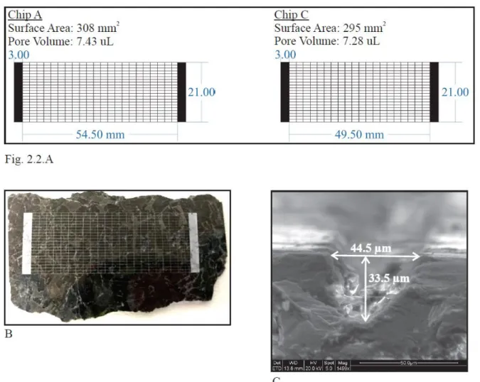
12
The pore network design for one of the microdevices the two microdevices used, (“Chip A”) is a 5.45 x 2.1 cm rectangular grid of comprised of 22 horizontal channels leading from the in port to the out port and 21 vertical channels running perpendicular (Figure 2.2). The pore network for the second chip (“Chip C”) is a 4.95 x 2.1 grid comprised of 22 horizontal channels and 19 vertical channels. Details on pore channel and reservoir measurements using the ESEM may be found in Chapter 3. To accommodate the size of these networks, 2.8 x 7.0 x 0.3 cm wafers were cut and polished as described in Chapter 2.
The microfluidic pore channels are etched into the surface of the polished mineral sample using femtosecond laser plasma mediated ablation with a Yb:CaF2 based, 200fs, chirped pulse amplification laser (Squier et al., 2014) under the ablation conditions reported in Table 2.1.
Table 2.1: Laser ablation conditions of the Yb:CaF2 based laser. laser power (mW) pulse energy (µJ) energy fluence (J cm-2) scanning speed (mm s-1) scan passes lateral spacing (µm) 200 20 17.85 5 6 5
Pore channel designs are first created in CorelDRAW Graphics Suite 2018 and then transferred to G-code and executed semi-automatically with Aerotech machining X-Y and Z stages to achieve the stage conditions recorded in Table 2.2. Pore network designs and general channel dimensions are shown in Figure 2.2.
Laser induced heat affected zones (HAZ’s) are not uncommon in ablation-based material machining (Banks et al., 2000; Sugioka and Cheng, 2014) and are attributed to buildup of plasma pressure and mechanical loading during ablation (Luft et al., 1996). This phenomena is exhibited in various laser ablation techniques including CO2, Nd:YAG pulsed laser, copper vapor laser
13
Table 2.2: Capabilities of the Aerotech Nanopositioning stages used during anorthite channel laser ablation.
series resolution (nm) repeatability (nm) accuracy (nm) in-position stability (nm) maximum speed (mm s-1) ANT130XY 1 75 250 <1 350 ANT130LZS 2 75 300 <2 200
and titanium:sapphire laser ablation and exhibited on a spectrum of materials such as carbon fiber reinforced polymers (CFRP), polyether ether ketone (PEEK) and metallic substrates (Al, Cu, and steel) (Cheng et al., 1998; Pan and Hocheng, 1998; Abedin and Kalla, 2010; Luft et al., 1996). Development of HAZs can be mitigated by cooling the sample with liquid nitrogen (Abedin and Kalla, 2010) and water assisted ablation (Bao et al., 2016; Kruusing, 2004),
optimizing laser scan orientation (Pan and Hocheng, 1998), and adjusting laser flux and induced plasma pressure (O’Keefe et al., 1973; Devaux et al., 1993). An effective approach to limit the development of HAZs is to use an ultrafast pulsed laser such as a pico- (10-12 s) or a femto- (10-15 s) second pulsed laser (Harilal et al., 2014; Luft et al., 1996; Perry et al., 2002; Sugioka and Cheng, 2014). The rapid and precise energy deposition and material removal made possible using ultra-fast laser pulses (compared to continuous laser sources) provide little time for energy transfer into the bulk material (Banks et al., 2000). The extent of heat diffusion into material surrounding the ablating region is minimized, resulting in a relatively undisturbed crystalline lattice and improved nanoscale resolution (Sugioka and Cheng, 2014).
Although the use of the Yb:CaF2 femtosecond laser greatly reduces the extent of HAZ’s, surface modification of the anorthite used for these microdevices is still observed through
14
electron microscopy and Raman spectroscopy. The amorphous mineral phases present in the HAZs are more thermodynamically unstable than crystalline form, resulting in faster dissolution rates (Drever, 1997). Therefore, the HAZ found in our samples was removed prior to flow-through experiments. The HAZ is dissolved from the surface in a hydrofluoric acid solution (0.05% HF buffered by 2.0 % NH4F) for a minimum of three hours. Removal of the HAZ in our samples is verified with electron microscopy and Raman spectroscopy.
In order to characterize and ensure the heat affected layer is completely removed,
transmission electron microscopy (TEM) is used. TEM samples are first prepared to a 100 nm thick lift-out specimen using a gallium sourced FEI Helios Nanolab 600i dual focused ion beam (FIB) with an Omniprobe AutoprobeTM 200 Nano-manipulator and Everhart-Thornley detector. Specimen are then analyzed with the TEM (FEI Talos F200X CTEM/STEM with a Schottky Field Emission Gun) to determine the HAZ thickness before and after HF etching. TEM analyses are completed at 200 kV accelerating voltage and in high angle annular dark field (HAADF), bright field (BF), and dark field (DF) modes. To characterize the extent of the amorphous HAZ, integrated energy dispersive X-ray spectroscopy (EDS - EDAX "Octane Super" silicon drift detector) applied during the STEM analyses is coupled with four silicon drift detectors to map the chemistry of the HAZ and underlying anorthite with up to 0.16 nm resolution.
The extent to which a mineral is crystalline or amorphous has been shown to impact it’s characteristic Raman spectra due to the absence of structural order and symmetry within an amorphous material (Murata et al., 2009; Pop et al., 2015; Tushcel, 2017). Spectra of amorphous materials tend to have broader, shorter peaks, while crystalline material exhibit higher, more well-defined peaks. These identifiers make Raman spectroscopy a useful tool to validate whether the heat affected zone is fully removed prior to sealing the microdevices. A WITec alpha300R
15
confocal Raman Microscope is used for detecting the presence of the heat affected zone. Images taken with the Andor DV401A-BV-352 CCD camera and spectra are produced using the Ultra High Throughput Spectrometer (UHTS) with a 600 groove/mm, 500 nm Blaze Wavelength echelette grating. The excitation laser wavelength is 532 nm with a 599 nm spectral center. Measurements are taken using a light shield and UHL KT5 NOOA motorized sample stage while spectra are generated using single second integration times, ten spectral accumulations and -60˚C operating condition. WITec Control version 1.52 software is used to process images and spectra. 2.4 Sealing the Pore Network
Clear Dow Corning Sylgard 184 Encapsulant is mixed in an 8:1 base to agent ratio for 5 minutes in 10 cm diameter petri dishes. A glass slide is cut to the size of the pore network and placed in the bottom of the PDMS during curing to produce a ~1mm thick, optically transparent section to cover the pore network with thicker (3-5 mm) sections at both ends to provide stability for the capillary tubing which is inserted into holes punched into the PDMS (Figure 1E and 3B). The mixture is placed in a vacuumed desiccator for at least 15-20 minutes, then cured on an 80˚C hot plate for four hours. Holes are punched in the thicker PDMS at the location of each reservoir using biopsy punches from World Precision Instruments (0.75 mm diameter). Following ablation and removal of the HAZ, samples and PDMS covers are cleaned in sonicated baths of acetone, ethanol and then deionized water for five minutes each and oven dried at 80˚C for an hour. Next, a Harrick Plasma Inc. plasma cleaner is used to vacuum, oxygen flush, and plasma bond the PDMS to the mineral surface. The bonding quality is increased by heating samples at 80˚C overnight.
2.5 Solution Preparation, Injection, and Collection
16
0.001 M sodium chloride (NaCl) added to increase the conductivity and stabilize pH readings. One stock solution is acidified to approximately 1 M HCl, and both stock solutions are combined to create flow through solutions of pH’s ranging from (~ 3.0 to ~5.0). pH of the stock solutions are measured with a micro pH probe (Thermo Orion PerpHeT Ross combination pH Micro Electrode, 8220BNWP) and with Ultra pH/ATC probes (Thermo Orion 8107UWMMD). pH measurements are taken with both probe types prior to syringe filling and 500 μL effluent samples are measured with only the PerpHet microprobe upon collection. Three point
calibrations are done with each probe before every use. If calibrations are below 94%, buffers are refreshed, and a new calibration is taken.
Tests are conducted with a Cole Parmer Dual Independent Touch Screen Syringe Pump (Model GTM96600-6048-18-T3) with injection by a Hamilton 81401 Gastight Syringe with Luer Tip (2.5 mL) and an inert PTFE-coated plunger (Figure 2.3). Solutions are collected in 500 μL autosampler vials and measured with the Orion micro pH probe upon collection. Calcium ion concentrations are measured using a DionexTM ICS-1100 Ion Chromatography System, AS-DV Autosampler, and Chromeleon Chromatography Management System software, and 20 mM MSA eluent. Operating conditions may be found in Appendix A.
2.6 Data Collection and Analysis
Steady state for this system is defined when the flux-time derivative and coefficient of variance curve fall below pre-defined respective thresholds. A four to five hundred pore volume moving average of both curves dampens inherent variations, averaging over approximately 4 sampling events. Effluence Ca2+ concentrations are considered to be at steady state when the derivative is below ±2×10⁻⁹ mg/min and the coefficient is below 0.5 as these thresholds tend to
17
demark a change from overall higher spreads and averages in flux at points in time before steady state to lower after the system has reached steady state.
All processed flux and residence time data is derived from the first one thousand pore volumes which were collected at the beginning of the defined steady state period, and
experimental runs were not considered finished until a minimum of one thousand steady state pore volumes were consistently reached. Uncertainty was applied to average calcium fluxes and dissolution rates using Equation 2.1 where Z is the calculated dissolution rate, and W, X, and Y are the variables used in calculating Z such as the calcium flux, flow rate, and surface area. δ is the uncertainty associated with each value. Sources of uncertainty are described in the
Discussion of Chapter 4. 𝛿𝑍 = 𝑍 × √(𝛿𝑊𝑊) 2 + (𝛿𝑋 𝑋) 2 + (𝛿𝑌 𝑌) 2 (2.1)
18
Figure 2.1 Experimental preparation and procedures include A) cutting and polishing mineral specimen, B) laser ablation of the channel pore network, C) microanalysis of the heat affected zone, D) removal of the heat affected zone, E) sealing of the pore network trough plasma bonding PDMS to the surface, F) running flow through experiments with a dual syringe pump, and G) analysis of influent and effluent using ion chromatography. Note the samples in figures 1A, B, and E were not used for the experiments reported in this work.
19
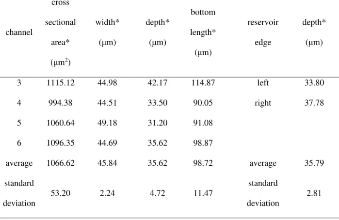
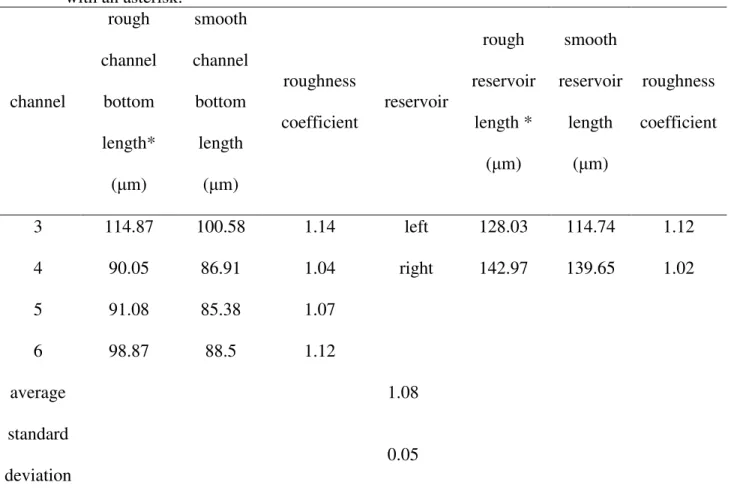
Figure 2.2 A) Dimensions of pore network designs used for both anorthite samples calculated using a roughness coefficient of 1.08. B) A newly ablated sample pattern. C) ESEM image of laser ablated pore channel cross section with approximate width and depth
20
Figure 2.3 Schematic (top) and photos (bottom) of bench top set up. A) The syringes filled with injection fluid are mounted in a syringe pump. B) Flow-through solution enters, reacts with, and exits the microdevices, and C) effluent is collected in autosampler vials for pH and ion chromatography measurements.
21
CHAPTER 3: RESULTS
Microdevice pore networks were characterized for chemistry and morphology to ensure representative specimen and dissolution rates. We analyzed the effects of pH and residence on the dissolution rates within our microdevices as measured by calcium ion content in experiment effluent.
3.1 Anorthite Mineralogy and Grainsize
The majority of the Grass Valley anorthite used for this study are comprised of
predominantly (~90%) anorthite (5-15 mm long grains) with minor amounts (~8%) of pyroxene (up to 6 mm long grains) (Figure 3.1.A). Elevated iron, magnesium and silicon detected with EBSD and Raman spectra (Figure 3.1) indicate trace amounts of an enstatite (MgSiO3) - (~2%) ferrosilite (FeSiO3) series within the samples. Iron and oxygen were detected indicating trace amounts of magnetite (Fe3O4) surrounded by elevated titanium and oxygen which may be trace ilmenite. (FeTiO3), (Figure 3.1.B). These grains are approximately between 100 and 200 μm in length respectively.
3.2 Microfluidic Device Characterization: Channel Chemistry and Crystallinity The first ablated sample used in this study (“Chip A”, Figure 2.2) was analyzed using
scanning transmission electron microscopy (STEM) to assess the extent of ablation induced HAZ and to verify its removal after the HF solution bath. For a more efficient analysis of HAZ extent and removal, subsequent samples are analyzed using Raman spectroscopy.
TEM analyses show a change in anorthite chemistry with greater proximity to the ablated sample surface (as demarked by the platinum applied to the surface to mitigate ion damage during sample preparation in the focused ion beam). Calcium, among other elements including
22
sodium, and aluminum, was depleted within ~500 nm of the surface for a sample etched in the HF solution for 2.5 hours (Figure 3.2.A and B). Silica (shown in Figure 3.2.B) and oxygen were the only elements analyzed which were enriched within 500 nm of the platinum layer. These results indicate that upon laser ablation, elements other than silica and oxygen are being removed at least 500 nm from the mineral surface while silica and oxygen remain, creating a surface unrepresentative of natural anorthite. In addition, the TEM analyses indicate this ~500 nm HAZ still remains in the ablated anorthite despite 2.5 hours of HF etching. Therefore, samples must be submerged in the HF solution for more than 2.5 hours for the HAZ to be fully removed. of calcium, silica, sodium, aluminum, and oxygen remain relatively constant until reaching the platinum, where they uniformly deplete, indicating a sharp boundary between the anorthite mineral and the platinum layer, meaning that the HAZ was fully removed from the anorthite surface.
Chip A was submerged for an additional 2.5 hours resulting in 5 hours of HF bathing in total. After the additional HF bath, the HAZ was entirely removed as shown in TEM analyses (Figures 5C and D). The abundance
Diffraction patterns of both the 2.5 and 5 hour etched samples were taken within several nanometers of the platinum layer. The 5-hour etch presented a clear diffraction pattern indicating that the crystallography of the anorthite is preserved and that the HAZ is fully removed (Figure 3.2.E). Although the 2.5 hour etch presented a diffraction pattern, the line scan served as chemical evidence that the HAZ still remained.
The combined line scans and diffraction analyses effectively show that the HAZ is removed upon HF acid baths lasting between 2.5 and 5 hours, exposing both the natural chemical and crystalline structure of the anorthite (Figure 3.2). Additionally, these TEM/STEM and EDS
23
observations indicate that the HF etching procedure does not compromise the crystallinity or chemistry of the anorthite surface initially below the HAZ.
Raman spectra (Figure 3.3.A) were taken of non-ablated, polished anorthite surfaces (Figure 3.3.B), and ablated anorthite regions which underwent 0 (no HF bath), 2, 2.5, and 3 hours of the HF bathing procedure described in Chapter 2. The series of spectra include signatures of the ring-breathing vibrational mode of the silica-tetrahedra in all samples as indicated by the doublet at 490 and 520 cm-1 (Freeman et al., 2008; Wang et al., 1995, 1994). In this mode, the
assemblage expands and contracts through the tetrahedra-oxygen bonds. Additionally, the rotation-translation mode signature is present in the polished and HF bathed samples (290 cm-1). The signature of the polished sample includes all aforementioned peaks in addition to
deformation mode peaks (770 and 800 cm-1). The 680 cm-1 may be related to the Si-O-Si bonding mode observed in high enstatite (0.7-0.975), low ferrosilite (0.02- 0.2) orthopyroxenes (Sharma et al., 1983; Huang et al., 2000). In general, peak signatures are often obscured in Raman spectra by accompanying silicates and salts (Freeman et al 2008) and may be a
reasonable indication that HAZ is still present. The accumulation of silica and oxygen shown in the TEM linescans of the 2.5 hour etched sample may potentially be responsible for obscuring peak signatures of the anorthite below the HAZ.
Reflective light microscopy documents a smooth surface for the polished mineral, an undistinguishable, white surface for the ablated, non-HF bathed sample, and more distinguishable, granular surfaces for the ablated then HF bathed samples.
3.3 Channel Morphology: Geometry and Roughness
Depths, widths, and roughness coefficients (effective length (Le) /length (L)) of ablated features in the microdevices were measured using scanning electron micrographs of channel and
24
reservoir cross sections and the drawing program InkScape 0.92.2. Four channels and the left and right edges of a single reservoir were analyzed to determine an average channel cross sectional area of 1066 μm2 and an average roughness coefficient of 1.08 ± 0.05 (Figure 3.4, Tables 3.1A and 3B). We applied the roughness coefficient to channel cross sectional surface areas and to reservoir as well as channel depths, widths and lengths. With these dimensions, we determined that Chip A has a surface area of 308 mm2 and a pore volume of 7.43 μL while Chip C has a surface area of 295 mm2 and pore volume of 7.28 μL. Pore volumes include both fluid reservoirs at the in and out port (Figure 2.2.B). Calcium ion fluxes and dissolution rates were calculated using the pore volumes and surface areas derived from the measurements presented here (Tables 3.1 and 3.2).
Table 3.1: Measurements of channel and reservoir cross sections dimensions. Measurements taken from rough, not smooth outlines are indicated with an asterisk. channel cross sectional area* (μm2) width* (μm) depth* (μm) bottom length* (μm) reservoir edge depth* (μm) 3 1115.12 44.98 42.17 114.87 left 33.80 4 994.38 44.51 33.50 90.05 right 37.78 5 1060.64 49.18 31.20 91.08 6 1096.35 44.69 35.62 98.87 average 1066.62 45.84 35.62 98.72 average 35.79 standard deviation 53.20 2.24 4.72 11.47 standard deviation 2.81
25
Table 3.2: Measurements of channel and reservoir cross sections roughness coefficients. Measurements taken from rough, not smooth outlines are indicated with an asterisk.
3.4 Effluent Chemistry and Reaction Rates
Appendix B contains plotted and tabulated flux and rate data (Table B2, Figures B.1 and B.2). Mean calcium flux detected from the effluent ranged from 7.34×10⁻⁸ mg min-1 in the pH 5, 0.5 μL min-1 test to 6.44×10⁻⁷ mg min-1 measured from the pH 3, 2 μL min-1 test (Table 3.3). Mean dissolution rates range from 9.91×10⁻¹⁰ to 8.83×10⁻⁹ mol m-2 sec-1 again, as measured from the pH 5, 0.5 μL min-1 and pH 4, 2 μL min-1 tests, respectively.
3.4.1 Dissolution Rates and pH within Our Microdevices
Figure 3.5 presents the calculated dissolution rate data as a function of pH and residence time (τ). In general, the 2 μL min-1 flow rate tests result in the greatest dissolution for each pH. channel rough channel bottom length* (μm) smooth channel bottom length (μm) roughness coefficient reservoir rough reservoir length * (μm) smooth reservoir length (μm) roughness coefficient 3 114.87 100.58 1.14 left 128.03 114.74 1.12 4 90.05 86.91 1.04 right 142.97 139.65 1.02 5 91.08 85.38 1.07 6 98.87 88.5 1.12 average 1.08 standard deviation 0.05
26
Table 3.3: Pore volume, pH, calcium flux, and dissolution rate data for each of the nine experiments. Results of each test are summarized here.
The lowest rates for the pH 3 and 4 tests were produced from the 1 μL/min tests and for the pH 5 tests were generated from the 0.5 μL min-1 flow rate test. When considering the rates at each pH averaged across the three flows (first and second columns in Table 3.4), the mean dissolution rate concluded from all pH 3 tests is 7.11×10⁻⁹ mol m-2 sec-1, while the pH 4 average is less at 5.50×10⁻⁹ mol m-2 sec-1 and the pH 5 average the lowest at 1.89×10⁻¹⁰ mol m-2 sec-1, creating in general, an expected inverse correlation between pH and dissolution rates among the data within these tests. This generalized correlation is not as strong for individualized cases at each flow rate
Flow Rate (μL min-1) Average Influent pH Residence Time (τ, min) Average Ca2+ Flux (mg min-1) Total Ca2+ Flux Error (mg min-1) Average Dissolution Rate (mol m-2 sec-1) Total Dissolution Rate error (mol m-2 sec -1) 2.25 3.07 3.30 6.44×10⁻⁷ 3.9×10⁻⁸ 8.70×10⁻⁹ 6.7×10⁻¹⁰ 2.25 4.08 3.24 6.26×10⁻⁷ 3.8×10⁻⁸ 8.83×10⁻⁹ 6.9×10⁻¹⁰ 2.25 5.17 3.24 2.13×10⁻⁷ 1.3×10⁻⁸ 3.01×10⁻⁹ 2.3×10⁻¹⁰ 1.13 3.08 6.44 3.69×10⁻⁷ 2.3×10⁻⁸ 5.21×10⁻⁹ 4.0×10⁻¹⁰ 1.13 3.99 6.44 3.69×10⁻⁷ 2.3×10⁻⁸ 1.53×10⁻⁹ 1.2×10⁻¹⁰ 1.13 4.98 6.58 1.24×10⁻⁷ 7.5×10⁻⁹ 1.67×10⁻⁹ 1.3×10⁻¹⁰ 0.56 3.07 13.27 5.49×10⁻⁷ 3.3×10⁻⁸ 7.41×10⁻⁹ 5.7×10⁻¹⁰ 0.56 4.12 13.00 4.35×10⁻⁷ 2.7×10⁻⁸ 6.13×10⁻⁹ 4.8×10⁻¹⁰ 0.56 5.08 13.27 7.34×10⁻⁸ 4.5×10⁻⁹ 9.91×10⁻¹⁰ 7.7×10⁻¹¹
27
however (third through fifth column of Table 3.4). In Figure 3.5.B, we see that for the fastest flow rate at 2 μL min-1 (~3 minute τ) and the slowest flow rate at 0.5 μL min-1 (~13 minute τ), there is very little variation between the pH 3 and pH 4 data, while the pH 5 residence time is, as expected, the lowest among the three in both cases. For the intermediate, 1 μL min-1, flow rate, (~6 minute τ) while the pH 3 dissolution rate is the greatest, there is little difference between the pH 4 and 5 dissolution rates, and unexpectedly, the pH 4 dissolution rate is the lowest of all three. A discussion regarding potential causes of the unforeseen trend in pH and τ at the 1 μL min-1 flow rate is presented in the Discussion.
Table 3.4: Dissolution rates for each pH averaged across all three flow rates and rates for each flow rate averaged across all three pH’s.
pH Average Dissolution Rate of all three flow
rates (mol m-2 sec-1)
μL min-1 Average Residence Times (τ, min) Average Dissolution Rate of all three pH's (mol m-2 sec-1) 3.07 7.11×10⁻⁹ 2.25 3.25 6.85×10⁻⁹ 4.06 5.50×10⁻⁹ 1.13 6.49 2.80×10⁻⁹ 5.08 1.89×10⁻⁹ 0.56 13.18 4.84×10⁻⁹
3.4.2 Dissolution Rates and Residence Times within Our Microdevices
Rates averaged by residence time (τ) do not follow an inverse correlation, however. The average dissolution rate of ~3 minute τ tests is the greatest 6.85×10⁻⁹ mol m-2 sec-1, the average rates of ~6 minute τ tests is the lowest 2.80×10⁻⁹ mol m-2 sec-1 while the ~12 minute τ tests lie in the middle at 4.84×10⁻⁹ mol m-2 sec-1 (Figure 3.5.B, Table 3.3). Dissolution rates considered at
28
pH 3 and 4 reveal a similar trend. At pH 3, the lowest τ test produces some of the greatest dissolution rates, while the intermediate τ results in the least dissolution. The difference between each dissolution rate at pH 3 is minimal to insignificant, however, upon considering error. The pH 4 test shows the same trend between τ and dissolution rates, yet the difference between the intermediate τ is significant, placing the pH 4, ~6 min τ rate (1.53×10⁻⁹ mol m-2 sec-1) within the range of the pH 5, ~6 minute τ data (1.67 ×10⁻⁹ mol m-2 sec-1). At pH 5, the correlation between dissolution rate and τ is inverse with the lower τ data having minimal spread, and the higher τ data being significantly lower. A discussion regarding potential sources of the unforeseen trends in the pH 3 and 4 data is presented in the Discussion.
29
Figure 3.1 ESEM characterization of Grass Valley anorthite hand sample. A and inset) Within the anorthite (”an”) exist a grain of ferrosilite (”ferr”) and a magnesium rich pyroxene (”opx”), potentially enstatite. Peaks indicative of enstatite in these samples are also documented in Raman spectra. B) An iron oxide impurity in anorthite matrix is suspected to be a magnetite (”mag”) grain accompanied by ilmenite (”ilm”).
30
Figure 3.2 Analysis of ablated anorthite reservoir after a 2.5 hour (A and B) and a 5 hour (C through F) HF bath to remove amorphous HAZ. STEM line scans (5B and D) show the composition along the anorthite (”an”) - platinum (”pt”) interface. Although sodium, aluminum, and oxygen are not shown, they exhibit a similar profile to calcium. Line scan data accounts for spectra compiled from the entire dashed outlined regions. E) The diffraction pattern taken of the 5 hour HF etch (ROI within several nm of the platinum)
indicates that the crystal structure is preserved, and therefore the HAZ is removed.
31
Figure 3.3 Raman spectra of incremental HF etching (A). Reflective light images of analyses locations for each spectra (B through F). All images were taken at 20X magnification.
32
Figure 3.4 An example of channel and reservoir cross section measurements as presented in Table 3. The network pore volume was calculated using the channel cross sectional areas (shaded green), the effective lengths of the reservoir bottoms, and the depths of the reservoir bottoms (dashed). Pore network surface areas were calculated using the effective lengths of the channel and reservoir bottoms (yellow). Effective lengths (yellow) and generalized lengths (red) were used to calculate roughness coefficients of the pore network. Measurements were made using the ESEM and the drawing program, Inkscape 0.92.2.
33
Figure 3.5 Variations in dissolution rates with tested pH’s (A), and tested flow rates (B) for the tests executed with our microdevices. Residence times near 3 minutes correspond to the 2 μL/min flow rate tests, while residence times near 6.5 minutes correspond to 1 μL/min tests and ~13 minute residence times to 0.5 μL/min tests.
34
CHAPTER 4: DISCUSSION
Our dissolution rates were put in context with others measured under a range of pH’s and residence times. We explore reasons for unexpected dissolution rate results and propose ways to constrain experimental uncertainties for future tests.
4.1 Plagioclase dissolution measured with different approaches at different scales The anorthite dissolution rates measured in this study’s microdevices are within the range of previously reported rates that were measured at pH’s 1.5- 6 (5.2×10⁻¹⁴ to 2.5×10⁻⁷ moles m-2 sec-1 in other literature) (Figure 4.1). Within this range, our results exist among faster rates (~1×10⁻⁹ moles m-2 sec1) which are derived from studies also involving laboratory conducted experiments using well-mixed solutions and relatively homogenous samples (Table 4.1, Fleer, 1982;
Gudbrandsson et al., 2014; Casey et al., 1991; Carroll and Knauss, 2005). As was done for our tests, all laboratory experiments with the exception of Carroll and Knauss, 2005 were also conducted under ambient pressure and temperature conditions. Additionally, the flow through solutions in these low pH, high dissolution rate studies were acidified with HCl and often ionized with NaCl similar to our approach.
Within this range of rates and pH’s, our dissolution rates are among the highest with the exception of those reported in Fleer, 1982. While other laboratory dissolution rate studies used powdered plagioclase samples in batch reactors or columns, Fleer, 1982 used polished (1 μm grit) single anorthite crystals, and our microdevices employ dissolution of an ablated mineral surface. This implies that regardless of pH, the study scale (batch and column versus specifically microdevice) may also influence dissolution rates. This influence is seen among other studies, specifically in the field and laboratory experiments of Swoboda-Colberg and Drever, 1993. Both
35
lab and field experiments were conducted with solutions of pH 4 and 4.5, and yet rate
discrepancies existed across multiple orders of magnitudes (laboratory rates of 2.38 to 2.36×10⁻¹¹ moles m-2 sec-1 and field rates of 1.46×10⁻¹³ and 5.2×10⁻¹⁴ moles m-2 sec-1). Reasons for the discrepancies between field vs laboratory and batch, column vs. microdevice are addressed in Chapter 4.
Table 4.1: Supplemental experimental information on literature included in Figure 4.1.
Source Laboratory/Field Dissolution Environment Plagioclase Material Plagioclase Grain Size, if applicable SSA, if applicable (m2g-1) § surface area (m-2) this study Laboratory Microfluidic Single
crystal
n/a § 2.6-2.7×10⁻⁴
Fleer, 1982 Laboratory Batch Single crystal
250-500 μm 0.08 -0.107
Holdren and Speyer, 1987
Laboratory Batch Powder 30->400 μm 0.483-4.475
Casey et al., 1991
Laboratory Batch Powder 25-75 μm 0.18-0.645
Amrhein and Suarez, 1992
Laboratory Batch Powder 20-50, 50-100, 100-250 μm
0.5, 0.3, 0.11
36 4.2 Implications of the Impact of Residence Time
An inverse correlation between dissolution rates and residence times (τ ) ranging from 1×10⁻³ years to 105 years has been well established in past literature (Figure 4.2, Berne, 1978, Wolock, 1997, Maher, 2009, Maher 2010, Jung and Navarre-Sitchler, 2018). With the exception of Lüttge and Bolton's, 1999 scanning interferometry study, plagioclase dissolution rates achieved under τ
Table 4.1 Continued Gudbrandsson
et al., 2014
Laboratory Batch Powder 45-125 μm 0.0944
White et al., 2017
Laboratory Column Crushed granules
0.25 – 0.85 mm
0.63-1.97
Zhu, 2005 Field Batch Sand
particles
0.1-0.2 mm 2.85
Daval et al., 2018
Laboratory Batch Powder n/a 0.51
Carroll and Knauss, 2005
Laboratory Batch Powder 150-240 μm 0.03
Swoboda-Colberg and Drever, 1993
Laboratory Batch Powder 75-150 μm 0.02
Swoboda-Colberg and Drever, 1993
Field Plot Scale Original particles
< 2 μm – 2 mm
37
as low as ours – on the order of minutes – have not yet been reported to our knowledge. Because of this, our experiments extend the limits of this established relationship to τ an order of
magnitude lower than previously identified (Figure 4.2).
Of the studies presented here, Burch et al., 1993 reports plagioclase dissolution rates that are most similar to ours, despite the fact that their experiments differ from ours in that they conducted tests under elevated temperatures (80˚ C), with pH 8.8 solution, and studied crushed albite dissolution in continuously-stirred flow through reactors. Despite these differences between our experiments, the Burch et al., 1993 study had similar residence times (5- 67 hours) and (Figure 4.2) and ultimately the similar reaction rates. The studies presented in Figure 4.2 with dissolution rates least like ours – the lowest rates in the range of 1×10-16 and 3.5×10⁻¹⁷ moles m-2 sec-1 are those of Maher et al., 2006 and Zhu, 2005. Both studies are similar to one another in that they both considered field scale dissolution rates and reported τ ranging from 10k to 37k years. A variety of field and laboratory (colored triangles) cases are plotted between ours and those of Maher et al., 2006 and Zhu, 2005. Despite variations in parent material, sample grain size, reaction temperature, and surface area, the inverse relationship is robust across orders of magnitudes in reaction rates and τ (Table 4.2, Figure 4.2). Suspected reasons for this
prevailing trend are described.
Regardless of the setting, dissolution reactions will progress towards dynamic equilibrium, a state of maximum thermodynamic stability (IAP/Keq ~1). Initially, effective dissolution reaction rates may begin high, because solutions are under low, far from equilibrium conditions where IAP/Keq (~<0.1). As the fluid travels through a system and becomes more saturated with dissolution products, the system approaches equilibrium conditions and is closer to being saturation-state-limited. Therefore, with increased τ – induced by a number of factors including
38
Table 4.2: Supplemental experimental information on literature included in Figure 4.2.
Source Laboratory/Field Dissolution Environment Plagioclase Material Plagioclase Grain Size, if applicable SSA, if applicable (m2g-1) § surface area (m2) Burch et al., 1993 Laboratory Bed-Flow Reactor Powder <20 μm, <43 μm 0.65-0.83 Clow and Drever, 1996 Field 39 m2 Catchment Sand >0 μm to 2 mm *0.05 - 9.27
Jin et al., 2008 Field
Deep Soil Profile Clay and Sand **0.004- 2 mm not reported Kim, 2002 Field Silicate Aquifer Sand 0.1-0.5 mm .011-.029 Maher et al., 2006 Field Deep Sea Sediments Clay 8-3 μm 1.3- 3.2 Swoboda-Colberg and Drever, 1993
Laboratory Batch Powder 75-150 μm 0.02
Swoboda-Colberg and Drever, 1993 Field 2 m2 Spodosol Plot Original particles < 2 μm – 2 mm § 24,511
39 White et al., 2017 Laboratory Column Crushed granules 0.25 – 0.85 mm 0.63-1.97
Zhu, 2005 Field Batch
Sand particles
0.1-0.2 mm 2.85
*from variety of minerals with no specific data on plagioclase
** specific grainsizes not reported, so value is derived from Wentworth, 1922 Table 4.2 Continued
White and Brantley, 2003
Laboratory Column Powder < 2 mm .084 - 5.33
White and Brantley, 2003
Laboratory Column Powder < 2 mm .084 - 5.33
White et al., 2001 Field Regolith (Bedrock Saprolite, Soil) Crystalline > 1 mm 1 White et al., 2005 Field 100 m2 Riverbank Plot Granitic Sand **0.125 - 1 mm 0.45-1.48 White et al., 2008 Field Augered, Marine Terrace Sandstone **0.125 - 1 mm 1.94E+00
40
dissolution rates decrease in near-equilibrium systems (Jung and Navarre-Sitchler, 2018a). Figure 4.2 conveys that this process is prevalent despite a variety of source materials, temperatures, grain sizes, and results in τ ranging from minutes to thousands of years. In
particular, when expanding from our microfluidic device to column to field scale, more complex geologic settings inherently have wider distributions of flow paths and flow rates. This results in zones of greater τ and thus lower dissolution rates, offering one explanation for the discrepancies in plagioclase dissolution rates among laboratory experiments and between lab and field reaction rates.
4.3 Trends in Dissolution Rates within Our Microdevices
The correlation between pH and dissolution rates was expected to be inverse regardless of residence time (τ). The ~3 and ~13 minute τ data align with this trend relatively well with little variation between the pH 3 and 4 rates and significant decreases in the pH 5 dissolution rates (Figure 3.5). However, the ~6 minute τ data diverges from this relationship, with the greatest deviation among the pH 4 data. This leads us to suspect that the pH 4 test result is anomalously low.
Additionally, the correlation between residence times and dissolution rates was also expected to be inverse regardless of pH. The pH 5 data follows this trend, despite over lapping error for the ~3 and ~6 minute τ rates. The pH 3 dissolution rates are very similar at the ~3 and ~13 minute τ, with minimal difference between these rates and that of the ~6 minute τ test. These results indicate that within our systems, τ has little effect on dissolution rates with pH 3 influent. The pH 4 dissolution rates at ~ 3 and ~13 minute τ are also similar to one another while the ~ 6 minute τ test resulted in a significantly lower dissolution rate. This would indicate that within our
41
system, τ impacts the pH 4 dissolution, but not according to the inverse relationship we had expected. Again, the pH 4, ~6 minutes τ test is suspected to be an outlier within this system.
The microdevice (Chip A or C) used for each test, the correlation of test dates, background calcium in the Milli-Q water used to make the chromatography eluent, and the occurrence of microdevice leaks or influent pH alterations were investigated to determine a cause of the substantially low pH 4, ~6 minute τ data (Appendix C). Several observations can be made from this review, and the ultimate conjecture is to repeat the pH 4, ~6 minute τ test.
First, there does not appear to be a distinct correlation between microdevice (A or C) and dissolution rate (Table C.1). The lower dissolution rates resulted from the pH 3 and pH 4 tests at ~6 minute τ both ran on Chip C. However, pH 3 and pH 4 tests ran using both microdevices A and C exhibited greater rates during the ~3 and ~13 minute τ tests, indicating that both low and higher dissolution rates are possible from either chip. The pH 5 test dissolution rates remained consistently lower despite running on chip C for ~3 τ, and Chip A for the ~6 and ~13 τ, implying that similar rates are produced from both chips at a similar pH.Secondly, tests with similar dissolution rates were ran in conjunction with one another. For example, the pH 3, 4 at ~3 minute τ tests have similar dissolution rates and were ran side by side (Table C.1). The same is true for pH 3, 4 at ~13 minute τ tests and the pH 4,5 at ~6 minute τ tests. Yet this observation does not explain the underlying mechanism for the lower rates at ~6 minute τ, particularly for the pH 4 test.
Potential IC effluent contamination was also a potential factor, and the calcium in the Milli-Q water blanks were correlated to each test (Table C.1). The third observation is that there is no strong correlation between lower dissolution rates (such as that for the pH 4, ~6 minute τ test) and calcium concentration in the background Milli-Q water. For example, the higher dissolution