Analytic hierarchy process approach to determination of combat power, The

THE ANALYTIC HIERARCHY PROCESS APPROACH TO DETERMINATION OF COMBAT POWER

by

All rights reserved INFORMATION TO ALL USERS

The qu ality of this repro d u ctio n is d e p e n d e n t upon the q u ality of the copy subm itted. In the unlikely e v e n t that the a u th o r did not send a c o m p le te m anuscript and there are missing pages, these will be note d . Also, if m aterial had to be rem oved,

a n o te will in d ica te the deletion.

uest

ProQuest 10783705

Published by ProQuest LLC(2018). C op yrig ht of the Dissertation is held by the Author. All rights reserved.

This work is protected against unauthorized copying under Title 17, United States C o d e M icroform Edition © ProQuest LLC.

ProQuest LLC.

789 East Eisenhower Parkway P.O. Box 1346

A thesis submitted to the Faculty and the Board of Trustees of the Colorado School of Mines in partial

fulfillment of the requirements for the degree of Master of Science (Mathematics) Golden, Colorado Date Signed Approve D r . R u t h A. Ma&rer Thesis Advisor Golden, Colorado Dr. Ardel J. Boes Professor and Head Mathematics Department

ABSTRACT

The problem in this thesis is based on the military description of combat power. The military definition of combat power as defined by the military is a complex combination of tangible and intangible factors which are transitory and reversible on the battlefield. The intangible factors that are in combat power make it a very subjective evaluation. In current military doctrine the problem of how to deal with the intangible factors is never discussed. In this thesis the intangibles are not only considered but are used in calculating combat power using the Analytic

Hierarchy Process (AHP) developed by Thomas L. Saaty in the late 70's.

The AHP is able to take complex problems and break them down into a hierarchy of criteria and alternatives. Once the hierarchy is established a pairwise comparison between the alternatives and criteria is performed to calculate the priorities for the alternatives. In calculating combat

power, companies and avenues of approach can be compared against one another using both tangible and intangible criteria to rank order the alternatives.

This thesis was able to define what combat power is using a precise mathematical model, It illustrates how both tangible and intangible factors are used to compute combat power.

. TABLE OF CONTENTS Rage ABSTRACT iii LIST OF FIGURES v ACKNOWLEDGMENT S vi i CHAPTER 1. LITERATURE REVIEW 1 1.1 Military Research 3 1.2 Mathematical Research 5

1.2.1 Calculating Combat Power 6 1.2.2 Assigning Combat Power 9 2. ANALYTIC HIERARCHY APPROACH 11

2.1 Introduction To AHP 11

2.2 Analytic Hierarchy Process 13

2.3 AHP Scale 25

2.4 Consistency 28

2.5 Group Interaction 32

2.6 Justification of the Method 35

3. MILITARY APPLICATION 43

3.1 Command Estimate 45

3.2 Combat Power 46

3.3 Combat Criteria 47

3.4 Analytic Hierarchy Process 48 3.5 Quick and Dirty Combat Power 55

3.6 Combat Power Worksheet 57

3.7 Enemy Avenues of Approach 60 3.8 Assignment of Combat Power 62 3.9 Reasoning Behind Reserve 67

3.10 The Basic Algorithm 69

3.11 Example of Assignment Problem 71

3.12 Sensitivity 77

4, CONCLUSION 90

4.1 Summary 90

4.2 Recommendations for Further Research 92

REFERENCES CITED 95

14 15 17 19 20 21 22 24 26 27 30 49 50 52 54 58 60 62 64 65 66 68 72 GPA Two Level Hierarchy

Pairwise Comparison Scale GPA Judgmental Matrix

Computed GPA Judgement Matrix GPA Three Level Hierarchy Three Level Computed Pi

Three Level Judgement Matrices Three Level Composite Priorities Scale Example

Actual Scale Comparison Random Consistency Index Combat Power Hierarchy

Combat Power Comparison of Criteria Combat Power Criteria Matrices

Focus Combat Power Comparison Table

Combat Power Worksheet

Assignment Hierarchy Structure Assignment Criteria

Assignment Criteria Judgement Matrices Focus of Combat Power

Reserve Step One

75 76 77 79 80 81 82 83 84 85 86 87 88 Step Four Battlefield Layout

Battlefield Layout With Reserve Gradient Equipment Sensitivity Dynamic Equipment Sensitivity Gradient Tank Gunnery Sensitivity Dynamic Tank Gunnery Sensitivity

Gradient Engineer Support Sensitivity Dynamic Engineer Support Sensitivity Gradient Crew Strength Sensitivity Dynamic Crew Strength Sensitivity Gradient Firing Mode Sensitivity Dynamic Firing Mode Sensitivity

Acknowledgments

First I would like to thank my wife Linda for all the support she has given me through this endeavor. Without her love and belief in me this thesis would not have been

possible.

I thank Dr. Ruth Maurer for not only being my thesis advisor but also for being a leader and mentor. Dr.

Maurer's guidance and experience in this project has been irreplaceable. I will use the knowledge and experience she has given me throughout my military career,

I would like to express my sincere appreciation for the advice and assistance given by my committee members Dr. R.E.D. Woosley and Ltc. Bruce Geotz. Thanks to all my

colleagues in the guild, especially Mark Gulley, for all the help and advice they gave me.

Lastly and mostly, I thank my mother Louise Barton for always being there when I needed her. Through her

dedication and love she has gotten me where I am today.

Chapter One Literature Review

Military commanders have used combat power for centuries to analyze a course of action to take on the battlefield. As early as 500 B.C. Sun Tzu wrote of combat power as the energy needed to defeat the enemy in his book

The ART of W A R . The current definition of combat power as

defined in FM 101-5-1 Operational Terms and Symbols is

A complex combination of tangible and intangible factors which are transitory and reversible on the battlefield. Combat power is comprised of the effects of maneuver, the effects of firepower, the effects of protection, and the effects of leadership. The

skillful combination of these elements in a sound operational plan will turn potential into actual power.

To adequately compare different alternatives, they must be analyzed by using the same criteria. These criteria should be carefully selected, since they may greatly effect the outcome of the problem. Both the tangible and

intangible criteria can change the results of an analysis; therefore, both should be included in the decision making

process. If the criteria are poorly selected, the solution to the problem maybe incomplete and the analysis

inadequate.

An embedded problem in using combat power for

analyzing courses of action is that there is no current US military doctrine explaining how to calculate a

quantitative value for comparing units. ST 100-9 The

Command Estimate explains what to do with a unit's combat power but fails to define how to determine it. The manual uses notional values for instructional purposes and fails to determine combat power because of the complex tangible and intangible factors that make up a unit's combat power. There are many tools in the mathematical world that can assist the military commander in calculating and assigning combat power. In the world of decision making there are numerous processes that can deal with multi-criteria

analysis. Chapter one will deal with some of the different processes the military commander may use to determine

combat power and how the commander can assign this combat power. The second problem deals with the assigning of the combat power to enemy Avenues of Approach. Since there are numerous different ways of assigning combat power,

commanders must first decide what their goal is for the assignment of units. Once the goal has been decided the

method of assignment can be chosen. As in multi-criteria analysis there are also several methods of assigning combat power which will be discussed in chapter one.

1^1 Military Research

Combat power is used extensively in writing about tactics and doctrine but it is never defined as to how a commander should calculate a unit's power. Combat power is always referred to as having many different factors, some tangible and some intangible, that are difficult to assign a value. Because of the intangible factors, combat power is never really defined in military doctrine.

A portion of the tactical thought process deals with combat power and assignment of that combat power. The only reference that deals with computing and assigning combat power is CGSC ST 100-9, The Command Estimate. There are two major shortcomings with the doctrine in the explanation of combat power. First the numbers that are assigned to units as combat power are purely notional, The nuts and bolts of how to calculate the actual number is never

explained. The second problem deals with level of units at which the material is presented. The manual discusses

combat power with battalion and larger units. The concept of using combat power at company level is never addressed.

Upon researching school libraries at Fort Knox and Fort Benning nothing could be found on the topic of

calculating combat power. The education specialist at both schools also did not have any record or knowledge of

material that might exist in a program of instruction for calculating combat power.

The subject matter experts at Fort Leavenworth assigned to Command and General Staff College had no

information on calculating combat power using tangible and intangible factors. Although the combined arms center has written some articles on combat power from lessons learned at the national training center the issue of how to compute it is never addressed.

The only material found that actually computed combat power is an article and computer program from White Sands Missile Range (Linn 1989) The program does give the user a numerical value for each unit. These values can then be used to assign units to enemy avenues of approach. The one major shortcoming of the program is that the intangible

factors of combat power are not used in the calculations, thus not producing a true combat power value for the units.

U

I

During the researching of calculating combat power it was realized that multi-criteria decision making could be used in computing combat power for units. Multi-criteria evaluation methods intend to provide systematic tools for evaluating the relative importance of distinct plans. The major advantage of a multi-criteria analysis is its

capacity to take account of a whole gamut of differing, yet relevant criteria, even if these criteria are intangibles. Most decision problems do not have a single measure of

effectiveness; however, usually one is more overriding than the others. An open research problem is how to make a

decision based a on multi-criteria objective function or measure of effectiveness. Part of the problem is due to the way the criteria are evaluated. Can one combine average costs in dollars with a measure of safety? Can safety be given in terms of dollars? To the best of society's

understanding, the world is a complex system of interacting elements. People are forced to cope with more problems than they have resources to handle. What society needs is not a more complicated way of thinking but a framework that will enable it to think of complex problems in a simple way

1.2.1 Calculating Comha-h Power.

The first method in this group is trade-off analysis (Edmunds and Letey 1973) A trade-off analysis is a method to measure alternative means in order to attain a

prespecified set of goals. In other words, this analysis attempts to determine whether one alternative project is better than another, given the same set of goals. It is clear that this method of selecting the best alternative means to achieve a prespecified benefit requires the use of an unambiguous criterion in order to weigh probable gains against probable losses. The essential problem of how to translate the trade-offs among alternative outcomes into opportunity costs is not solved in a satisfactory way here. Clearly trade-off analysis is essentially the dual

formulation of a cost-effectiveness analysis.

A more adequate method is the goals-achievement method (Hill 1968) This is based on an explicit treatment of

various objectives. In this approach, the objectives are related to quantitative measures which reflect the extent to which these objectives have been achieved. Each

objective (or decision criterion) associated with a certain plan is given an index reflecting its relative importance. Next an index of achievement is then calculated for the

outcome of each alternative plan. An index of achievement is then calculated for the outcome of each alternative plan. This permits an aggregate index of achievement for each individual plan to be computed. On the basis of this information, a decision-maker may choose the most favorable plan. It is clear that one of the basic difficulties with a goals-achievement method is formed by the aggregation

procedure, in particular when the various goals have

different weights. This method is more suitable to provide decision makers with relevant information than to evaluate alternatives.

Another, rather simple multi-criteria evaluation method is the expected value method (Kahne 1975) The expected value method assigns a set of weights to the

outcomes of a certain project, These weights are considered as semi-probabilities, so that the expected value of the project outcomes of each alternative can be computed

directly. In general the expected value method is a rather rigid approach which does not allow for the relative

discrepancies and the relative priority differences among alternatives. The aggregation procedure is straightforward; however, it does not use the available information in an adequate or satisfactory manner. One multi-criteria process that deals with both tangible and intangible

process (Saaty 1980) The analytical hierarchy process (AHP) enables the decision maker to make effective

decisions on complex issues by simplifying and expediting the natural decision-making processes. Basically the AHP is a method of breaking down a complex/ unstructured situation into its component parts; arranging these parts into a

hierarch order; assigning numerical values to subjective judgments on the relative importance of each variable; and synthesizing the judgement to determine which variables have the highest priority and should be acted upon to influence the outcome of the situation. The AHP also

provides an effective structure for group decision making by imposing a discipline on the group's thought process. The consensual nature of group decision making improves the consistency of the judgments and enhances the reliability of the AHP as a decision making tool. Forcing the members of the group to assign a numerical value to each criterion helps maintain cohesive thought patterns and aids in to reaching decisions. Allowing other decision makers to participate in the process allows everyone to share in the excitement that they contributed to solving the problem. Also they will tend to support the conclusion of the analysis if they had influenced on the outcome. The more people that can successfully be incorporated into the

process and provide logical input the better an analysis that will result. Group participation can contribute to the overall validity of the outcome. AHP will be described in detail and used to solve problems in later chapters.

1 . 2 . 2 Assigning Combat Pcarer

Once the commander has calculated the combat power of the platoons and avenues of approach a method of assigning them against one another must be used. If the commander does not have a method or goal for the units'assignment, computing the combat power is of little value. The

assignment problem can be solved in a variety of ways, some of which are described below.

Of all the decision aiding models, the linear

programming structure is the most flexible and adaptable, as well as the easiest to explain. Linear programing is a tool for solving optimization problems. In 1947, George Dantzig developed an efficient method, the simplex

algorithm, for solving linear programing problems (Winston 1987) Since the development of the simplex algorithm, linear programming has been used to solve optimization

problems in industries as diverse as banking, education and petroleum. The basic aim in developing a linear programming model is to be able to predict what the optimal solution

should be, given the initial conditions of the problem. The problem is being able to capture the real life situation by proper definition and manipulation of the variables and constraints (Gass 1985) The difficulty is developing a mathematical model which produces an improved solution that can be put to work.

The assignment problem can be solved by the simplex algorithm; however, these algorithms may take many

iterations to arrive at the optimum solution. An assignment problem is characterized by knowledge of the cost of

assigning each supply point to each demand point, These costs are arranged in a matrix which is referred to as the cost matrix. One very effective method for solving the assignment problem was developed by the mathematician Harold Kuhn. Kuhn named it the Hungarian method as its theoretical basis rests on a theorem first proved by the Hungarian mathematician E. Egervary (Gass 1985)

Chapter Two

Analytic Hierarchy Approach

2^.1 Introduction la AHP

Most people have trouble with ordinary problems of society that cannot be understood by a deductive, linear, cause and effect explanation. Their respect for the

scientific method, which relies on deduction, has led decision makers to try and solve all problems through logical debate. People are very much creatures of the moment. At any given time their attention is captured by whatever their senses perceive.

To understand and deal with what is going on in the world, decision makers need to improve their recollection of events and the precision of their knowledge by reviewing the facts and organizing them in a logical framework.

People need to expand their analytic procedures to improve their understanding of situations in which not only time and space, but human behavior plays a fundamental role in determining the outcome. The analytic hierarchy process enables decision makers to represent the simultaneous interaction of many factors in complex, unstructured

situations. It helps to identify and set priorities on the basis of their objectives and their experience of each

problem. The framework organizes feelings and intuitive judgments as well as logic so that decision makers can map out complex situations as they perceive them. It reflects the simple, intuitive way people actually deal with

problems, but it improves and streamlines the process by providing a structured approach to decision making.

The analytical hierarchy process (AHP) is a flexible model that allows individual or groups to shape ideas and define problems by making their assumptions and deriving the desired solution from them. It also enables people to test the sensitivity of the solution to changes in

information. The AHP incorporates judgements and personal values in a logical way. It depends on imagination,

experience, and knowledge to structure the hierarchy of the problem. Once accepted and followed, the AHP shows people how to connect elements of one part of the problem with those of another to obtain the combined outcome.

The AHP reflects the way decision makers naturally behave and think. It also improves upon nature by

accelerating thought processes and broadening consciousness to include more factors than the decision maker would

ordinarily consider. The AHP addresses complex problems on their own terms of interaction. It allows people to lay out a problem as they see it in its complexity and to refine

its definition and structure, and to locate and resolve conflicts. The AHP calls for information and judgments from several participants in the process. Through a

mathematical process it synthesizes their judgements in an overall estimate of the relative priorities of alternative courses of action. The priorities yielded by the AHP are the basic units used in all types of analysis; for example, they can serve as guidelines for allocating resources or as probabilities in making predictions.

2L2.

Analytic Hierarchy Process

The best way to understand the AHP is to discuss it by means of an example. For the first problem, consider the

situation in which a last semester college senior needs to select a set of five courses to graduate. The senior has some flexibility in selecting courses for the semester. There are still some major courses available, some hard, some easy, and some courses that might be fun to take or others that might expose the student to different fields. The objective of the senior is to increase their grade point average (GPA) There are three sets of courses, S]^, S2, and S3 that can be considered. The relationship between the senior's GPA objective and the sets of courses is shown

Level 1: Focus (goal)

Level 2: Alternatives

Increasing GPA

Figure 2.2.1 GPA Two Level Hierarchy

S 3

The student now needs to determine which of the

alternatives will contribute the most to accomplishing the hierarchy's goal of increasing GPA. This is done by

comparing the sets of courses pairwise and asking the

question: In terms of increasing GPA/ which one of the sets is more important and by how much more important is it?

Here the phrase "more important" and the concept of importance should be interpreted in a generic way and is comparable to preference, dominance, and similar

one makes the clearest semantic sense. In this example the decision maker should think of importance as being

equivalent to preferred. An intensity of importance scale is given in Figure 2.2.2 (Saaty 1982)

Intensity of

Importance Definition Explanation

Equal Importance of both elements

Two elements contribute equally to the property

3 Moderate importance of one element over another

Experience and judgment slightly favor one element over another

5 Strong importance of one element over another

Experience and Judgment strongly favor one element over another

7 Very strong importance of one element over another

An element is strongly favored and Its dominance is demonstrated In practice 9 Extreme Importance of one

element over another

The evidence favoring one element over another Is of the highest possble order of affirmation

2.4,6,8 Reciprocals

Intermediate values between two adjacent judgments

Compromise Is needed between two judgments

If activity I has one of the preceding numbers assigned to It when compared with activity j then j has the reciprocal value when compared with I

From Thomas L Saatv. Decision MaMna for Leaders. 1982

Figure 2.2.2 Pairwise Comparison Scale

For the problems that the student is considering they need only use the whole numbers 1 to 9, with 1 indicating that the two items being compared are of equal importance

and a 9 meaning that the first item is extremely more important than the second. For example, if Si is strongly favored to S3, then the student gives this comparison of Si to S3 a score of 5, which means that is favored five times as much as S3. The comparison score of S3 to S1 must have the reciprocal value of 1/5. This seems to be a

reasonable way of comparing the relationship between two items. For example, if in comparing the physical weights of two stones A and B and concluded that A is five times

heavier than B, then B would be 1/5 as heavy as A. The scale 1-9 and its reciprocals enable the decision maker to capture the intensity of a relationship that usually

describe in qualitative terms: equal or indifferent (1), moderate (3), strong (5), very strong (7), and extreme (9) These terms are often used to rate the attributes of a

teacher on their evaluation form. When a comparison between two consecutive terms is necessary, employ the numbers 2, 4, 6, and 8 . These scores represent judgements on how the items compare with respect to the focus of the problem. There are no restrictions placed on the comparisons such as if Si is better than S2/ and S2 is better than S3, then Si must be better than S3, although consistency in such

comparisons will yield priorities with less margin of error. The comparison of an item to itself is scored as 1,

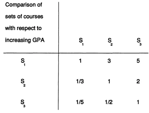
It is helpful to frame the comparison question so that the answer is a whole number. In the example, if the student started out comparing S3 to S^, they would just reverse them to obtain the value of 5 and then determined the required 1/5. To continue with the example, the student makes all pairwise comparisons and arrives at the following judgemental matrix. Comparison of sets of courses with respect to increasing GPA s 1 S2 S3 S 1 1 3 5 S 2 1/3 1 2

s

Figure 2.2.3 GPA Judgmental Matrix

The AHP determines the priorities of each alternative, that is, the importance or weight to be given each

the advanced mathematical theory of eigenvalues and

eigenvectors. The decision maker need not delve into the topic here except to note that the AHP interprets the eigenvector associated with the largest eigenvalue as the priorities that indicate the importance of each alternative in accomplishing the objective. For a matrix with n rows and columns, the student can approximate the required priority eigenvector as follows. For each row i of the matrix, take the product of the ratios in that row and denote it by IIi( Calculate the corresponding geometric mean Pi7 where Pi = Hi. Let P = ]TiPi. The student

normalizes the Pi by forming Pi = Pi/P. Each p± is the ith priority or weight given to the ith alternative. The

calculations for the GPA judgement matrix are shown in figure 2.2.4.

The AHP interprets this information as indicating that the set of courses Si will contribute the most to

increasing the GPA, followed by S2, and finally S3. Based on the magnitudes of the Pi, the senior should feel

comfortable in chosing Si, select S2 with caution, and should not select S3.

Making the problem a bit more interesting, the student still must select one of the three sets of courses, but the student is concerned with more than just GPA. Now the

GPA _s. s 2 s 3 n p = p.-FJ/P

S 1 3 5 15 2.466 0.65

S 1/3 1 2 0.667 0.874 0.23

S 1/5 1/2 1 0.1 0.464 0.12

P = 3.804

The priorities for the courses are then

P. s , 0.65 s 2 0.23 s 3 0.12

Figure 2.2.4 Computed GPA Judgement Matrix

But, in selecting a set of courses, there are general

criteria that need to be considered. The criteria deal with how the various sets of courses contribute to GPA

improvement, advancing the student in the major career field, and giving the student a broader educational background. This new problem can be pictured in the

Level 1: Focus (goal)

Level 2: Criteria

Level 3: Alternatives

Improve GPA Advance career Broaden education Excellent education

Figure 2.2.5 GPA Three Level Hierarchy

Unlike the previous two level hierarchy example, here the student first needs to determine how important each criterion is in achieving the objective of an excellent education. The student can do this by constructing a

judgment matrix as before and comparing the criteria

pairwise by asking the question: Of the two criteria, which is considered more important in contributing to the focus and how much more important is it? Using the pairwise comparison scale, the student determined the judgment

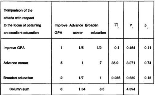
Comparison of the criteria with respect to the focus of obtaining an excellent education

Improve Advance Broaden GPA career education

TT f P Pi Improve GPA 1 1/5 1/2 0.1 0.464 0.11 Advance career 5 1 7 35.0 3.271 0.74 Broaden education 2 1/7 1 0.286 0.659 0.15 Column sum 8 1.34 8.5 4.394

Figure 2.2.6 Three Level Computed Pj_

From the p^ column, the student can see that the

advance career criterion has a much higher priority (0.74) than the other two. Each of the other criteria is about the same in their importance to the objective. The student next has to carry out the analysis of the third hierarchy, that is, determine the importance of the sets of courses to each criterion. For example, for the criterion improve GPA, the student needs to ask the question: Of the two sets of

courses being compared, which is considered more important in improving GPA and how much more important is it? The

student asked similar questions for the other two criteria and arrive at three judgment matrices/ as given below.

GPA s_{1 S 2 S 3} TT _{P , P,} S₁ 1 3 5 15 2.466 0.65 S 2 1/3 1 2 0.667 0.874 023 S 3 1/5 1/2 1 0.464 0.464 0.12 3.804 Advance career s_{1 S 2 S 3} n P 1 P. S 1 1/2 8 4 1.587 0.36 S 2 2 1 9 18 2.621 0.59 S₃ 1/8 1/9 1 0.0139 0.240 0.05 4.448 Broaden education S , S 2 S » n P, P. s , 1 6 1/5 1.2 1.063 0.27 S 2 1/6 1 1/3 0.0556 0.382 0.10 s₃ 5 3 1 15 2.466 0.63 3.911 Figure 2.2.7 Three Level Judgment Matrices

From the GPA judgment matrix the student can see that the set of courses S1 with Pi = 0.65 contributes the most to achieving the GPA criterion and S3 (p3 = 0.12) the least; from the advance career matrix, S2 (P2 = 0.59)

contributing the most to that criterion and S3 (p3 = 0.05) the least; and from the broaden education matrix, the

student has S3 (p3 = 0.63) being the set of courses that would contribute the most to broadening their education and s2 (P2 = 0*10) the least.

Based on the above analysis/ it appears as if a good job was done in forming the three alternative sets of courses; one is better for each criterion. But their contributions to achieving the other criteria are rather varied and in some cases quite weak. The student is still not in a position to pick a set of courses because the influence of the criteria must still be factored in. Based on the earlier level two analysis, the criteria are not equal in terms of the goal of achieving an excellent

education. The student then determines weights of 0.11 to improve GPA, 0.74 to advance career, and 0.15 to broaden education. These weights are used to modify the

corresponding level three weights for each of the courses. The student first organizes the results obtained so far in figure 2.2.8.

To obtain the composite hierarchical priority for an Si, the student must multiply each of its level 3

priorities by the corresponding level 2 priority and sum the products. For Si

px = (0.11) (0.65) + (0.74) (0.36) + (0.15) (0.27) = 0.38 and for S2 and S3 respectively,

p3 = (0.10) (0.12) + (0.74) (0.05) + (0.15) (0.63) = 0.14

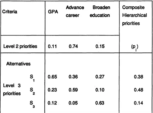
Criteria GPA Advance

career Broaden education Composite Hierarchical priorities Level 2 priorities 0.11 0.74 0.15 _(P.) 1 Alternatives S 1 Level 3 s priorities 2 0.65 0.36 0.27 0.38 0.23 0.59 0.10 0.48 S 3 0.12 0.05 0.63 0.14

Figure 2.2.8 Three Level Composite Priorities

The theory of the AHP is that these final composite weights capture the senior's explicit and implicit knowledge about each set of courses in terms of their satisfaction of the individual criteria and of the senior's feelings as to the importance of the criteria in achieving the ultimate goal of obtaining an excellent education. For the student's decision problem of selecting the set of courses for achieving the best education, the composite indicates

that the set of courses S2 would be the best choice (p2 =0.48), with set Sx (px = 0.38) the next best. The set S3, although being best in terms of broadening education, does little to improve total education (p3 = 0.14)

Z^2L

ABE Scale

The ability of the scale 1-9 to express feelings as to the intensity of a pairwise comparison is based on

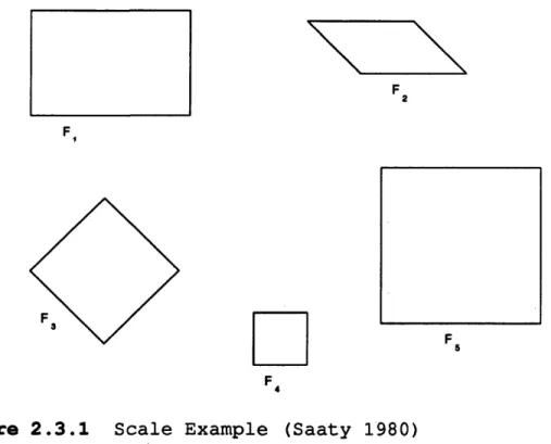
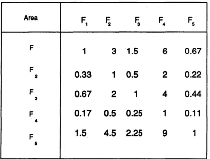
psychological measurement studies (Saaty, 1982) In turn, the validity of the total AHP process has its roots in the quantification of physical attributes using human sensory perceptions. To demonstrate how the AHP can be used to estimate a physical attribute, consider the following geometrical problem illustrated by the figures Fr, F2, F3, F4, and F5 in figure 2.3.1.

Let the unknown area of figure be denoted by and the total area covered by all five figures be T = A x + A2 + A3 + A 4 + A 5. Estimate how much of the total area is

contained in each figure, that is, determine the

proportions Aj/T. The only measurement tool that is allowed to be used is visual perception. To use the AHP, visually compare each figure pairwise with the others by asking the question: Of the two figures being compared, which one has

the larger area and how much larger is it? For example, it is clear that F1 is larger than F4, but is the ratio 2 to 1, 3 to 1, 4 to 1, or what? The answer should be entered in the comparison matrix for Fx against F4, and the

reciprocal for F4 against F ^ Develop the comparison matrix

F 2 F_i

Figure 2.3.1 Scale Example (Saaty 1980)

for the figures using the intensity numbers 1 to 9 and their reciprocals, and calculate the associated priorities. Fractional priority values should, hopefully, come close to the actual ratios of A^/T. The following figure could be

the comparison matrix for the problem with a person using their visual perception.

Area F1 F2 FS F 4 Fs F 1 3 1.5 6 0.67 F 2 0.33 1 0.5 2 0 .2 2 F 3 0.67 2 1 4 0.44 F 0.17 0.5 0.25 1 0.11 4 F 1.5 4.5 2.25 9 1 5

Figure 2.3.2 Actual Scale Comparison

Here the element in the ith row and jth column a^j = Ai/Aj, where the and Aj values are the correct area

values. Using the above matrix to determine more accurate values results in px = 0.27, p2 = 0.09, p3 = 0.18, p4 = 0.05, and p5 = 0.41,

2.4 Consistency

For the AHP, Saaty proposes the calculation of

consistency index that measures how consistent the decision maker is in comparing the elements in a judgement matrix

(Saaty 1980) When the decision maker has many factors to compare, it is difficult to maintain such consistency, and, based on intuitive and other factors, the decision maker might want to deviate from true consistency. As Saaty

notes, people may not be perfectly consistent, but that is the way people tend to work (Saaty 1982) Certainly gross inconsistency would lead to invalid results. Based on certain mathematical relationships, there is a simple way to measure consistency of AHP judgement matrix. It is derived from the properties of judgment matrices and the theory of eigenvalues and eigenvectors. A consistency

measure is determined in the following manner. Consider an AHP judgment matrix with n rows and columns, that is,

a ll . a ln

a nl a nn

corresponding p.^, Sum the n products and denote the results by zmax. The formula is

n n n

zmax = Pi* H ail + P2*

Y

Y

i=l i=i i=l

This is an approximate way of calculating the maximum eigenvalue of the matrix. If the matrix is consistent, then

zmax = n « Thus, a suggested consistency index (Cl) is

CI = (zmax “ n)/(n - 1)

The CI is compared to the corresponding random consistency index (RI) from figure 2.4.1,

It is suggested that if the consistency ratio CR = CI/RI is less than or equal to 0.10, then the results be accepted. Otherwise, the problem should be studied again and the judgment matrix revised. The judgment matrix should have zmax => n. Also, matrices of orders 1 and 2 are

necessarily consistent and the CI and CR formulas are not applicable.

The decision maker can illustrate the CI and CR calculation for the level 2 judgment matrix used in deciding which set of courses to take. From figure 2.2.6

Size of

matrix (n) 1 2 3 4 5 6 7 8 9 1 0

Rl 0.00 0.00 0.58 0.90 1.12 1.24 1.32 1.41 1.45 1.49

From Thomas L. Saaty, The Analytic Hierarchy Process,

Based on study from Oak Ridge National Laboratory

Figure 2.4.1 Random Consistency Index

zmax “ (0.11) (8) + (0.74) (1.34) + (0.15) (8.5) = 3.15

CI = (3.15 - 3)/ (3-1) = 0.075

CR = CI/RI = 0.075/0.58 = 0.129

As the CR is close to 10%, the priorities are acceptable. The total CI of a hierarchy is obtained by weighting each CI by the priority of the element with respect to which the comparison is being made and then adding all the results.

Thus, if a CI is high it might not have much influence due to its multiplier. This, for example, would be the case in the education problem if the GPA matrix had a high CI. The hierarchy CR is obtained by comparing the hierarchy CI to the hierarchy RI, which is found by summing similarly weighted RI's, where each RI corresponds to the dimension of the related individual CI. The hierarchy CR should be about 0.10.

When applying the AHP to decision problems that involve people judging qualitative factors, the decision maker should not expect to obtain a consistent judgment matrix. In fact, for such problems, strict consistency implies a rigidity in the decision maker's estimate that would not allow them to factor in new information.

Certainly, gross inconsistency needs to be avoided, but do not be afraid to let judgment rule the comparisons.

If a judgment matrix has a CR greater than 0.10, there is a way to find out which comparison seems to be the ones causing the trouble. Denote the numbers in the original nth order comparison matrix by a ^ (the element in the ith row and jth column) and the associated priorities by Form a new matrix in which element (i, j) is given by Pj_/Pj. This resultant matrix will be consistent and produce the

original pi( Take the ratio of each a ^ to its

the value of 1.0 probably have a±j values that need

adjusted. As the decision maker is not looking for complete consistency, Saaty suggests only adjusting the a^j that corresponds to the ratio with the largest absolute

deviation from 1.0 (Saaty 1980) If the ratio is greater than 1.0, adjust a^j down by one unit; if the ratio is smaller than 1.0, adjust the aij up by one unit.

2,.,5 Group Interaction

The AHP can be used successfully within a group. Brainstorming and sharing of knowledge can lead to better representation and solution to the problem than a single person might. In group participation the members structure the problem, provide the judgments, debate the judgments, and make a case for their values. In the best situation the group is small and all members of the group are well

informed, motivated, and want to solve the problem. The group members must also be willing to participate in a structured process whose outcome could effect them in future activities.

The process cannot be set in a list of rules. The process must remain flexible to stimulate the participates thought process to provide input to the process. The group

must be familiar with how AHP works and how their input can assist in solving the problem. A good way to begin the

session is by brainstorming to come up with the main focus of the problem. Once the problem has been identified and agreed upon the hierarchy for the problem can be

established. Breaking down a complex issue into different levels is useful for a group with widely varying

perspectives. Each member can present their own opinions for the hierarchy, no matter what the level may be. Then the group assist in identifying the overall structure of the issue. The group then agrees on how it will proceed to make decision. The whole group may participate at each level or they may be delegated to subgroups the

responsibility of considering or setting priorities for different levels.

The process of setting the priorities among the criteria in a group can sometimes involve interaction, bargaining and persuasion. In a large group the process of setting priorities may be easier to handle by dividing the group into smaller elements that specialize in a particular subject. When the subgroups rejoin then the values in each matrix can be analyzed and revised if needed. If the values are different they can be combined into one solution by forming the geometric mean of the values. The values are multiplied and a root equal to the number of individuals

who provide the values is taken. For example, the geometric mean of 2, 3, and 7 is -^2*3*7, which is 3.48 (rounded to 3 on the pairwise comparison scale) Taking the geometric mean of individual judgments is one way to resolve a lack of consensus on values if a compromise cannot be reached.

Some groups may be composed of people with different experience, values, and status in the organization. A superior in the organization may be unwilling to

participate in the process if their input is rated equally with the subordinates. This can be overcome by

establishing a hierarchy to weight the votes of each individual. Votes may not have to be weighted if the interaction process allows individuals to exercise their influence through debate even when the votes are equally weighted.

As the process continues people may change their judgments as a result of gathering more information or by reevaluating their opinions. AHP can be useful if the

priorities and the outcomes of decisions change even within a short time. It can also provide an opportunity to

identify variables subject to change and attain certain priorities to those changes. An example and discussion of the AHP sensitivity is given in chapter three. AHP should be looked at as a continuing document that is never

finished. It is not applied just one time, but continues to grow and change with the problem.

Sometimes people are not willing to reveal their true preferences and may have a hidden agenda item. If people do not to state their opinions, the problem will be incomplete and the analysis and priority setting will be inadequate. To try and overcome this shortcoming include enough members in the group to produce a broad range of ideas.

As a group becomes more experienced in using the AHP, consistency and speed should improve. The stake of members is another important factor. If the group members have a genuine interest and have some risk in the outcome of the process, they should be more willing to see the process succeed in making a correct decision. Most of the problems in applying AHP in a group setting is with the pairwise comparison of the criteria. The process should be used on smaller, better defined problems when used for the first time. Applying the group session in the military problem will be discussed in chapter four as an area for further

study.

2.6 Justification The Method

Assume that n activities are being considered by a group of interested people. Assume that the group's goals

are:

(1) to provide judgments on the relative importance of these activities;

(2) to insure that the judgments are quantified to an extent which also permits quantitative

interpretations of the judgments among all activities.

The decision maker's goal is to describe a method of

deriving, from the group's quantified judgments, a set of weights to be associated with individual activities. These weights should reflect the group's quantified judgments. What AHP achieves is to put the information resulting from

(1) and (2) into a usable form without deleting information residing in the qualitative judgments.

Let Ci, C2/ . ,Cn be the set of activities. The quantified judgments on pairs of activities C^, Cj are represented by an n-by-n matrix

A — , (i/j = 1/2, , ., n)

The entries a ^ are defined by the following entry rules. Rule 1 If aij = h, then aj^ = 1/h, h = 0.

Rule 2. If Ci is judged to be of equal relative importance as Cj, then a ^ = 1, a ^ =1; in particular, a ^ = 1 for all i , Thus the matrix A has the form

A = 1 1/ a12 a 12 1 lz n a 2 n l / a ln ^-/a 2n ' 1

Having recorded the quantified judgments on pairs (Ci,Cj) as numerical entries a ^ in the matrix A, the problem now is to assign to the n contingencies

ClfC2, ■» ► /Cn a set of numerical weights w1# w2, ./Wn that would reflect the recorded judgments.

In order to do so, the vaguely formulated problem must first be transformed into a precise mathematical one. This essential step is the most crucial one in any problem that requires the representation of a real life situation in terms of an abstract mathematical structure. It is crucial in the present problem where the representation involves a number of transitions that are not immediately apparent, The major question is the one concerned with the meaning of the vaguely formulated condition in the statement of the goal: "these weights should reflect the group's quantified judgments." This presents the need to describe in precise, arithmetic terms, how the weights Wi should relate to the judgments a^; or the problem of specifying the conditions wish to impose on the weights the decision maker seeks in relation to the judgments obtained. The desired

description is developed in three steps, proceeding from the simplest special case to the general one.

Step 1 Assume first that the judgments are merely the results of precise physical measurements. Say the judges are given a set of pebbles, Clf C2r .... t Cn and a precision scale. To compare Cx with C2, they put Cx on a scale and read off its weight say, ^ = 305 grams. They weigh C2 and find w2 = 244 grams. They divide Wi by w2 and set 1.25.

They pronounce their judgment, C1 is 1.25 times as heavy as C2 and record it as a12 = 1.25. Thus, in this ideal case of exact measurement. The relationships between the weights wA and the judgments a±j are simply given by

w±/wj = a±j (for i, j = 1,2, .,n) (1-1) and A = Wi/w-l w2/wi wi/w2 w2/w2 W n / W i w n / w ; Wi/Wn w2/wn wn/wn

relationships to hold in the general case. Imposing these stringent requirements would make the problem of finding the unsolvable. First, even physical measurements are never exact in a mathematical sense; second, allowance must be made for deviations; and finally because in human

judgments, these deviations are considerably larger.

Step Z in order to see how to make allowance for

deviations, consider the ith row in the matrix A. The entries in that row are

a il' a i2' a ij' •' a in

In the exact case these values are the same as the ratios

W i / W i , W i / w 2 , . o •, w ± /wj, , , w ± / w n

Hence, in the ideal case, multiply the first entry in that row by w1# the second entry by w2, and so on, the group would obtain

(Wi/Wi) * W X = W ± , (W± / W 2 ) * W 2 = W ± , (W± /Wj) *W j = w ± , ,, (wi / w n ) * w n = W i

The result is a row of identical entries w±, w±, w±

In the general case, the group would obtain a row of entries that represent a statistical scattering of the values around Wi« It appears, therefore, reasonable to require that wi should equal the average of these values.

Instead of the ideal case (1-1)

w± = a±jW±j (i, j = 1,2, . ,n)

the more realistic relations for the general case take the form

Wi = the average of (ajjWi, ai2w2, . ., ainwn^ (1”2) While the relations in (1-2) represent a substantial relaxation of the more stringent relations (1-1), there still remains the question: is the relaxation sufficient to insure the existence of solutions; that is, to insure that the problem of finding unique weights wA when the aij are given is a solvable one?

Step 2. To find the answer to the above mathematical

questions, it is necessary to express the relations in (1- 2) in still another, more familiar form. In seeking a set of conditions to describe how the weight vector w should relate to the quantified judgments, first consider the ideal exact case in Step 1, which suggested the relation

(1-1) Next, realizing that the real case will require allowances for deviations, provided for such allowances in Step 2, leading to the formulation (1-2) Now, this is

still not realistic enough; that is, that (1-2) which works for the ideal case is still to stringent to secure the

existence of a weight vector w that should satisfy (1-2) Note that for good estimates a^j tends to be close to Wj/Wj

and hence is a small perturbation of this ratio. Now as a ^ changes it turns out that there would be a corresponding solution of (1-2), if n are also to change. Denote this value of n by zmax. Thus the problem

n

wi = i/Zmax* Z <aijwij> i = 1/ ./n j=l

has a solution that also turns out to be unique. This is an eigenvalue problem with which the problem will be dealing with.

In general, deviations in the a±j can lead to large deviations both in zmax and in wifi = 1, .., n. This is not the case for a reciprocal matrix which satisfies rules 1 and 2, In this case the group has a stable solution.

Briefly stated in matrix notation, start with what is call the paradigm case Aw = nw, where A is a consistent matrix and consider a reciprocal matrix A' which is a perturbation of A, extracted from pairwise comparison judgments, and solve the problem A'w' = zmaxw' where zmax is the largest eigenvalue of A'

The analytic hierarchy process reflects the way people naturally think and addresses complex problems on their own terms of interaction. Through a mathematical sequence it synthesizes their judgements into an overall estimate of the relative priorities of alternative courses of action.

It also tracks inconsistencies in the judgements, enabling leaders to assess the quality of the stability of the

solution. The best aspect of the AHP is the fact that it allows decision makers the opportunity to incorporate intangible factors into the process. This unique feature will enable the military commander to compute combat power, that in the past has been difficult to grasp because of the intangible factors involved in its computation. In the next chapter of this thesis the AHP will be applied to the

Chapter 3

Military Application

As defined in chapter one, combat power is a complex combination of tangible and intangible factors of the battlefield. CGSC ST 100-9, The Command Estimate.

explains how a simple comparison of the number of units would be inappropriate since the capabilities of units vary. Therefore, at each level, the planner must determine the overall combat power of the type units being compared. To accomplish this, a base unit must first be selected. A subjective evaluation must then be made of all other types of units relative to the base unit using the tangible and intangible factors of combat power. The Analytical

Hierarchy Process (AHP) is perfectly suited for dealing with combat power since the method also deals with both tangible and intangible factors, effectively arriving at a decision.

One major problem, which has been unsolved until recently, is how to deal with the intangible factors that arise in computing combat power, In the past, people have talked around intangibles and have concluded that dealing with them is highly subjective. Intangibles can be compared according to preference priority and can be made part of a large framework that incorporates both the tangible and

concrete and the intangible and abstract factors that bear on the problem (Saaty 1989) The Analytic Hierarchy

Process, developed by Saaty in the 1970s provides such a framework. AHP has been used to analyze complex conflicts, such as the Falkland Island crisis and the Iran hostage rescue operation, but here the complexity of the conflict will be reduced to the company level, It should be noted that AHP is a simple process that can work not only with small problems, but can also grow with the problem as the complexity of it is increased. The military problem

presented here revolves around a tank company commander deciding which platoon in the company has the most combat power and how it will be assigned against enemy Avenues of Approach. The first step is to assess the company's

platoons against each other to calculate the combat power of each. This will be done using AHP to rank the priority of each platoon against a set of criteria. After this has been done a quick and dirty method, based on Saaty's

pairwise comparison table, will be introduced to assist the commander in speeding up the process of computing combat power. The next step will be to assign the company's platoon against enemy avenues of approach. The criterion

comparison of the first AHP problem will be used to rank the platoon and avenue of approach alternatives in this

step. Last the ranking of the alternatives from above will be used to assign the platoons to enemy avenues of

approach. In this chapter these three ideas, AHP, quick and dirty, and platoon assignment, will be used to solve the problem of what combat power really is.

To use AHP in making a decision the user does not necessarily need to understand why AHP works but should be knowledgeable of the subject matter being used with AHP. Otherwise, the results may not yield the correct decision, therefore, it is important to understand the doctrine and responsibilities with which a company commander must deal with.

3.1 Command

The commander's estimate of the situation is an

integral part of planning process for conducting military operations. It is used by the commander to collect and analyze relevant information for developing the most

effective solution to a tactical problem within the limits of time and available information. At company level the commander's estimate of the situation is a mental process which provides a format for the logical analysis of all relevant factors (FM 71-1 1987) An integral part of the commander's estimate is the calculation of combat power and

assignment of that combat power against enemy avenues of approach. Mentally calculating these can often lead to a wrong analysis of situation. It is here that AHP can reduce the work load of the commander and help them produce a

decision that the commanders can assure themselves is the best possible. If time is available a detailed calculation should be performed to ensure the best possible analysis of the situation.

It is essential at company level that the commander understands the concept of combat power. As stated before, power is composed of both tangible and intangible factors and if one of the factors is not considered in the analysis the conclusion maybe incomplete. The AHP method of

computing and assigning combat power presented here could easily be integrated into the company commander's planning process. This would change the analysis from a mental process without any guidance, to a mathematical process that will insure a detailed analysis of the situation.

3.2 combat Rower

Because company commanders are at the lowest level of command, they can accurately calculate combat power with more detail than higher level commanders. The commander

is very familiar with the capabilities, both tangible and intangible, of each individual, crew, and tank under their command. As a result they are able to use some of the human dimensions that higher commanders cannot.

Basically combat power is merely a numeric value that a commander assigns to the unit to evaluate it against enemy forces. There are many factors, called combat

multipliers, that go into computing combat power many of which are intangible and difficult to define. Without all these factors comparing platoons would be inappropriate since the equipment and capabilities are different in each. The combat criteria that are used in AHP should be

carefully selected by the company commander in order that they can evaluate the unit in an accurate manner. There are numerous combat criteria that can be used, but it is up to the commander to select those that are essential to the unit's mission.

3.3 Combat Criteria

Although the combat criteria can change from situation to situation the commander will select the criteria that are seen as essential to the completion of the mission.

The following combat criteria will be used to evaluate the units combat power in this example:

* Equipment * Tank Gunnery * Engineer Support * Offense/Defense * Firing Modes * Crew Strength

3 .4 Analytic Hierarchy Process

Chapter two explains the analytic hierarchy process which begins by laying out the elements of the problem as a hierarchy. Next, a paired comparison among the elements of a level is required based on the criteria of the next

higher level, These comparisons gave rise to priorities and finally to overall priorities. Consistency is also

measured. These basic steps of the process will now be implement for the military problem and how it relates to combat power.

The commander must decide which of the platoons has the highest combat power based on the criteria already presented. Some of the platoons performed well at tank gunnery while others did not. Also the operational modes of

the firing computers and the crew strength are different among the platoons. The commander does have some

flexibility in assigning all or part of the combat

engineers to one or all of the platoons. The relationship between goal of combat power, criteria, and the three

platoons can be pictured in a three level hierarchy diagram as in figure 3.4.1, Firing mode 3rd platoon 2nd platoon 1st platoon Engineer support Crew strength Tank gunnery Equipment

Selecting Combat Power

Figure 3.4.1 Combat Power Hierarchy

First determine how important each criterion is in achieving the objective of rating the combat power of the

platoons. Do this by constructing a judgment matrix as in chapter two and comparing the criteria pairwise by asking the question: Of the two criteria, which should be

considered more important in contributing to the focus and how much more important is it? Using the pairwise

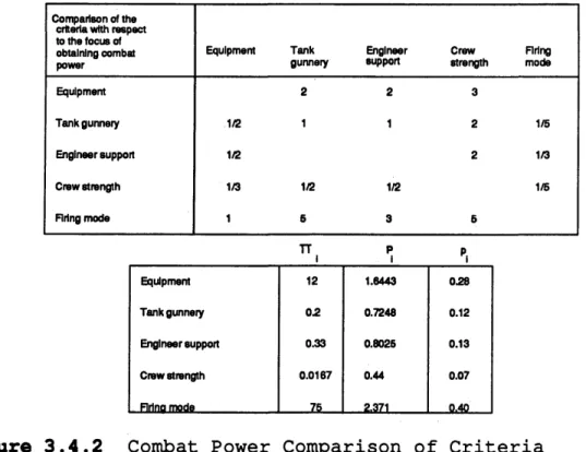
comparison scale the commander determines the judgment matrix and calculated pA as shown in figure 3.4.2.

Comparison of the criteria with respect to the focus of obtaining combat power Equipment Tank gunnery Engineer support Crew strength Firing mode Equipment 2 2 3 Tank gunnery 1/2 1 1 2 1/5 Engineer support 1/2 2 1/3 Crew strength 1/3 1/2 1/2 1/5 Firing mode 1 5 3 5 TT l PI P. Equipment 12 1.6443 0.28 Tank gunnery 02 0.7248 0.12 Engineer support 0.33 0.8025 0.13 Crew strength 0.0167 0.44 0.07 Flrlnci mode 75 2.371

Figure 3.4.2 Combat Power Comparison of Criteria

From the p^ column, the firing mode criterion has a much higher priority (0.40) than the other four, Equipment

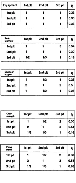
is slightly higher and the other three are about the same. Next the commander needs to carry out the third level of the hierarchy, that is , determine the importance of the three platoons to each criterion. This is done by

constructing five judgment matrices, one for each

criterion. For example, for the criterion tank gunnery, the commander ask the question: Of the two platoons being compared, which is considered more important in computing combat power and how much more important is it? The

commander must then ask a similar question for the other five criteria to arrive at the five matrices given in figure 3.4.3.

From the equipment judgment matrix the platoons all have a pi = 0.33 contributing the same to achieving the equipment criterion and from the tank gunnery matrix, 1st platoon (p2 = 0.54) contributing the most to that criterion and 3rd platoon (p3 = 0.16) the least. From the engineer support matrix, 1st and 3rd platoon both (Pi,2 = 0.25) being the platoons that contribute the least to engineer support and 2nd platoon (p2 = 0.50) the most. From the crew strength matrix 2nd platoon (p2 = 0.54) contributing the most to the criterion and 3rd platoon (p3 = 0.16) the

least. From the last criterion matrix, firing mode, 2nd platoon (p2 = 0.54) being the platoon that would contribute

Equipment 1st pit 2nd pit 3rd pit _R 1st pit 2nd pit 3rd pit 1 1 1 1 1 1 1 1 1 0.33 0.33 0.33 Tank

Qunnary 1st pit 2nd pit 3rd pit R 1st pit 1 2 3 0.54 2nd pit 1 1 1 0.30 3rd pit 1/2 1/3 1 0.16

Enginaar

aupport 1st pit 2nd pit 3rd pit R 1st pit 1 1/2 1 0.25

2nd pit 2 1 2 0.5

3rd pit 1 1/2 1 0.25

Crew

strength 1st pit 2nd pit 3rd pit R 1st pit 1 1/2 2 0.30 2nd pit 2 1 3 0.54 3rd pit 1/2 1/3 1 0.16

Firing

mode 1st pit 2nd pit 3rd pit R 1st pit 1 1/2 2 0.30 2nd pit 2 1 3 0.54 3rd pit 1/2 1/3 1 0.16

the most to the firing mode criterion and 3rd platoon (p3 = 0.16) the least,

Based on the above analysis, it appears that a good job was done in forming the three alternative platoons; one is better in each criterion except for the equipment

criterion. This is due to the fact that all three platoons have exactly the same type of equipment; however, once the enemy force's equipment is introduced to the problem this criterion will have more of an impact. The influence of the criteria must be factored in before the platoons can be rated for their combat power. Based on the earlier level 2 analysis, the criteria are not equal in terms of the goal of rating the platoons combat power. The weights of 0.28 for equipment, 0.12 for tank gunnery skills, 0.13 for support from the engineers, 0.07 for the strength of the crew, and 0.40 for the tanks firing mode are determined by the level 2 analysis. These weights are used to modify the level 3 weights for each platoon. The results are organized in figure 3.4.4.

To obtain the composite hierarchical priority for the platoons, multiply each of its level 3 priorities by the corresponding level 2 priority and sum the products. For 1st platoon