2011:09 Is Copper Immune to Corrosion When in Contact With Water and Aqueous Solutions?

(1)

Report number: 2011:09 ISSN: 2000-0456 Available at www.stralsakerhetsmyndigheten.se

Is Copper Immune to Corrosion

When in Contact With Water

and Aqueous Solutions?

2011:09

Authors: Digby D. Macdonald

Samin Sharifi -Asl

(2)

(3)

SSM perspective Background

The KBS-3concept implies that spent nuclear fuel is placed in copper canisters surrounded by clay and finally placed approximately 500 m down from surface into granitic bedrock, in order to isolate the spent nuclear fuel from humans and environment for very long time scales (i.e. millions of years). The concept is based on the multi-barrier principle, in this respect the barriers are the copper canister, clay material and finally the granitic bedrock. All barriers will work alone and together in order to retard the spent nuclear fuel to enter into the biosphere. In this report it is only degra-dation of the first barrier, the copper canister that is considered.

The mechanisms of copper corrosion in the planned repository for spent nuclear fuel according to the KBS-3 concept need to be fully understood in order to review the license application in an authoritative way. Copper as a canister material was chosen by SKB already 1978 in the KBS-2 report. The main reasons for selecting copper were 1) copper is thermodynamically immune in the presence of pure anoxic water, and 2) copper has sufficient mechanical strength to resist all plausible mechanical loads present in the repository. Thermodynamically, immunity of copper in pure anoxic water implies that copper will not corrode in the presence of pure anoxic water. The reason for why copper cannot corrode in the immune state is that this will cause a positive change in the Gibbs Energy. This contradicts the se-cond law of thermodynamics, which states that for a spontaneous reaction to occur the change in Gibbs Energy has to be negative.

The water present at the repository depth in the proposed site at Forsmark is of course not pure water. At repository depth different dissolved species like sulphide in the water will cause corrosion of copper. It is a fact that the reaction between copper and sulphide occurs under a negative change in Gibbs Energy, this was also recognized by SKB in the KBS-2 report. The rate of copper corrosion at repository depth will hence be controlled by either the rate of transport of corroding species to the canister or the rate of trans-port of corrosion products from the copper surface, or both.

Objectives

The aim of this project has been to increase knowledge and to contribute to the research community in the area of copper corrosion in a repository en-vironment. For SSM, the most important subject is to provide better condi-tions for a science based evaluation of a repository for spent nuclear fuel. In this respect, this project aimed at conducting a comprehensive theoretical study on corrosion of copper in repository environment based on an expec-ted composition of dissolved species in the groundwater in the Forsmark area. In addition the thermodynamic immunity of copper in pure anoxic water has been especially addressed as this was one of the initial conditions made by SKB for selecting copper as canister material.

(4)

Results

The authors have shown, in so-called corrosion Domain Diagrams, that copper in a thermodynamic sense can be considered as immune in pure anoxic water (without dissolved oxygen) only under certain conditions. It is shown that copper will corrode in pure anoxic water with very low concentrations of [Cu+_{] and very low partial pressures of hydrogen gas.}

At higher concentrations of [Cu+_{] and partial pressures of hydrogen,}

copper is found to be thermodynamically immune and will not corrode. The rate of copper corrosion in the repository water environment will thus depend on the transport of corrosion products away from the cop-per surface or the transport of corroding species to the copcop-per surface. The degree to which this affects the corrosion of copper canisters in the repository environment has not been further studied. Still, the result shows that copper cannot be considered as thermodynamically immune in the presence of pure anoxic water, this implicate that one of SKB:s initial conditions for selecting copper as a canister material can be questioned. To what degree this may influence the corrosion of copper canisters in the repository environment still needs to be investigated. Of other species present in the water at repository depth in Forsmark, different sulphur species was found to be most deleterious causing cop-per to corrode in an anoxic environment under hydrogen gas evolution. In order to find out what species that can be present in a repository environment a Gibbs Energy Minimisation algorithm was employed. By this method it was concluded that (S2_{-, HS- and H}

2S) are predicted to be

present in the entire anoxic period at sufficient concentrations to cause corrosion of copper. It is finally concluded that the corrosion rate of copper canisters will be determined by the very complex interaction bet-ween copper, buffer material and bedrock in order to reduce corrosion of copper to an acceptable level.

Need for further research

In order to provide a better understanding of copper corrosion pro-cesses more work is needed to understand the system that forms com-plexes with copper in an expanded concentration interval of species in groundwater. The evolution of corrosion damage during the lifetime of the repository need to be understood more in detail before a realistic as-sessment of copper corrosion in repository environment can be made. Project information

Contact person SSM: Jan Linder Reference: SSM 2010/531

(5)

2011:09

Authors: Digby D. Macdonald and Samin Sharifi-Asl

Center for Electrochemical Science and Technology Department of Materials Science and Engineering Pennsylvania State University, USA

Date: March 2011

Report number: 2011:09 ISSN: 2000-0456 Available at www.stralsakerhetsmyndigheten.se

Is Copper Immune to Corrosion

When in Contact With Water

and Aqueous Solutions?

(6)

This report concerns a study which has been conducted for the Swedish Radiation Safety Authority, SSM. The conclusions and view-points presented in the report are those of the author/authors and do not necessarily coincide with those of the SSM.

(7)

List of Figures

Figure 1: Corrosion domain diagram for copper in water as a function of temperature………16 Figure 2: Corrosion domain diagram for copper in water + HS- as a function of temperature…………..18 Figure 3: Corrosion Domain Diagram for copper in the presence of the polysulfide, S3

2-_……….20

Figure 4: Structure of the trithiosulfate anion……….…20 Figure 5: Corrosion Domain Diagram for copper in the presence of HS3O3

-. Note that this species is a powerful activator of copper………22 Figure 6: Corrosion Domain Diagram for copper in the presence of S4O3

2-. Note that this species is predicted not to activate copper………...23 Figure 7: Volt-Equivalent Diagram for sulfur in Forsmark ground water, pH = 7, [S] = 10 ppm, 25°C. The red point represents elemental sulfur………....32 Figure 8: VED for the sulfur-water system at 125oC, pH = 9, [S] = 0.001 ppm………34

Figure 9: Calculated hydrogen pressure from the reaction,

3Fe2SiO4(F)+2H2O(l)=2Fe3O4+3SiO2+2H2(g)……….……….……37 Figure 10: Calculated hydrogen pressure from the reaction, 3Fe(OH)2=Fe3O4+2H2O(l)+H2(g)……..…38 Figure 11: Calculated hydrogen pressure from the reaction, Cu + H(+) = Cu(+) + 0.5H2(g),

m(Cl-)=0.169………..……….43

Figure 12: Calculated hydrogen pressure from the reaction, Cu + H(+) = Cu(+) + 0.5H2(g),

m(Cl-)=0.338………..43

Figure 13: Calculated hydrogen pressure from the reaction, Cu+H(+a)+Cl(-a) = CuCl(s) + 0.5H2(g),

m(Cl-)=0.169……….………...44

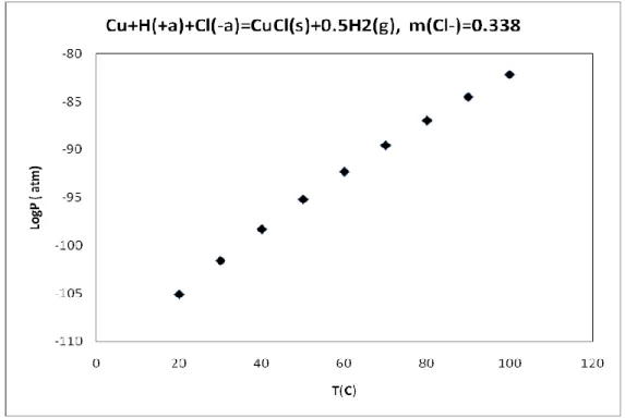
Figure 14: Calculated hydrogen pressure from the reaction, Cu + H(+a)+Cl(-a) = CuCl(s) + 0.5H2(g),

m(Cl-)=0.338………44

Figure 15: Calculated hydrogen pressure from the reaction, Cu + H(+a)+Cl(-a) = CuCl(a) + 0.5H2(g),

m(Cl-)=0.169………....45

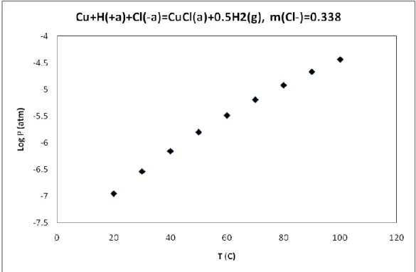
Figure 16: Calculated hydrogen pressure from the reaction, Cu + H(+a)+Cl(-a) = CuCl(a) + 0.5H2(g),

m(Cl-)=0.338………..………45

Figure 17: Calculated hydrogen pressure from the reaction, Cu + H(+a)+2Cl(-a) = CuCl2(-a) + 0.5H2(g),m(Cl

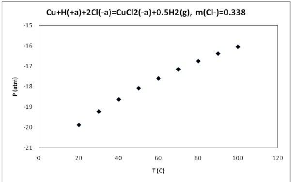
-)=0.169………46 Figure 18: Calculated hydrogen pressure from the reaction, Cu + H(+a)+2Cl(-a) = CuCl2(-a) +

0.5H2(g), m(Cl-)=0.338………46

(9)

3

Figure 19: Calculated hydrogen pressure from the reaction, 2Cu + 2H(+a)+4Cl(-a) = Cu2Cl4(-2a) + H2(g), m(Cl

-)=0.169………....47 Figure 20: Calculated hydrogen pressure from the reaction, 2Cu + 2H(+a)+4Cl(-a) = Cu2Cl4(-2a) +

H2(g), m(Cl-)=0.338………47

Figure 21: Calculated hydrogen pressure from the reaction, 3Cu + 3H(+a)+6Cl(-a) = Cu3Cl6(-3a) + 3/2H2(g), m(Cl

-)=0.169………...48 Figure 22: Calculated hydrogen pressure from the reaction, 3Cu + 3H(+a)+6Cl(-a) = Cu3Cl6(-3a) + 3/2H2(g), m(Cl

-)=0.338………...…48 Figure 23: Calculated hydrogen pressure from the reaction, Cu + H2O(l) = CuOH(a) + 1/2H2(g)……..49 Figure 24: Calculated hydrogen pressure from the reaction, Cu + 2H2O(l) = Cu(OH)2(-3a)+H(+a) + 1/2H2(g), m(Cl

-)=0.169………..……….50 Figure 25: Calculated hydrogen pressure from the reaction, Cu + 2H2O(l) = Cu(OH)2(-3a) + H(+a)+1/2H2(g), m(Cl

-)=0.338………...50 Figure 26: Calculated hydrogen pressure from the reaction, 2Cu + H2O(l) = Cu2O + H2(g)…………...51 Figure 27: Calculated hydrogen pressure from the reaction, Cu + 2H(+a) = Cu(+2a) + H2(g),

m(Cl-)=0.169………...…….52

Figure 28: Calculated hydrogen pressure from the reaction, Cu + 2H(+a) = Cu(+2a) + H2(g),

m(Cl-)=0.338………...…….52

Figure 29: Calculated hydrogen pressure from the reaction, Cu + 2H(+a) + Cl(-a) = CuCl(+a) + H2(g),

m(Cl-)=0.169………53

Figure 30: Calculated hydrogen pressure from the reaction, Cu + 2H(+a) + Cl(-a) = CuCl(+a) + H2(g),

m(Cl-)=0.338………53

Figure 31: Calculated hydrogen pressure from the reaction, Cu + 2H(+a) + 2Cl(-a) = CuCl2(a) + H2(g),

m(Cl-)=0.169………54

Figure 32: Calculated hydrogen pressure from the reaction, Cu + 2H(+a) + 2Cl(-a) = CuCl2(a) + H2(g),

m(Cl-)=0.338………54

Figure 33: Calculated hydrogen pressure from the reaction, Cu + 2H2O(l) = Cu(OH)2(a) + H2(g)…….55 Figure 34: Calculated hydrogen pressure from the reaction, Cu + H2O(l) + H(+a) = CuOH(+a) + H2(g),

m(Cl-)=0.169………56

Figure 35: Calculated hydrogen pressure from the reaction, Cu + H2O(l) + H(+a) = CuOH(+a) + H2(g),

m(Cl-)=0.169………56

m(Cl-)=0.169………...57

(10)

4

m(Cl-)=0.338………57

Figure 38: Calculated hydrogen pressure from the reaction, Cu + 3H2O(l) = Cu(OH)3(-a) + H(+a)

+H2(g), m(Cl-)=0.169………..58

Figure 39: Calculated hydrogen pressure from the reaction, Cu + 3H2O(l) = Cu(OH)3(-a) + H(+a) +H2(g), m(Cl

-)=0.338………..58 Figure 40: Calculated hydrogen pressure from the reaction, Cu + 4H2O(l) = Cu(OH)4(-2a) + 2H(+a) + H2(g), m(Cl

-)=0.169………59 Figure 41: Calculated hydrogen pressure from the reaction, Cu + 4H2O(l) = Cu(OH)4(-2a) + 2H(+a) +H2(g), m(Cl

-)=0.338……….……….59 Figure 42: Calculated hydrogen pressure from the reaction, 2Cu + 2H2O(l) + 2H(+a) = Cu2(OH)2(+2a) + 2H2(g), m(Cl

-)=0.169……….……..60 Figure 43: Calculated hydrogen pressure from the reaction, 2Cu + 2H2O(l) + 2H(+a) = Cu2(OH)2(+2a) + 2H2(g), m(Cl

-)=0.338……….……..60 Figure 44: Calculated hydrogen pressure from the reaction, 3Cu + 4H2O(l) + 2H(+a) = Cu3(OH)4(+2a) + 3H2(g), m(Cl-)=0.169……….………..61 Figure 45: Calculated hydrogen pressure from the reaction, 3Cu + 4H2O(l) + 2H(+a) = Cu3(OH)4(+2a) + 3H2(g), m(Cl

-)=0.338………...61 Figure 46: Calculated hydrogen pressure from the reaction, 6Cu+S3 (-2a) +2H (+a) = 3Cu2S(s) +H2 (g)….62 Figure 47: Calculated hydrogen pressure from the reaction, 8Cu+S4 (-2a) +2H (+a) = 4Cu2S(s) +H2 (g)….62 Figure 48: Calculated hydrogen pressure from the reaction, 10Cu+S5 (-2a) +2H (+a) = 5Cu2S(s) +H2 (g)...63 Figure 49: Calculated hydrogen pressure from the reaction, 12Cu+S6 (-2a) +2H (+a) = 6Cu2S(s) +H2 (g)...63 Figure 50: Calculated hydrogen pressure from the reaction, 2Cu+H2S (a) = Cu2S(s) +H2 (g)……….…64 Figure 51: Calculated hydrogen pressure from the reaction, Cu + Br (-a) +H (+a) = CuBr(s) +0.5H2 (g)... 64 Figure 52: Calculated hydrogen pressure from the reaction, Cu + F (-a) +H (+a) = CuF(s) +0.5H2 (g)…. 65 Figure 53: Calculated hydrogen pressure from the reaction, Cu + I (-a) + H (+a) = CuI(s) +0.5H2 (g)…. 65 Figure 54: CDD for the reaction of Cu with S2

as a function of temperature for conditions that are predicted to exist in the Forsmark repository………...93 Figure 55: Concentrations of species versus temperature as predicted by GEMS ………...…….93 Figure 56: Concentrations of sulfur-containing species as a function of temperature as predicted by GEMS...94

(11)

5

Figure 57: Relative concentrations of sulfur-containing species as predicted by GEMS …...……….…..94 Figure 58:Schematic of the envisioned granitic rock repository for the final storage of spent nuclear fuel in Sweden[35]...…..95 Figure 59: Schematic of an emplaced canister in the Swedish envisioned granitic rock repository, according to the KBS-3 plan for the isolation of High Level Nuclear Waste. ([35])………. ….96 Figure 60: The thermal evolution for a number of locations in a canister at mid-height in a granitic repository. ([34])……….98 Figure 61: Predicted Eh versus time data along the Corrosion Evolutionary Path (CEP) defined by the

temperature of the inner surface of the buffer versus time profile shown in Figure 59………...…..114 Figure 62: Variation of predicted pH versus time data along the Corrosion Evolutionary Path (CEP) defined by the temperature of the inner surface of the buffer versus time profile shown in Figure 59...114

(12)

6

List of Tables

Table 1: Thermodynamic data for polysulfides and polythiooxyanions taken from the literature……..…13

Table 2: Calculated P values for different reactions at T=42°C………...24

Table 3: Calculated P values for different reactions at T=58°C……….………26

Table 4: Calculated P values for different reactions at T=80°C……….28

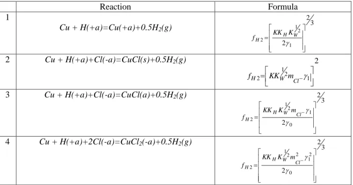
Table 5: Reactions and formula for calculating hydrogen pressure in the Cu-H-O-S-Cl system………...39

Table 6: Input material in Anoxic condition………...71

Table 7: Parameters of Dependent Components (DC, Species) at 18°C………73

Table 10: Parameters of Dependent Components (DC, Species) at 58°C………..81

Table 13: Parameters of Dependent Components (DC, Species) at 80°C………..…88

Table 14: Composition of deep granitic ground water ([35])………….………...………97

Table 18: Parameters of Dependent Components (DC, Species) at 18°C………..……..107

Table 19: Experimentally-determined composition, Eh, and pH data for the Forsmark repository ...…109

(13)

7

Executive Summary

This report addresses a central issue of the KBS-2and KBS-3 plans for the disposal of high level nuclear waste (HLNW) in Sweden; that copper metal in pure water under anoxic conditions will exist in the thermodynamically-immune state and hence will not corrode. An implied assumption in these plans is that the copper container may also be thermodynamically immune to corrosion, under certain circumstances, by virtue of the electrochemical properties of the repository near-field environment and upon the basis that native copper deposits are found in granitic geological formations around the world. However, SKB recognizes that in practical repository environments, such as that which exists at Forsmark, copper is no longer immune, because of the presence of sulfide ion, and will corrode at a rate that is controlled by the rate of transport of sulfide ion to the canister surface. This rate is estimated by SKB to be about 10 nm/year, corresponding to a loss of copper over a 100,000 year storage period of approximately 1 mm, which is well within the 5-cm corrosion allowance of the current canister design. However, it is important to note that native copper deposits have existed for geological time (presumeably, billions of years), which can only be explained if the metal has been thermodynamically more stable than any product that may form via the reaction of the metal with the environment over much of that period. Nevertheless, even the assumption of immunity of copper in pure water has been recently questioned by Swedish scientists (Hultqvist and Szakalos [1-3]), who report that copper corrodes in oxygen-free, pure water with the release of hydrogen. While this finding is controversial, it is not at odds with thermodynamics, provided that the concentration of Cu+ and the partial pressure of hydrogen are suitably low, as we demonstrate in this report. The fact that others are expereiencing difficulty in repeating these experiments may simply reflect that the initial values of [Cu+] and p_H₂ in their experiments are so high that the quantity 1/2

2 ] [Cu pH

P  is greater than the equilibrium value, Pe, as expressed in a Corrosion Domain Diagram (plots of P and Pe versus pH). Under these conditions, corrosion is thermodynamically impossible, and no hydrogen is released, because its occurrence would require a positive change in the Gibbs energy of the reaction, and the copper is therefore said to be “thermodynamically immune”. If, on the other hand, e

P

P corrosion will proceed and the value of P will rise as Cu+ and H2 accumulate at the interface. It is postulated that this condition

was met in the Hultqvist and Szakalos [1-3] experiments, thereby leading to a successful result. Eventually, however, as the corrosion products build up in the system, P increases until P = Pe and the rate of corrosion occurs under “quasi-equilibrium” conditions. Under these conditions, the reaction can occur no faster than the rate of transport of the corroding species (e.g., H+ in the reaction Cu +H+  Cu+ + 1/2H2) to, or corrosion products(Cu+, H2) from, the copper surface.

These rates may be sufficiently low that the assumption of immunity is unnecessary to qualify copper as a suitable canister material. Thus, if the corrosion rate can be maintained at a value of less than 10-8 m/year (0.01 m/year), the canister will lose only 1 mm of metal over a one hundred thousand year storage period, which is well within the designed corrosion allowance of 5-cm. However, if the rate of transport through the bentonite buffer is, indeed, that low, then it begs the question: “Why is it necessary to use copper or would a less expensive alternative (e.g., carbon steel) suffice?”

Prior to beginning extensive calculations, it was recognized that the most deleterious species toward copper are sulfur-containing entities, such as sulfide, and various polysulfides, poly thiosulfates, and polythionates, particularly those species that readily transfer atomic sulfur

(14)

8

to a metal surface (e.g. 2Cu+S2O32-  Cu2S + SO32-). Accordingly, we performed a very

thorough literature search and successfully located extensive thermodynamic data for sulfur-containing species, primarily from studies performed in Israel, that are not contained in established databases. These data are now included in the database developed in this study.

The environment within the proposed repository is not pristine, pure water, but instead is brine containing a variety of species, including halide ions, sulfur-containing species, and iron oxidation products, as well as small amounts of hydrogen (determined to be about 10-11 M by bore-hole sampling). Some of these species are known to activate copper by forming reaction products at potentials that are more negative than in their absence, thereby leading to a much larger value for Pe. For example, in the case of sulfide, whence 2Cu+HS-  Cu2S + 1/2H2, the

value of Pe rises by more than twenty-five orders of magnitude at ambient temperature, compared with that for the formation of Cu+, for sulfide concentrations that are typical of the repository. Since sulfide species are ubiquitous in groundwater in Sweden, and elsewhere, the controversy raging around whether copper corrodes in pure water is moot, at least with regard to the isolation of High Level Nuclear Waste in Sweden. In this study, we have derived CDDs for copper in the presence of a large number of species that are known or suspected to exist in the repositories. We show that a wide variety of sulfur-containing species and non-sulfur-containing entities activate copper, thereby destroying the immunity assumed for copper in pure water. For example, in addition to the sulfide species (S2-, HS-, H2S) the polysulfides (Sx2-, x = 2 – 8),

polythionates (SxO62-) and thiosulfate (S2O32-) are all found to be powerful activators of copper.

Interestingly, the poly thiosulfates (SxO32-, x = 3 – 6) are found not to activate copper. The

reason for this unexpected result is not yet known and may require determination of electron densities on the atoms in these species, in order to resolve this issue. Chloride ion, which is also ubiquitous in groundwater systems is found to be a mild activator, but the other halide ions (F-, Br-, I-) are generally not activators, except at low pH.

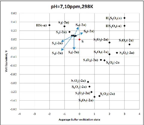
Because of their propensity to activate copper, and because some, at least, are present in the repository ground waters, sulfur species were singled out for a more intensive study. It is well-known that, except for carbon, sulfur displays the richest chemistry of any element in the periodic table. Sulfur-containing species display oxidation states ranging from -2 to +8, with a multitude of fractional oxidation states. The species are generally labile with little kinetic inhibition to interconversion. We summarize this redox chemistry in the form of volt-equivalent diagrams, in which the equilibrium potential of the species with respect to elemental sulfur multiplied by the average oxidation state of sulfur in the species is plotted against the average sulfur oxidation state for a given temperature (ranging from 25 oC to 125 oC) and pH. These diagrams provide a set of rules that indicate which pairs of species will react and which species undergo disproportionation, with the products being indicated in both instances. The diagrams have been developed to match the conditions that are found in the proposed repository. The diagrams reveal that those sulfur compounds, for example, the polythiosulfates (SxO32-, x = 3 –

6), that are found not to activate copper, are characterized by excessively low (negative) volt-equivalent values. While this is seen to be an important factor, it is not considered to be decisive and we continue with our search for a rational electrochemical thermodynamic explanation as to why the polythiosulfates (SxO32-, x = 3 – 6) are found not to activate copper. The VEDs

developed in this study represent one of the most comprehensive analyses reported to date on the redox chemistry of sulfur and provides a wealth of data for predicting the fate of sulfur in repository environments.

(15)

9

One of the surprising findings of Phase I was the non-activating behavior of S_xO₃2, x3. Thus, our preliminary explanation is that adsorption of this ion onto the metal surface occurs via the three oxygen atoms in a pyramid configuration, with the polysulfur chain extending from the apex. It is further postulated that this configuration occurrs, because of a high electron density on the oxygen atoms, compared with that of activating species, such that a partial covalent bond is formed between each oxygen atom and copper. In this configuration, it is reasoned that the sulfur atoms would not have access to the metal surface, in order to react and form Cu2S, and hence would be non-activating. Resolution of this

issue requires determination of the atomic electron densities in activating and non-activating polysulfur species and the configurations of the adsorbed species on copper. We will attempt to resolve this important issue in the next phase of this work by using Density Functional Theory to estimate atomic electron densities and to identify the most favorable configurations for the adsorbed species on copper. An important goal will be to explain why thiosulfate (S2O3

2-) is a powerful activator but the higher homologues are non-activating. In the thiosulfate case, it is possible that the electron densioty on the sulfur is higher than that on the oxygen and hence that the ion adsorbs in a configuration that allows the sulfur to react with the copper.

Under anoxic conditions the activation of copper produces hydrogen and the relationship between the equilibrium hydrogen pressure from the reaction and the hydrogen pressure in the repository is another indicator of whether copper will corrode. Thus, if the equilibrium hydrogen pressure for a reaction is greater than the hydrogen pressure in the repository, the reaction will proceed in the forward (hydrogen-producing and corrosion) direction, whereas if the equilibrium hydrogen pressure is less than that of the repository the reaction is spontaneous in the reverse direction. It is this latter situation that represents immunity to corrosion. Not unexpectedly, the results of this analysis are in accord with the findings from the Corrosion Domain Diagrams, and, again, the propensity of the sulfur-containing species to activate copper is demonstrated. Chloride ion is, again, found to be a weak activator in accordance with the CDDs. This work was also performed to more closely define the conditions of the Szakalos and Hultqvist [1-3] experiments, which have detected the formation of hydrogen when copper is in contact with highly pure, deoxygenated water. As with the CDDs, the hydrogen pressure calculations predict that the reaction of copper with water under these conditions is only spontaneous if the pressure of hydrogen and the concentration (activity) of Cu+ are both exceptionally low, providing further corroboration that the lack of agreement between the various sets of experiments reflects differences in the initial states of the experiment with respect to the quantity 1/2

2 ] [Cu pH P 

compared to the equilibrium value, Pe. In carrying out this analysis, it was necessary to consider the processes that might establish the hydrogen partial pressure in the repository. From a review of the geochemical literature, it appears that the hydrogen partial pressure is established by the hydrolysis of Fayalite [3Fe₂SiO₄2H₂O2Fe₃O₄3SiO₂2H₂] and/or the Schikorr reaction [3Fe(OH)₂Fe₃O₄2H₂OH₂]. We carried out a thermodynamic analysis of these reactions and found that the Fayalite hydrolysis reaction is, theoretically, capable of producing only a fraction of an atmosphere of H2, while the Schikorr reaction is predicted to produce an

equilibrium hydrogen pressure of the order of 1000 atm. Realization of this pressure would require that Fe(OH)2 and/or Fe2SiO4 and the reaction products (Fe3O4 and SiO2) be represent in the system. However, if Fe(OH)2 and Fe2SiO4 are minor components of the rock, they will be quickly depleted and, recognizing that hydrogen is continually lost from the system, the hydrogen concentration will be much lower than that indicated by thermodynamic calculation, which assumes a closed system. This expectation is in keeping withthe measured concentration of hydrogen from bore-hole sampling programs at Forsmark and elsewhere, which show that the

(16)

10

H2 concentration is of the order of 10-11 M, corresponding to a partial pressure of about 10-14 atm.

This low concentration, compared with the thermodynamically predicted value, indicates that the rate of loss of hydrogen from the geological formation is much greater than the rate of generation. However, it is important to recognize that sampling indicates a wide range of hydrogen concentration, with values ranging up to 10-6 M. This figure is still so much lower than the thermodynamic predictions that it raises the question as to whether the measured values are accurate or whether neither of the two reactions identified above actually occur in the repository. Certainly, if the Schikorr reaction controls the hydrogen pressure in geological formations, explaining the existence of native copper is straight forward, provided sulfur-containing species that can activate copper are are at a suitably low concentration. Even if Fayalite hydrolysis is the operative hydrogen-control mechanism, the existence of native copper is, again, readily explained, but it requires a correspondingly lower (by a factor of about 104) sulfide concentration than in the Schikorr reaction case. The discrepancy between the calculated hydrogen pressure and that sampled from bore-holes is disturbing and needs to be resolved, in spite of this issue being studied extensively by SKB (SKB R-08-85). Resolution of this issue is necessary, because hydrogen has a huge impact on the redox potential of the repository and hence upon the corrosion properties of the canisters. An accurate prediction of the evolution of corrosion damage along the Corrosion Evolutionary Path (CEP) will require accurate estimation of hydrogen fugacity in the repository over at least one hundered thousand years after it has been closed.

Currently, there exist data on the chemical composition of the ground water that are the result of analyzing “grab” samples from bore holes. While this procedure is notoriously unreliable, particularly when volatile gases are involved, it does provide good measures of dissolved components, provided that precipitation does not occur during the sampling process. Frequently, solid phases will precipitate in response to the loss of volatile gases, and unless the sampling capsule is tightly sealed considerable error may ensue. Given these caveats, as well as the fact that some of the techniques measure the total concentration of a element (e.g., sulfur as sulfate by oxidizing all sulfur species in the system to SO42- with a strong oxidizing agent, such

as H2O2), we accept the analysis of the concentrations of the ionic species, because they are

measured using the normally reliable method of ion chromatography. However, these anions (e.g., Cl-, Br-, CO32-, etc) are generally not particularly strong activators and hence are of only

secondary interest in determining the corrosion behavior of copper. Accordingly, we decided to employ a modern, sophisticated Gibbs Energy Minimization algorithm to predict the composition of the repository environment, as a function of temperature and redox condition, with the latter being adjusted by changing the relative concentrations of hydrogen and oxygen inputs to the code, in order to obtain the desired outputs. Note that the input concentrations are much greater than the output concentrations, because these gases react with components in the system as the system comes to equilibrium. After evaluating several codes, we chose GEMS, which was developed in Switzerland by Prof. Dmitrii Kulik. This code is designed specifically to model complex geochemical systems, contains a large database of compounds, and is in general use in the geochemical community. Prior to using the code to model the repository, we upgraded the database by adding thermodynamic data for various polysulfur species (polysulfides, polythiosulfates, and polythionates) that had been developed earlier in this program. However, the code became ill-behaved when the data for SxO32-, x = 3 – 7 was added.

Consultation with the code developer, Prof. Dmitrii Kulik of the Paul Scherer Institute in Switzerland failed to identify and isolate the problem and, accordingly, it was necessary to

(17)

11

remove those species from the database. The reader will recall that these are the very species that, anomalously, do not activate copper. With the code in its present form, we have modeled the repository under both oxic and anoxic conditions with the greatest emphasis being placed on the latter, because the great fraction of the storage time is under anoxic conditions. The most important finding to date is that the concentrations of the polysulfur species (polysulfides, polythiosulfates, and polythionates) under anoxic conditions are predicted to be very low, but it is still not possible, because of the uncertainty in the calculations, to ascertain with unequivocally whether these species will activate copper in the repository. However, the point may be moot, because sulfide species (S2-, HS-, and H2S) are predicted to be present in sufficient concentration

to activate copper and cause the metal to corrode under simulated repository conditions.

Finally, we have initiated work to define the corrosion evolutionary path (CEP) in preparation for modeling the corrosion of the canisters in the next phase of this program. The task of defining the CEP essentially involves predicting the redox potential (Eh), pH, and granitic

groundwater composition, as defined by the variation of temperature (note that the temperature decreases roughly exponentially with time, due to radioactive decay of the short-lived isotopes), and then applying Gibbs energy minimization to predict speciation at selected times along the path. At each step, the CDD for copper is derived and the value of P is compared to Pe to ascertain whether copper is active or thermodynamically immune. Although the polysulfur species (e.g., HS2- and S22-) are generally predicted to be present at very low concentrations, or

are predicted to be absent altogether (e.g., polysulfuroxyanions), some are predicted to be present at sufficient concentration (e.g., S22-) that they might activate copper. Thus, in the case of S22-,

the CDDs indicate that this species need be present at only miniscule concentrations (10-44 M) for activation to occur. In any event, as noted above, sulfide (H2S, HS-, and/or S2-) are predicted

to be present during the entire anoxic period at sufficiently high concentrations to activate copper, so that activation by the polysulfur species seemingly is not an important issue.

The assumption that copper is unwquivocally immune in pure water under anoxic conditions is strictly untenable, and it is even more so in the presence of activating species, such as sulfide. Thus, it appears that two conditions must be met in order to explain the existence of the native deposits of copper that occur in granitic formations: (1) A suitably high hydrogen fugacity (partial pressure) and; (2) A suitably high cuprous ion activity, as shown in this report. Accordingly, the success of the KBS-3 program must rely upon the multiple barriers being sufficiently impervious to the transport of activating species and corrosion products that the corrosion rate is reduced to an acceptable level.

(18)

12

I. Introduction

Sweden’s KBS-3 plan for the disposal of high level nuclear waste (HLNW) is partly predicated upon the assumption that copper, the material from which the canisters will be fabricated, was thermodynamically immune to corrosion when in contact with pure water under anoxic conditions. In other words, copper was classified as being a noble metal like gold. In the immune state, corrosion cannot occur, because any oxidation process of the copper is characterized by a positive change in the Gibbs energy, rather than a negative change demanded by the Second Law of Thermodynamics for a spontaneous process. Accordingly, “immunity” is a thermodynamic state that must be characterized upon the basis of thermodynamic arguments. This immunity postulate was apparently intriguing, because of the occurrence of deposits of native (metallic) copper in various geological formations throughout the World (e.g., in the upper Michigan peninsular in the USA, and in Sweden). Accordingly, it was reasoned that, during the anoxic period, when all of the oxygen that was present during the initial oxic period, due to exposure to air upon placement of the waste, had been consumed and the redox potential, Eh, had

fallen to a sufficiently low value, copper might become thermodynamically immune and corrosion might not occur, even over geological times, provided the environment remained conducive to that condition. We now understand that this condition can be realized only if hydrogen is present at a suitably high fugacity, if activating species, such as sulfide, are present at suitably low concentrations, and if the activity of Cu+ is suitably high. We also understand that these conditions cannot be met in any practical repository environment, particularly with regard to the concentrations of activating species. In that case, the corrosion of copper is thermodynamically spontaneous and the safe iosolation of HLNW requires inhibiting corrosion to the extent that the waste will be safely contained over the designated storage period.

The issue of copper immunity in pure water under anoxic conditions has developed into one of considerable controversy within both the scientific and lay communities in Sweden, because direct experimentation has failed to achieve resolution. Thus, experiments by Hultqvist, et. al. [1-3] have reported detection of hydrogen evolution when copper metal is exposed to deoxygenated, pure water, while other experiments appear to refute those claims [4-6]. The experiments were all carried out to the highest of scientific standards using hydrogen detection techniques that were more than adequate for the task of quantitatively detecting and measuring the gas, and each group reports internally-consistent results that, nevertheless, appear to be diametrically opposite from one group to the other. While the work reported in Refs. 1 to 6 is of great scientific interest, it is perhaps moot, when viewed in light of the environment that is present at Forsmark, the site of the initial HLNW repository in Sweden. Nevertheless, resolution of the scientific controversy underlying the experiments of Hultqvist,, et.al. [1-3], and those in refute, is important, because it would remove one aspect of uncertainty in the assessment of the KBS-3 plan for storing High Level Nuclear Waste (HLNW) in Sweden.

In this study, we report a comprehensive thermodynamic study of copper in contact with anoxic pure water and granitic groundwater of the type and composition that is expected in the Forsmark repository in Sweden. Our primary objective was to ascertain whether copper would exist in the thermodynamically immune state, when in contact with pure water under anoxic conditions, and to provide a thermodynamic basis for assessing the corrosion behavior of copper in the repository. In spite of the fact that metallic copper is known to exist for geological times in granitic, geological formations, copper is well-known to be activated from the immune state, and to corrode, by specific species that may exist in the environment. The principal activator of

(19)

13

copper is known to be sulfur in its various forms, including sulfide (H2S, HS-, S2-), polysulfide

(H2Sx, HSx-, Sx2-), poly sulfurthiosulfate (SxO32-), and polythionates (SxO62-). A comprehensive

study of this aspect of copper chemistry has never been reported, and yet an understanding of this issue is vital for assessing whether copper is a suitable material for fabricating canisters for the disposal of HLNW. Our study identifies and explores those species that activate copper; these species include sulfur-containing entities as well as other, non-sulfur species that may be present in the repository. In order to explore these issues, we have introduced new, innovative techniques, such as corrosion domain diagrams (CDDs) and Volt-Equivalent Diagrams (VEDs), as well as traditional Gibbs energy minimization algorithms, in order to display the chemical implications of copper activation and the electrochemical properties of the activating species, in a manner that allows a reader to discern the issues and follow their resolution. No new experiments are performed, but considerable analysis of the thermodynamic data for copper metal in contact with the environments of interested is reported. From this analysis the question of copper corrosion in pure water under anoxic conditions and in HLNW repositories is readily addressed.

II. Thermodynamic Data for Copper and Sulfur Species

The initial task in the present investigation was to review various databases and the literature for thermodynamic data. Of particular interest was assessing the consistency of the data from one database to another. High consistency was expected, because the Gibbs energies of formation, the third law entropies, and the heat capacity are commonly taken from a common source. Of course, that does not ensure accuracy, because the original measurements themselves may have been in error. A better assessment method is to compare predicted phenomena with direct experiment, by first making sure that the phenomenon that is being predicted was not used for the original derivation of the data. For example, common comparisons include calculated and observed solubility, acid/base dissociation constants, volatility, and electrode potentials. However, doing this effectively for all of the species in the database is an enormous task that is well beyond the scope of the present study. Instead, this approach is being used to assess the data for only those species for which we have doubts of appropriate accuracy. Since this task is on-going, the final results will be reported in a later report.

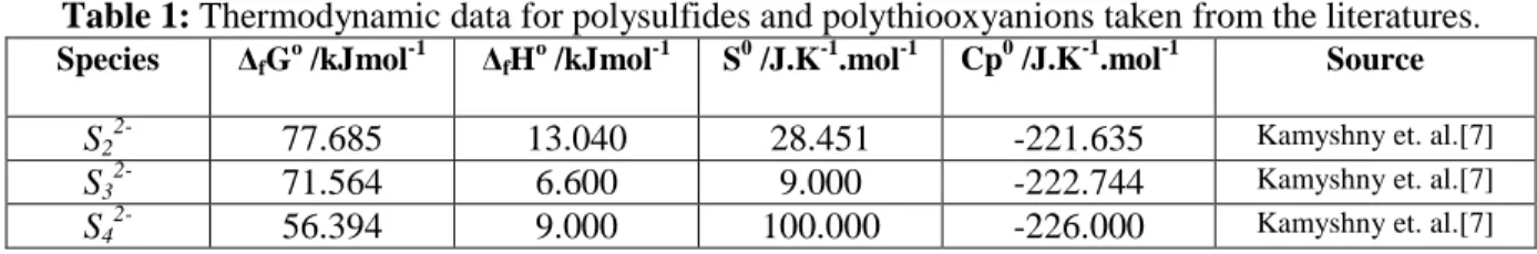
The second objective of this task was to develop a more comprehensive database for the polysulfide and polythiooxyanions by carefully reviewing the more recent literature than that included in the older databases. This proved to be highly fruitful and successful, as we were able to locate several recent papers that reported thermodynamic data for a variety of partially oxidized/reduced sulfur species, including the polysulfides, polythiosulfates, and the polythionates (Table 1). To our knowledge, Table 1 represents the most comprehensive compilation of thermodynamic data for sulfur-containing species. Even so, and recognizing the complexity of the S-O-H system, the database is far from complete, particularly with respect to the acid species.

Table 1: Thermodynamic data for polysulfides and polythiooxyanions taken from the literatures.

Species ΔfGo /kJmol-1 ΔfHo /kJmol-1 S0 /J.K-1.mol-1 Cp0 /J.K-1.mol-1 Source S2

2-77.685 13.040 28.451 -221.635 Kamyshny et. al.[7]

S3

2-71.564 6.600 9.000 -222.744 Kamyshny et. al.[7]

S4

2-56.394 9.000 100.000 -226.000 Kamyshny et. al.[7]

(20)

14

S5

2-66.666 21.338 139.000 -227.395 Kamyshny et. al.[7]

S6

2-68.189 13.300 139.000 -227.395 Kamyshny et. al.[7]

S7

2-80.951 16.500 139.000 -227.395 Kamyshny et. al.[7]

S8

2-88.272 23.800 171.000 -228.540 Kamyshny et. al.[7]

S2- 85.973 33.095 -14.602 -137.154 NBS[4], Helgeson[13] S2O3 2--518.646 -648.52 66.944 -237.631 Shock[8], NBS[10] S4O6 2--1040.253 -1224.238 257.316 -109.153 Shock[9], NBS[10] S2O4 2--600.567 -753.538 92.048 -207.684 Shock[9], NBS[10] S2O5 2--790.876 -970.688 104.600 -200.199 Shock[9], Kivialo[15] S2O6 2--969.037 -1173.194 125.520 -187.730 Shock[9], Kivialo[15] S2O7 2--795.090 -1011.101 188.334 -75.969 Williamson[11] S2O8 2--1114.868 -1344.763 244.346 -103.318 Shock[8], NBS[10] S3O32- -827.187 -951.400 118.001 -198.747 Williamson[11] S3O6 2--957.360 -1167.336 138.072 -180.243 Shock[9], Kivialo[15], Rossini[16] S4O3 2--957.384 -1085.099 138.323 -163.272 Williamson[11] S5O3 2--1030.080 -1159.700 164.004 -118.441 Williamson[11] S5O6 2--955.337 -1175.704 167.360 -162.782 Shock[9], Kivialo[15] S6O3 2--1074.377 -1205.201 192.037 -69.505 Williamson[11] S6O6 2--1196.975 -1381.000 321.323 156.185 Williamson[11] S7O3 2--1104.774 -1236.401 221.413 -18.224 Williamson[11] HS- 12.082 -16.108 68.199 -93.618 Shock[8], NBS[10], Helgeson[13] HS2 -11.506 -267.902 -742.317 -195.115 Williamson[11] HS3 -20.510 -352.402 -1023.862 -185.042 Williamson[11] HS4 -27.714 -394.401 -1156.822 -180.285 Williamson[11] HS5 -33.017 -419.601 -1227.058 -177.772 Williamson[11] HS6 -36.228 -436.299 -1261.765 -176.530 Williamson[11] H2S(a) -28.6 -39.706 125.5 183.667 Plyasunov[14] H2S2O4(a) -616.66 -733.455 213.384 155.905 Shock[9] HS2O4 --614.471 -749.354 152.716 56.282 Shock[9], Williamson[11] H2SO3(a) -537.86 -608.898 232.212 0.000 NBS[10] H2S2O3(a) -535.576 -629.274 188.280 114.724 Shock[9] HSO3- -527.613 -626.219 139.746 -5.304 Shock[8], NBS[10] H2SO4(a) -744.526 -909.392 20.083 -176.410 NBS[10] HSO4 --755.67 -889.1 125.52 22.589 Shock[8], NBS[10] HSO5 --637.440 -775.630 212.129 154.047 Shock[9] HS2O3- -532.132 -643.918 127.612 15.095 Shock[9] SO3 2--486.546 -635.55 -29.288 -280.022 Shock[9], Phillips[12] SO4 2--744.361 -909.602 18.828 -264.944 Shock[8], NBS[10] SO2(a) -300.555 -323.005 161.921 311.612 NBS[10], Shock[8] SO3(a) -525.637 -635.591 -28.995 0.000 NBS[10] HS2O5 --998.490 -1218.799 -31.229 -532.911 Williamson[11] HS2O6 --1073.389 -739.798 1929.134 6013.290 Williamson[11] HS2O7 --1372.589 -1253.798 1311.266 3950.056 Williamson[11] HS2O8 --1510.289 -1253.798 1875.687 5834.817 Williamson[11] HS3O3 --471.386 -718.899 -295.549 -1415.549 Williamson[11] HS4O3 --477.382 -760.898 -384.233 -1711.690 Williamson[11] HS5O3 --480.179 -786.098 -427.308 -1855.527 Williamson[11] SSM 2011:09

(21)

15 HS6O3 --481.378 -802.801 -447.236 -1922.074 Williamson[11] HS7O3 --481.974 -815.001 -454.085 -1944.945 Williamson[11]

III. Corrosion Domain Diagrams

The objective of deriving Corrosion Domain Diagrams is to present the consequences of the Second Law of Thermodynamics in the clearest form possible, when assessing the immunity and activation of copper. Traditionally, this subject has been addressed using potential-pH (or Pourbaix) diagrams, but this form of presentation fails to emphasize the importance of species at very low concentrations and the impact that they may have in determining the thermodynamic properties of ametal. We stress, however, that all forms of presentation essentially employ the same thermodynamic data, so that the message that needs to be relayed is in the very form of the presentation itself. In order to illustrate this feature, we need to explore the derivation of Corrosion Domain Diagrams (CDDs).

Consider the most basic corrosion reaction in the copper/water system:

Cu + H+ = Cu+ + 1/2H2 (1)

The change in Gibbs energy for this reaction can be written as ) / log( 303 . 2 12 0 2      G G RT f_H a_Cu a_H (2)

which, upon rearrangement yields

pH RT 303 . 2 G G ) a f log( 0 2 1 H2 Cu       (3)

where G0 is the change in standard Gibbs energy; i.e., the change in Gibbs energy when all components of the reaction are in their standard state with the fugacity of hydrogen,

2

H

f , and the activity of cuprous ion, a_Cu, being equal to one. At equilibrium, G0, and designating the

equilibrium values of 2

H

f and a_Cu with superscripts “e” we may write

             pH RT 303 . 2 G e Cu 2 1 , e H e 0 2 a 10 f P  (4) where Pe is termed the “partial equilibrium reaction quotient”. We now define the partial reaction quotients, P, for non-equilibrium conditions as follows

  f a_Cu P H 2 1 2 (5)

The condition for spontaneity of Reaction (1) then becomes P < Pe and immunity is indicated by P > Pe.

(22)

16

Below, we present various CDDs for the Cu-O-S-H system, in order to display the power of the method for addressing the immunity issue and for identifying those species that will activate copper. Other CDDs for wide ranges of conditions and species are given in Appendix 1. In the first instance, we consider the CDD for copper in contact with pure water under anoxic conditions (Figure 1).

Figure 1 is missing.

Figure 1: Corrosion domain diagram for copper in water as a function of

temperature.

The quantity Pe has been calculated for Reaction (1) using Equation (4) and is plotted as a function of pH in Figure 1. These plots divide the log(P) versus pH domain into regions of immunity (upper region) and corrosion (lower region), with the regions being separated by Log(Pe) versus pH for different temperatures. These plots clearly demonstrate that whether copper is immune (thermodynamically stable) depends sensitively upon the value of P, which is a property of the environment (  _Cu

2 / 1 H a f P

2 ), and hence upon the initial conditions in the system (fugacity of hydrogen and activity of Cu+). Thus, if P is small (e.g., at Point a, Figure 1), P < Pe and the corrosion of copper is spontaneous as written in Equation (1). On the other hand, if the system is located at Point (b), Figure 1), because the initial value of _Cu

2 / 1 H a f 2 is sufficiently high, P > Pe and corrosion is not possible, thermodynamically, and hence the metal is “immune”. Returning now to the case described by Point a, we note that as the corrosion reaction proceeds, the concentration of Cu+ and the fugacity of hydrogen at the interface will increase, particularly in a medium of restricted mass transport (e.g., in the bentonite buffer surrounding a canister), such that P will steadily increase with time until it meets the value of Pe at the corresponding temperature. At this point, the metal may be classified as being “quasi-immune”; “quasi” only because transport of Cu+ and H2 away from the canister surface, through the bentonite buffer

must be matched by corrosion, in order to maintain P = Pe at the metal surface. Accordingly, the corrosion rate ultimately becomes controlled by the diffusion of Cu+, H+, and H2 (in this case)

through the adjacent bentonite buffer. Thus, we conclude that, for any system starting at a point below the Pe versus pH for the relevant temperature, copper metal is not thermodynamically immune and will corrode in the repository at a rate that is governed by the rate of transport of the reactants (H+) to, and the corrosion products away from, the metal surface. Of course, this rate is

1/T /K^-1 vs Log(K) pH 0 5 10 15 20 L o g (P) -30 -25 -20 -15 -10 -5 0 273.15 433.15 333.15 Corrosion Possible

Corrosion Not Possible

Temperature /K

Pe

a

b

(23)

17

readily predicted by solving the mass transport equations for the system, if the diffusivities of Cu+ and H2 in bentonite are known. Note that a system can never cross from the corrosion

region to the immune region spontaneously as the change in Gibbs energy would become positive. That transition can be affected, however, by imposing a higher value of 

Cu 2 / 1 H a f 2 by the

addition of hydrogen and/or Cu+; this is equivalent to performing work, which is the condition for reversing an irreversible process (the “refrigerator principle”).

As noted above, for any system whose initial conditions (value of P) lie above the relevant Pe versus pH line, copper is unequivocally immune and corrosion cannot occur, as corrosion would violate the Second Law of Thermodynamics. However, it is evident, that the conditions for immunity might be engineered in advance by doping the bentonite with a Cu(I) salt and a suitable reducing agent to simulate the reducing power of hydrogen, such that the initial conditions lie above Pe versus pH. It is suggested that cuprous sulfite, Cu2SO3, might be a

suitable material, with the cation providing the suitably high Cu+ activity and the anion establishing the required reducing conditions that, otherwise, would be established by hydrogen. Of course, the dopant will slowly diffuse out of the bentonite and into the external environment, but it is expected to be sufficiently slow that the conditions of immunity may be maintained for a considerable period. Thus, in a “back-of-the-envelope” calculation,

D L

t  2/ (7)

we choose L = 10 cm and D = 10-9 cm2/s to yield a diffusion time of 1011 seconds or 316,456 years, considerably longer than the generally recognized storage horizon of 100,000 yesrs. At a time of this order, the value of P at the canister surface will have been reduced to Pe and corrosion will have initiated at a rate that is determined by the transport of reactants and products through the bentonite buffer. It is important to note that the above calculation is only a rough estimate and that a more accurate value can be obtained by solving the transport equation with experimentally determined values for the diffusivities of the reactants and products. The important point is that immunity may be maintained for a sufficiently long period that the more active components of the HLNW will have decayed away and will no longer represent a threat to the biosphere.

The analysis presented above is largely predicated on the corrosion of copper in contact with pure water (Figure 1). However, groundwater is far from pure, and a common contaminant is sulfide as H2S, HS-, or S2-. Sulfide species arises from dissolution of sulfur-containing

minerals in the host rock of the repository, from dissolution of pyrite in the bentonite, from the decomposition of organic (plant) material, and even from the action of sulfate-reducing bacteria (SRBs). It is fair to conclude that sulfide, and other sulfur-containing species are ubiquitous in groundwater environments at concentration ranging up to a few ppm, at least. It is also well-known that sulfide species (H2S, HS-, or S2-) activate copper by giving rise to the formation of

Cu2S at potentials that are significantly more negative than the potential for the formation of

Cu2O or Cu+ from water. Thus, in the presence of bisulfide, the lowest corrosion reaction of

copper may be written as:

2Cu + HS- + H+ = Cu2S + H2 (g) (8)

for which the change in Gibbs energy is written as

) a a / f log( RT 303 . 2 G G H _H 0 HS 2       (9) SSM 2011:09

(24)

18

As before, we define an equilibrium value of P and Pe as

) a / f P H₂ _HS and P f /a ) e HS e H e 2   (10) where             pH RT 303 . 2 G e HS e H 0 2 /a 10 f  (11)

The value of P under non-equilibrium conditions is simply P f /a_HS, where

2

H

f is the actual fugacity of hydrogen and a_HS is the actual activity of HS

in the repository environment.

Values of Pe versus pH are plotted in Figure 2 as a function of temperature for temperatures ranging from 0 oC to 160 oC in steps of 20 oC. Again, Pe versus pH divides the diagram into two regions corresponding to spontaneous corrosion (lower region) and immunity (upper region). The reader will note that the Pe values for the lines are more positive than those for the Cu – pure water case by a factor of about 1025, demonstrating that immunity is much more difficult to achieve in the presence of bisulfide.

Figure 2 is missing.

Figure 2: Corrosion domain diagram for copper in water + HS- as a function of temperature.

In order to illustrate the difficulties posed by small amounts of sulfide species in the environment, we note that if [HS-] = 10-12 M (3.310-8 ppm) and pH2 = 10-6 atm (0.02 ppb), the

environment is characterized by a log (P) value of -10.854, which lies well below Pe in Figure 2. Note that the range of P indicated in Figure 3 corresponds to ranges in

2 H f of 7.0610-11 to 7.0510-17 pH 0 5 10 15 20 L o g (P) -5 0 5 10 15 20 Temperature / K 273.15 433.15 333.15

Corrosion Possible (Active)

Corrosion Not Possible (Immunity)

Pe

(25)

19 atm and in 

3 S

a is calculated based on the concentration of SO42-of 38.3 to 547 mg/L that are believed to describe the variability of the environment, based upon data from Forsmark [31]. Accordingly, under these conditions, copper will corrode and hence cannot be considered to be immune. Noting again that immunity is achieved only if P > Pe, we emphasize, again, that the desired immune condition could only be achieved by having extraordinarily low concentrations of HS- and/or extraordinarily high partial pressures of hydrogen. For example, the following two sets of conditions are predicted to yield immunity, [HS-] and

2

H

p combinations of 3.3 x10-10 ppm and 10-6 atm (about a factor of 108 greater than the actual value from Forsmark) and 0.033 ppm and 1010 atm, respectively. In the first case, the concentration of HS- is orders of magnitude lower than the sulfide concentration in ground water (a few ppb to a few ppm), particularly in the presence of bentonite, which commonly contains pyrite, FeS2, and hence is an unrealistic

scenario. In the second case, the required partial pressure of hydrogen (1010 atm) is impossibly high to be achieved and maintained practically in the repository, and hence is also unrealistic. Accordingly, the prospects for achieving immunity of copper in a repository in which the ground water contains a significant concentration of sulfide species must be judged as being remote or even non-existent, at least in terms of the ground water environment that is naturally present in the system. Of course, these thermodynamic predictions can be easily checked by experiment, and experiments to do so should be performed at the earliest opportunity.

Let us now explore the feasibility of engineering the near field environment to induce immunity by the addition of CuSO3 to the bentonite buffer. In this “scoping” calculation, we

assume that the activity and fugacity coefficients are unity and we accept the SO32-/SO4

2-equivalent hydrogen pressure as being 5988 atm. From Figure 2, for pH = 7, we see that Pe has a value of 1010, so that the concentration of HS- must be below 20 ppb for the copper to be immune (i.e. for P > Pe). This number may be compared with the concentration of HS- modeled using a Gibbs energy minimization code from LLNL, which gives values for various boreholes ranging from (6.68 x 10-5 M to 1.27 x 10-10 M or 2200 ppb to 4.19x10-3 ppb) [21]. Actual borehole analyses yield much higher total sulfur concentrations (101 to 547 ppm), because the analytical technique oxidizes all sulfur species to SO42- prior to determining the concentration [21]. Of

course, much of the total sulfur probably existed as sulfate ion in the original grab sample. The calculated immunity value lies within the range estimated range for HS- concentration, demonstrating that theoretically, at least, it may be possible to engineer immunity of the copper by suitably modifying the composition of the buffer. The effect may be enhanced (i.e., the critical HS- concentration may be increased) by incorporating a copper salt having a more powerful reducing anion into the bentonite buffer and/or by increasing the salt loading. Thus, the strategy of engineering the redox conditions in the bentonite buffer appears to be a most promising approach.

It is likely that a great variety of partially oxidized/reduced sulfur species may exist in the repository, due to the oxidation of pyrite during the initial oxic period (first 100 years or so after resaturation of the buffer by groundwater) or due to the action of Sulfate Reducing Bacteria (SRBs) acting upon sulfate present in the groundwater or as Gypsum in the bentonite. The species produced are expected to include the polysulfides, (H2Sx, HSx-, Sx2-), polythiosulfates

(H2SxO3, HSxO3-, SxO32-), and the polythionates (H2SxO6, HSxO6-, SxO62-) amongst others.

Corrosion Domain Diagrams for copper in the presence of these species with log (P) being typical of repository conditions have been derived in this study and an example is shown in Figure 3.

(26)

20

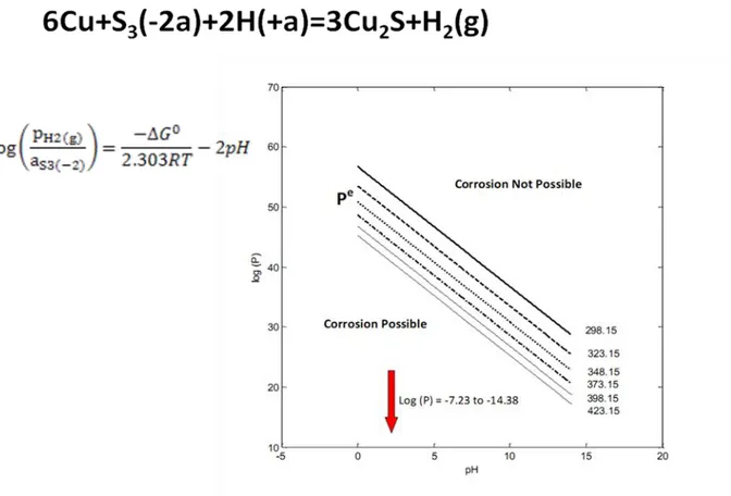
Figure 3: Corrosion Domain Diagram for copper in the presence of the

polysulfide, S32-. The red arrow indicates the range of P calculated from the

expected variability in the composion of the ground water.

Figure 4: Structure of the trithiosulfate anion. Note that the two terminal sulfur

atoms are prevented from being donated to reactive sites on a metal surface, thereby activating the metal toward corrosion, by the postulated adsorption of the species on the surface via the three oxygen atoms.

Note that log(P) for the repository, which was calculated using P f_H /a_HS

2 lies well below log(Pe) for any of the temperatures considered, and hence S32- is considered to be a

powerful activator of metallic copper. In fact, the same conclusion is arrived at for all of the

(27)

21

polysulfides (H2Sx, HSx-, Sx2-, x = 2 - 8), polythiosulfates (H2SxO3, HSxO3-, SxO32-, x = 2), and the

polythionates (H2SxO6, HSxO6-, SxO62, x = 2 - 6-), with the exception of SxO32-, x ≥ 3. Thus, the

CDD for Cu in contact with HS3O3-, Figure 5, shows that this species is a powerful activator of

copper, with the value of log(P) for the environment being estimated to be -0.47, indicating a very large driving force in terms of ΔG for the corrosion process. On the other hand, the oxyanion S3O32-, and higher members of the polythiosulfates homologous series, SxO32- (x ≥ 3),

e.g., Figure 6 and the Appendix, are predicted not to activate copper at all, as summarized in Tables 2 to 4. In these cases, the value of log(P) for the environment lies well above log(Pe) for the activating reaction. The origin of this loss in activating ability by the higher polythiosulfates remains unknown, but it is postulated to lie in the electron density on the terminal sulfur atom versus that on the three oxygen atoms (Figure 4). Thus, our preliminary explanation is that adsorption of this ion onto the metal surface occurs via the three oxygen atoms in a pyramid configuration, with the polysulfur chain extending from the apex. It is further postulated that this configuration occurrs, because of a high electron density on the oxygen atoms, compared with that of activating species, such that a partial covalent bond is formed between each oxygen atom and copper. In this configuration, it is reasoned that the sulfur atoms would not have access to the metal surface, in order to react and form Cu2S, and hence would be non-activating. Resolution of this issue requires

determination of the atomic electron densities in activating and non-activating polysulfur species and the configurations of the adsorbed species on copper. We will attempt to resolve this important issue in the next phase of this work by using Density Functional Theory to estimate atomic electron densities and to identify the most favorable configurations for the adsorbed species on copper. An important goal will be to explain why thiosulfate (S2O32-) is a powerful activator but the higher homologues are non-activating.

In the thiosulfate case, it is possible that the electron densioty on the sulfur is higher than that on the oxygen and hence that the ion adsorbs in a configuration that (a pyramid “on its side”) allows the sulfur to react with the copper. .

(28)

22

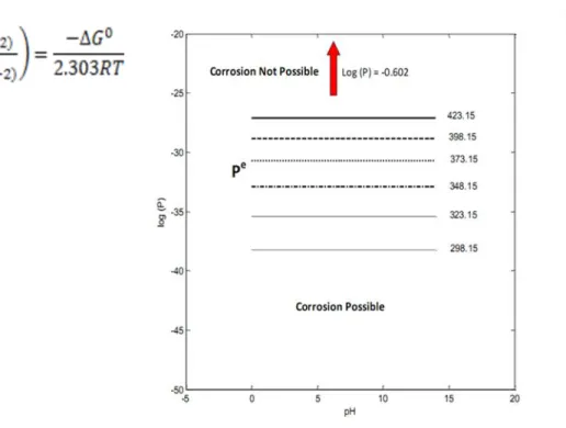
Figure 5: Corrosion Domain Diagram for copper in the presence of HS3O3-. Note

that this species is a powerful activator of copper. The red arrow indicates the range of P calculated from the documented composion of the ground water.