Multivariate Shifting Mean Plus Persistence Model for
Simulat-ing the Great Lakes Net Basin Supplies
Óli Grétar Blöndal Sveinsson1
The National Power Company (Landsvirkjun), Reykjavík Iceland Jose D. Salas
Water Resources, Hydrologic and Environmental Sciences Division, Civil Engineering De-partment, Colorado State University, Fort Collins
Abstract. The focus of this paper is to develop a multivariate model for modeling the
annual net basin supplies (NBS) of the Great Lakes. Not all NBS series show similar behavior. For example, a feature that is apparent in some but not all NBS series is a sudden shifting pattern. In this paper previous studies of univariate shifting mean models are expanded to develop multivariate contemporaneous shifting mean models. These multivariate models are further mixed with CARMA models in such a way, that the lag zero correlation in space is conserved between the underlying processes of the different models. The full contemporaneous shifting mean CARMA models are suc-cessfully applied for modeling jointly the whole Great Lakes system, preserving the spatial correlation at lag zero between different lakes, and preserving other important statistical characteristics of the individual lakes.
1. Introduction
The Great Lakes System is one of the major lake systems in the world. It involves a series of five interconnected lakes (Superior, Michigan-Huron, St. Clair, Erie, and Ontario) that are subject to inter-basin flows and net basin sup-plies (NBS). Lake St. Clair is small compared to the other four lakes but being the middle lake, it is strategically located. Lakes Superior and Ontario have been regulated for the past several decades while the intermediate lakes are not regulated, although modifications in the connecting channels have caused some effect on the lake outflows (Quinn, 1985). Regulation of the two lakes depends on the expected NBS. In addition, the regulation of Lake Ontario, be-ing the furthest downstream lake of the system, depends on the characteristics of the entire system, such as the expected NBS for all the lakes, the corre-sponding lake levels, and outflows. Thus the analysis, modeling and simula-tion of the NBS series for the various lakes have been of interest not only for testing alternative regulation plans but for re-evaluating the capacity of
1 The National Power Company
Research and Surveying Division Háaleitisbraut 68
103 Reykjavík Iceland
Tel: (+354) 515-9180 e-mail: olis@lv.is
ing waterworks, re-examining the performance of existing water systems, and assessing the capacity of new water resources systems.
Several studies have been made in the past for analyzing and modeling the NBS series of the entire Great Lakes system based on stochastic techniques. The NBS time series show complex patterns that are reflected in some of the statistical characteristics such as the mean, variance, persistence, high flow and low-flow statistics, short and long memory, and shifting level behavior – (Rassam et al., 1992). Some studies have been made attempting to understand and model some of the stochastic features of the NBS series. For example, Buchberger (1994) used a conceptual analysis based on water balance of the lakes to derive covariance properties of the annual NBS series.
Direct and indirect modeling schemes (Salas and Fernandez, 1989) have been proposed and applied for modeling monthly and quarter monthly NBS se-ries (Yevjevich, 1975; Loucks,1989; Buchberger, 1992; Rassam et al., 1992). Direct modeling schemes imply using (for instance) monthly data and building a model to simulate monthly data directly at this time scale. For example, Yevjevich (1975) used a multivariate autoregressive (AR) model after season-ally standardizing the NBS series. The drawback with this type of modeling scheme is that while the monthly statistics are generally well preserved, statis-tics at higher time scales (for example years) are generally underestimated. Likewise, other statistics related to low frequency components such as random apparent shifts in the series are not represented. On the other hand, indirect modeling schemes imply modeling and generating monthly NBS in two or more steps (stages), that is firstly the time series is modeled at a higher time scale such as years so as to reproduce key annual statistics, subsequently an-nual NBS series generated from such a model are then disaggregated into smaller time scales such as months in such a way as to reproduce monthly sta-tistics. For example, Rassam et al. (1992) employed one direct and two indi-rect modeling and generation schemes by using the so-called SPIGOT com-puter package (Grygier and Stedinger, 1990). The two indirect approaches in-cluded, a CARMA(1, 1) model with temporal disaggregation, and a mixture of multivariate AR(1) and shifting mean model with temporal disaggregation. The shifting mean model was included for generating the annual NBS series of Lakes Erie and Ontario because it was capable of reproducing the relevant sta-tistics related to lake levels and outflows better than the other alternatives. The study suggested the need of further developing multisite shifting mean models.
In this paper we develop a multivariate modeling framework using shifting mean models. Two contemporaneous models are developed, namely: the con-temporaneous shifting mean model plus AR(1) persistence dubbed as CSMAR(1) and a mixture of contemporaneous shifting mean and a contempo-raneous ARMA, dubbed CSMAR(1)-CARMA. The CSMAR(1) model is based on the single site plus persistence model, SMAR(1), suggested by Sveinsson (2006). In addition, simpler versions of the models assuming no di-rect AR(1) persistence are included. The various models are illustrated and compared using the annual NBS data of the Great Lakes system.
2. Contemporaneous SMAR(1) : CSMAR(1)
The CSMAR(1) model is a contemporaneous SMAR(1) model that can be used to model multiple time series that are correlated in space. For detailed description of the SMAR(1) model refer to Sveinsson (2002) or Sveinsson et al. (2006). If is a column vector of observations at time t for n different sites, where each site is assumed to follow a SMAR(1) process, then the CSMAR(1) process can be expressed as
[
(1) (2) (n) T t t t t = X X KX X]
t t t Y Z X = + (1)where Yt and Zt are column vectors defined in the same way as Xt. For a
sin-gle site the noise level process
{ }
Z can be written as t(2) ( ]
∑
= − = t i S S i t M I t Z i i 1 , ( ) 1Where
{ }
Mt i∞=1 ~iid N(
0,σM2 =σZ2)
, Si = N1+N2+L+Ni with , and is the indicator function equal to one if0 0 = S ) ( ) , ( t
I ab t∈(a,b) and zero otherwise. The is a discrete, stationary, delayed-renewal sequence on the positive integers, with
{ }
(Sveinsson et al., 2003 and 2005). The cross covariance function (CCVF) of {X{ }
∞ =1 i t N ) ( Geometric Positive ~ 1 iid p Nt i∞= t} at lag h is denoted by (3) ⎥ ⎥ ⎥ ⎦ ⎤ ⎢ ⎢ ⎢ ⎣ ⎡ = − − = + ) ( ) ( ) ( ) ( ] ) ( ) [( ) ( 1 1 11 T h c h c h c h c E h nn n n t h t X X X X X X X X X C L M O M L µ µwhere is the CCVF at lag h between site i and site j, and
)] ( ) [( ) ( t(i)h (Xi) t(j) (Xj) ij h E X X cX = + −µ −µ X
µ is the mean vector of Xt . In the CSMAR(1) model the
following assumptions are made about the independent sequences {Yt} and
{Zt}:
1. The sequences are modeled by a contempora-neous AR(1), CAR(1), process given by
} { , }, { }, {Yt(1) Yt(2) K Yt(n) t t t Y ε Y −µY =Φ( −1−µY)+ where is a diagonal n × n matrix, and . The CCVF of the processes in the CAR(1) model are given by
Φ {εt}~iidMVN
(
0,Cε(0))
(4) ) 1 ( ) 0 ( ) 0 ( Y TY ε C C C = −Φ (5) K , 1 , 0 ) 0 ( ) (h =Φh Y h= Y C CThus has the same decaying structure, with respect to h, in space as in time. That is, for , where is the ith row and ith column element of
) (h Y C ) 0 ( ) ( ) ( ii h ij ij h c cY = φ Y i, j∈{1,2,K,n} ii φ Φ .
2. The sequences are correlated in space only at lag zero. That is,
} { , }, { }, {Mi(1) Mi(2) K Mi(n)
(
, (0))
MVN ~ }{Mi iid 0 CM . It can be shown that a necessary and sufficient condition for {Zt} to be stationary in the
covariance is that is a common sequence for all sites. In that case the covariance function of Z
K , , 2 1 N N t at lag h is given by (6) K , 1 , 0 ) 0 ( ) 1 ( ) (h = − p h M h= Z C C
The condition that
{ }
is a common sequence for all sites may also be supported in practice, if the shifts in the means are thought of being caused by changes in natural processes, such as changes in climate. In such cases it should be expected that time series of the same hydrologic variable within a geographic region would all exhibit shifts at the same times. Thus, in general the CSMAR(1) model should not be applied for multivariate analysis of time series if it is clear that shifts in different time series do not coincide in time. Such cases can come up if a shift in a time series is caused by a construction of a dam or other man made constructions, where the construction does not affect the other time series being analyzed. Note that if M∞ =1 i t N t is assumed uncorrelated in
space then the condition for stationarity that
{ }
Nt ∞i=1 is a common sequence for all sites is not necessary any more.2.1. Parameter Estimation for the CSMAR(1) model
The parameter estimation procedure is relatively simple for the CSMAR(1) model. First the CSMAR(1) model is uncoupled into univariate SMAR(1) models. If the common p is not known, then p(i) is first estimated at each site i (Sveinsson, 2002; and Sveinsson et al., 2006). The common p can then be es-timated as a weighted average of the pˆ(i)s
∑
= + + + = n i i i n n p n n n p 1 ) ( ) ( ) ( ) 2 ( ) 1 ( ˆ 1 ˆ L (7)Given pˆthe parameters of each univariate model are reestimated.
After estimating the parameters of the univariate SMAR(1) models, what remains is estimating the non-diagonal elements of and . Using Eqs (1) and (5)-(6), and the independence of {Y
) 0 ( ε
C CM(0)
t} and {Zt} it follows that
(8) K , 1 , 0 ) 0 ( ) 1 ( ) 0 ( ) (h =Φh Y + −p h M h= X C C C
Estimates of and are obtained by solving Eq (8) with h = 0 and
h = 1 for and . It follows that
) 0 ( M C CY(0) ) 0 ( M C CY(0) (9) )) 1 ( ˆ ) 0 ( ˆ ˆ ( ] ) ˆ 1 ( ˆ [ ) 0 ( ˆ 1 X X M I C C C = Φ− −p − Φ − (10) ) 0 ( ˆ ) 0 ( ˆ ) 0 ( ˆ M X Y C C C = −
Finally using Eqs (4) and (5), Cε(0) is estimated from
(11) T T ˆ ) 0 ( ˆ ˆ ) 0 ( ˆ ) 0 ( ˆ = −Φ Φ Y Y ε C C C
It is required that and are symmetric matrixes. In order for in Eq (10) to be symmetric a complex relationship is needed between and (Sveinsson, 2002), this is unlikely to be followed by the data. Thus an adjustment is needed to make symmetric, and the simplest such adjustment is to replace all and with their respective aver-ages. If is symmetric then no further adjustment is needed in the es-timation of . ) 0 ( ˆ M C Cˆε(0) ) 0 ( ˆ M C ) 1 ( ˆij cX cˆXji(1) ) 0 ( ˆ M C ) 0 ( ˆij cM cˆMji(0) ) 0 ( ˆ M C ) 0 ( ˆ ε C
3. CSMAR(1)-CARMA(p, q)
Analyzes of multiple time series of different hydrologic variables may re-quire mixing of models. For example shifts in time series of one hydrologic variable may not be present in a time series of another hydrologic variable. Or, if different geographic locations are used for analysis of a single hydrologic variable, then characteristics of the corresponding times series may be depend-ent on their geographic location. In such cases mixing of multiple CSMAR(1) models and other time series models, such as CARMA(p, q), may be desir-able. In this section we will formulate a mixture of one CSMAR(1) model with one CARMA(p, q) model, where the lag zero cross correlation function (CCF) in space is preserved between the CARMA(p, q) model and the CAR(1) component of the CSMAR(1) model.
Lets assume that there are total of n sites, of which n1 sites follow a
CSMAR(1) model and the remaining n2 sites follow a CARMA(p, q) model.
The model of the n sites can be presented by Eq (1), where the first n1 elements
of Xt represent the CSMAR(1) model and the remaining n2 elements of Xt
rep-resent the CARMA(p, q) model
(12) ⎥ ⎥ ⎥ ⎥ ⎥ ⎥ ⎥ ⎥ ⎦ ⎤ ⎢ ⎢ ⎢ ⎢ ⎢ ⎢ ⎢ ⎢ ⎣ ⎡ + ⎥ ⎥ ⎥ ⎥ ⎥ ⎥ ⎥ ⎥ ⎦ ⎤ ⎢ ⎢ ⎢ ⎢ ⎢ ⎢ ⎢ ⎢ ⎣ ⎡ = ⎥ ⎥ ⎥ ⎥ ⎥ ⎥ ⎥ ⎥ ⎦ ⎤ ⎢ ⎢ ⎢ ⎢ ⎢ ⎢ ⎢ ⎢ ⎣ ⎡ + + 0 0 ) ( ) 1 ( ) ( ) 1 ( ) ( ) 1 ( ) ( ) 1 ( ) ( ) 1 ( 1 1 1 1 1 M M M M M M n t t n t n t n t t n t n t n t t Z Z Y Y Y Y X X X X
In general the whole vector Yt can be looked at as being modeled by a
CARMA(p, q) model (13)
∑
∑
= − = − Θ − + − Φ = − q j j t j t p j j t j t 1 1 ) (Y ε ε Y µY µYwhere {εt}~iid MVN
(
0,Cε(0))
, and the parameters Φ1,Φ2,K,Φp and are diagonal n × n matrixes. Each of the first nq
Θ Θ
Θ1, 2,K, 1 elements of Yt
is an AR(1) process, and each of the remaining n2 elements of Yt follows some
where the pi s can be different and the qi s can be different. The p and the q of
the CARMA(p, q) model are p=max(p1,p2,K,pn) and . ) , , , max(q1 q2 qn q= K
The parameter matrixes of the CARMA(p, q) are diagonal, thus estimation of parameters of the CSMAR(1)-CARMA model can be done in a similar way as for the CSMAR(1) model, where Eq (13) is uncoupled into univariate model. For the CSMAR(1) portion of Eq (13), parameters are estimated using procedures in section 2.1. For estimation of each of the univariate ARMA(pi, qi), , models refer to Salas (1993; Hipel and McLeod (1994); and Brockwell and Davis (1996). Hipel and McLeod (1994) also give a joint multivariate estimation algorithm for estimation of the parameters of the CARMA(p, q) model. The algorithm to estimate is simple, but a neces-sary condition is that the CARMA(p, q) is causal. This is equivalent to requir-ing each of the estimated univariate ARMA(p, q) models to be causal (often a common requirement in estimation procedures for ARMA models). Causality implies that Y n n n i= 1+1, 1+2,K, ) 0 ( ε C
t can be written out as an infinite moving average model. As a
result Cε(0) is estimated from
(14) T 0 ) 0 ( ) 0 ( j j j Ψ Ψ =
∑
∞ = ε Y C Cwhere are matrixes with absolutely summable elements given by and , where j Ψ I = Ψ0
∑
= Ψ Φ + Θ − = Ψ p k j k j j 1 T Ψ =0j for j < 0 and Θj =0 for j > q. For detailed information refer to Sveinsson (2002), where exact equations
are given for estimating the elements of Cε(0).
4. The Special Case : The CSM-1-CARMA Model
In the special case with φ =0 (no persistence in the Yt process) the
CSMAR(1) model in section 2 reduces to a contemporaneous SM-1 model, dubbed here as CSM-1. Thus, the sequences are cor-related in space at lag 0 only, and independent in time, with
} { , }, { }, {Yt(1) Yt(2) K Yt(n)
(
, (0) MVN ~ }{Yt iid µY CY
)
. The properties of the do not change. } { , }, { }, {Mi(1) Mi(2) K Mi(n)4.1. Parameter Estimation for the CSM-1 model
The parameter estimation procedure for the CSM-1 model follows the same steps as the parameter estimation procedure for the CSMAR(1) model in section 2.1. That is, first the CSM-1 is coupled into univariate SM-1 models and the parameters are estimated at each site using procedures in Sveinsson et al. (2006). Then the common p for all sites is estimated as a weighted average of the estimated p(i) of the univariate SM-1 models (refer to Eq (7)), and given the parameters of the univariate SM-1 models are reestimated. What re-pˆ
mains is estimating the non-diagonal elements of and . The is estimated from ) 0 ( Y C CM(0) ) 0 ( M C (15) ) 1 ( ˆ ) ˆ 1 ( ) 0 ( ˆ 1 X M C C = −p −
where if necessary is made symmetric by replacing and with their respective averages. Then is estimated from
) 0 ( M C cˆijM(0) cˆMji(0) ) 0 ( Y C (16) ) 0 ( ˆ ) 0 ( ˆ ) 0 ( ˆ M X Y C C C = −
4.2 Parameter Estimation for the CSM-1-CARMA model
The CSM-1-CARMA follows the same concept as the CSMAR(1)-CARMA model in section 3. Given the CSM-1 model then parameters of the CSM-1-CARMA model are estimated using the procedures for estimation of the CSMAR(1)-CARMA parameters in section 3, where each of the elements of {Yt} corresponding to the CSM-1 process is looked at as being modeled by
an ARMA(0, 0) process.
5. The Great Lakes System
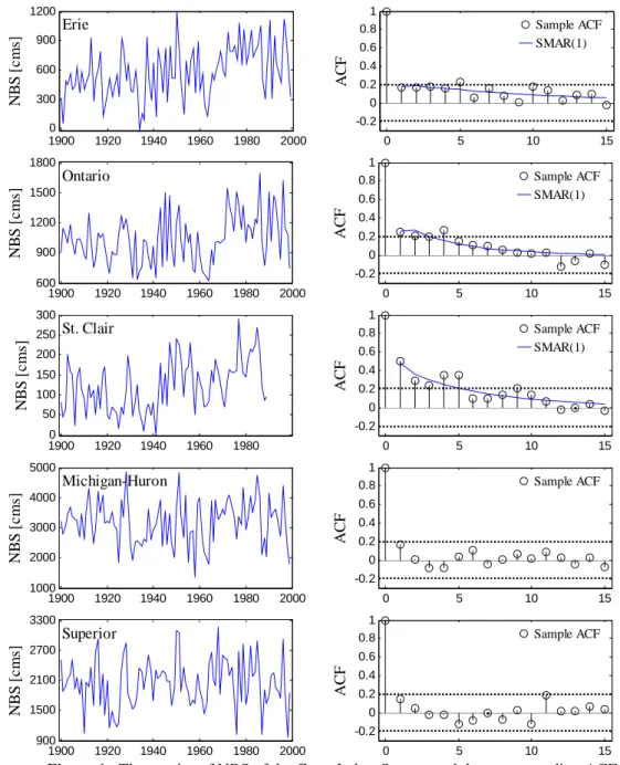
The intent here is to fit a multivariate model to the annual net basin sup-plies (NBS) of the lakes in the Great Lakes system using the procedures pre-sented in this paper. The data were obtained from Hydro-Quebec, and span the period 1900-1999 for lakes Erie, Michigan-Huron, Ontario, and Superior, and the period 1900-1989 for Lake St. Clair. Data post 1989 for Lake St. Clair were still preliminary, and hence are not used in this study. The annual NBS time series of the Great Lakes and their ACFs can be seen in Fig. 1. The data for Lake Superior and Lake Michigan-Huron in do not seem to exhibit any sudden shifts, and in addition the ACFs of the data do not have shapes that are expected of the SMAR(1) model. On the other hand, the data for the other lakes in appear to be characterized by sudden shifts. Furthermore, the cross correlation coefficients at lag zero are significant across all lakes (not shown). Thus, contemporaneous models could be used to preserve the lag zero cross correlation coefficient between different lakes.
The sample mean, standard deviation, skewness, Hurst slope K, storage ca-pacity SC, and the longest drought length DL and the corresponding drought magnitude DM based on demand level d =µˆX of the Great Lakes data are shown in Table 1.
Table 1. Sample statistics of the Great Lakes NBS time series. Fitted ACFs for the CSMAR(1) and the CSM-1 models are also shown.
Statistic Erie Ontario St. Clair Michigan-H. Superior
X µˆ [cms] 574.1 1033 121.7 3177 2043 X σˆ [cms] 265.4 241.6 63.34 737.0 478.8 X γˆ [cms] 0.138 0.491 0.311 -0.091 0.033 K 0.787 0.786 0.847 0.713 0.654 SC [cms] 5506 5083 1529 11978 4755 DL 8 11 9 8 5 DM [cms] 1720 2034 659.3 6029 3850
1900 1920 1940 1960 1980 2000 0 300 600 900 1200 Erie NB S [ c ms ] 0 5 10 15 -0.2 0 0.2 0.4 0.6 0.8 1 Sample ACF SMAR(1) AC F 1900 1920 1940 1960 1980 2000 600 900 1200 1500 1800 Ontario NB S [ c ms ] 0 5 10 15 -0.2 0 0.2 0.4 0.6 0.8 1 Sample ACF SMAR(1) ACF 1900 1920 1940 1960 1980 0 50 100 150 200 250 300 St. Clair NB S [ c ms ] 0 5 10 15 -0.2 0 0.2 0.4 0.6 0.8 1 Sample ACF SMAR(1) ACF 1900 1920 1940 1960 1980 2000 1000 2000 3000 4000 5000 Michigan-Huron NB S [ c ms ] 0 5 10 15 -0.2 0 0.2 0.4 0.6 0.8 1 Sample ACF ACF 1900 1920 1940 1960 1980 2000 900 1500 2100 2700 3300 Superior NB S [ c ms ] 0 5 10 15 -0.2 0 0.2 0.4 0.6 0.8 1 Sample ACF ACF
Figure 1. Time series of NBS of the Great Lakes System and the corresponding ACFs.
5.1 Fitting a CSMAR(1)-CARMA(p, q) model to the Great Lakes
We will attempt to fit a mixture of CSMAR(1) and a CARMA(p, q) model to the data, where the lakes Erie, Ontario, and St. Clair will be modeled by a CSMAR(1) model, and the lakes Michigan-Huron and Superior will be mod-eled by CARMA(p, q) model. The ACF and the partial ACF (not shown) of lakes Michigan-Huron and Superior in Fig. 1 suggests a CARMA(0, 0) model (a bivariate normal model) or a CARMA(1, 0) model. Lake St. Clair has 10 year shorter record than the other lakes. Thus, the models are fitted to sample series of different lengths. The approach used here preserves the variance of
the full records and the lag zero correlation between concurrent records. For further information refer to Sveinsson (2004).
For the purpose of this study a CARMA(0, 0) model was selected for mod-eling lakes Michigan-Huron and Superior. The CSMAR(1)-CARMA and the CSM(1)-CARMA models were both fitted to the data, but only the estimated parameters of the CSMAR(1)-CARMA model are shown in Table 2. The fit-ted ACFs used in parameter estimation of the univariate SMAR(1) models are shown in Fig. 1.
To analyze how capable the fitted models are in preserving the sample sta-tistics used in the fitting procedures, 1,000 realizations of the same lengths as the historical records were generated for the full models in Table 2. All the
Table 2. Parameters of the fitted CSMAR(1)-CARMA model.
Parameter Erie Ontario St. Clair Michigan-H. Superior
X ϕˆ -0.1170 -0.0162 0.1262 pˆ 0.1574 0.1574 0.1574 Y µˆ [cms] 574.1 1033 121.7 3177 2043 22401 18016 5519 ) 0 ( ˆ M C [cms] 18016 18121 3973 5519 3973 2002 48058 26654 3445 103113 37944 26654 40238 4323 114183 31060 ) 0 ( ˆ Y C [cms] 3445 4323 2010 20964 7431 103113 114183 20964 543228 195286 37944 31060 7431 195286 229280 47400 26603 3496 103113 37944 26603 40228 4331 114183 31060 ) 0 ( ˆ ε C [cms] 3496 4331 1978 20964 7431 103113 114183 20964 543228 195286 37944 31060 7431 195286 229280
lakes have historical records of the same length, n = 100, except Lake St. Clair, which has a record length n = 90. Thus the generated records for Lake St. Clair were truncated to match the length of the historical record. The average sam-ple statistics of the 1,000 generated realizations are shown in Table 3. Com-paring with the historical sample statistics in Table 1, the mean and the stan-dard deviation are well preserved for all lakes. Comparing the storage related statistics K, SC, DL, and DM in Table 3 with the corresponding historical sta-tistics in Table 1, it can be said that they are in general relatively well pre-served. Comparing the storage related statistics of the two fitted models, then the CSMAR(1)-CARMA and the CSM-1-CARMA give very similar results. A reason for the similarity may be that the φ parameters are close to zero in the CSMAR(1) part of the CSMAR(1)-CARMA model.
In Table 4 the lag 0 and lag 1 historical CCF matrixes are shown along with the corresponding CCF matrixes based on the 1,000 realizations of length
n. Comparing the CCF matrixes based on the generated sequences with the
historical CCF matrixes, then as expected the lag 0 CCF is very well preserved between all stations. The lag 1 CCF for the CSMAR(1) part of the model (the upper 3 × 3 submatrix of ρˆX(1)) may not be exactly preserved due to the ad-justments to and to make them symmetric, but in general the off-diagonal averages of and should be relatively well pre-served. The values of the lag 1 CCF in Table 4 support this. Note that any lag 1 CCF including Lake Michigan-Huron or Lake Superior is not expected to be preserved. Comparing the results among the two different models (results not shown for the CSM(1)-CARMA model), then again both models give similar results. ) 0 ( ˆ M C Cˆε(0) ) 1 ( ˆXij ρ ρˆXji(1)
Table 3. Average sample statistics of 1,000 generated NBS series of the Great Lakes of the same lengths as the historical records.
Statistic Erie Ontario St. Clair Michigan-H. Superior
CSMAR(1)–CARMA Model X µˆ [cms] 573.3 1033 121.9 3175 2042 X σˆ [cms] 261.2 237.1 61.33 732.2 474.9 X γˆ [cms] -0.014 0.006 -0.011 -0.010 0.004 K 0.727 0.730 0.779 0.616 0.617 SC [cms] 4877 4484 1290 8434 5475 DL 8.660 8.794 10.87 5.931 5.986 DM [cms] 2379 2206 760.4 4044 2624 CSM(1)–CARMA Model X µˆ [cms] 573.3 1033 121.9 3175 2041 X σˆ [cms] 261.3 237.0 61.31 732.1 474.9 X γˆ [cms] -0.013 0.008 -0.006 -0.010 0.004 K 0.728 0.729 0.779 0.616 0.617 SC [cms] 4890 4490 1300 8433 5476 DL 8.612 8.707 10.80 5.934 5.991 DM [cms] 2385 2184 752.5 4036 2624
6. Summary and Final Remarks
In this paper a multivariate shifting mean modeling framework was devel-oped. More precisely, a contemporaneous version of the univariate shifting mean autoregressive AR(1) model, SMAR(1), in Sveinsson et al. (2006), was developed and dubbed as CSMAR(1). In addition, a general contemporaneous model mixing CSMAR(1) and CARMA models was developed for modeling of systems, where some of the sites exhibit sudden shifting patterns while oth-ers do not. This model was dubbed as CSMAR(1)-CARMA. The special cases of the above models assuming no direct AR(1) persistence in the CSMAR(1) model were also developed. The special cases were, dubbed as CSM-1 and CSM-1-CARMA. A necessary condition for stationarity of the CSMAR(1) is that the sequence of the mean level lengths is common for all
sites, that is that shifts at different sites coincide in time. The above models are capable of preserving the lag zero cross correlation in space between different sites. In addition, for sites modeled by the CSMAR(1) or the CSM-1 models, some characteristics related to the lag one cross correlation in space are also preserved.
Table 4. Historical and generated cross correlation function (CCF) matrixes. The generated CCF is the average of 1,000 generated NBS series of the same lengths as the historical records.
Statistic Erie Ontario St. Clair Michigan-H. Superior Historical CCF Matrixes 1 0.697 0.549 0.527 0.299 0.697 1 0.569 0.641 0.269 ) 0 ( ˆX ρ 0.549 0.569 1 0.452 0.245 0.527 0.641 0.452 1 0.553 0.299 0.269 0.245 0.553 1 0.173 0.198 0.144 0.030 0.156 0.220 0.250 0.084 0.151 0.255 ) 1 ( ˆX ρ 0.393 0.380 0.504 0.196 0.240 0.181 0.129 0.027 0.168 0.322 0.006 -0.014 0.036 -0.066 0.153
CSMAR(1)–CARMA: average generated CCF Matrixes
1 0.692 0.521 0.536 0.301 0.692 1 0.537 0.652 0.271 ) 0 ( ˆX ρ 0.521 0.537 1 0.461 0.251 0.536 0.652 0.461 1 0.552 0.301 0.271 0.251 0.552 1 0.142 0.164 0.226 -0.065 -0.036 0.204 0.204 0.189 -0.018 -0.005 ) 1 ( ˆX ρ 0.275 0.232 0.417 0.052 0.029 -0.002 -0.004 -0.002 -0.009 0.000 -0.001 0.003 -0.001 -0.003 -0.004
Historical records of some of the lakes in the Great Lakes system show evidence of sudden shifts in addition to autocorrelation, while records for other lakes do not indicate such behavior. The proposed models, where applied for modeling jointly the Great Lakes system as a whole, with lakes Erie, Ontario, and St. Clair modeled by contemporaneous shifting mean models, and lakes Michigan-Huron and Superior modeled by a CARMA(0,0) model. The models were capable of preserving the lag zero spatial correlation between different lakes, in addition to preserving other important statistical characteristics of the individual lakes.
As a general conclusion, the proposed mixture models mixing contempora-neous shifting mean models and contemporacontempora-neous ARMA models appear to be robust and seem to have a wide range of applicability for modeling of hydro-climatic and geophysical systems.
Acknowledgements. Support from the Colorado Agricultural Experiment Station
pro-ject on ``Predictability of Extreme Hydrologic Events Related to Colorado's Agricul-ture'', National Science Foundation grant CMS-9625685 on ``Uncertainty and Risk Analysis Under Extreme Hydrologic Events'', and support from Hydro-Quebec are gratefully acknowledged.
References
Brockwell, P. J. and R. A. Davis, 1996: Introduction to Time Series and Forecasting. Springer Texts in Statistics. Springer, first edition.
Buchberger, S., 1992: Modeling and forecasting Great Lakes monthly net basin sup-plies. Technical report, U.S. Army Corps of Engineers, Detroit, MI. 48pp.
Buchberger, S., 1994: Modeling and forecasting of Great Lakes annual net basin sup-plies. Water Resources Research, 30(10):2725-2735.
Grygier, J. C. and J. R. Stedinger, 1990: SPIGOT a Synthetic Streamflow Generation Software Package, Technical Description, Version 2.6. Cornell University, Ithaca, New York.
Hipel, K. W. and A. I. McLeod, 1994: Time Series Modelling of Water Resources and Environmental Systems. Number 45 in Developments in Water Science. Elsevier, first edition.
Loucks, E., 1989: Modeling the Great Lakes Hydrologic-Hydraulic System. PhD the-sis, University of Wisconsin.
Quinn, F. H., 1985: Temporal effects of St. Clair river dredging on lakes St. Clair and Erie water levels and connecting channel flow. Journal of Great Lakes Research,
11(3):400-403.
Rassam, J.-C., Faherazzi, L. D., Bobée, B., Mathier, L., Roy, R., and L. Carballada, 1992: Beauharnois-Les Cedres spillway: Design flood study with stochastic ap-proach. Final report to the experts committee, Hydro-Québec, Montreal, Quebec, Canada. 105pp.
Salas, J. D., 1993: Analysis and Modeling of Hydrologic Time Series, chapter 19. Handbook of Hydrology. McGraw-Hill.
Sveinsson, O. G. B., 2002: Modeling of stationary and non-stationary hydrologic processes. PhD thesis, Colorado State University, Fort Collins, Co.
Sveinsson, O. G. B., 2004: Unequal record lengths in SAMS. Unpublished manu-script (please contact author).
Sveinsson, O. G. B., Salas, J. D., Boes, D. C., and R. A. Pielke Sr., 2003: Modeling the dynamics of long term variability of hydroclimatic processes. Journal of Hydrometeorology, 4:489-505.
Sveinsson, O. G. B., Salas, J. D., and D. C. Boes, 2005: Prediction of extreme events in Hydrologic Processes that exhibit abrupt shifting patterns. Journal of Hydro-logic Engineering, 10(4):315-326.
Sveinsson, O. G. B., Salas, J. D., and V. Fortin, 2006: Shifting mean plus persistence model for simulating the great lakes net basin supplies. Journal of Hydrologic Engineering, submitted.
Yevjevich, V., 1975: Generation of hydrologic samples-case study of the Great Lakes. Hydrology Paper 72, Colorado State University, Fort Collins, CO. 39pp.