Determining an optimal approach for human occupancy recognition in a study room using non-intrusive sensors and machine learning

(1)

Teknik och samhälle

Datavetenskap och medieteknik

Examensarbete

15 högskolepoäng, Bachelor Thesis

Determining an optimal approach for human occupancy

recognition in a study room using non-intrusive sensors and

machine learning.

Fastställande av ett optimalt angreppssätt för att beräkna antalet personer i ett studierum med icke-inkräktande sensorer och maskininlärning.

Lars Korduner

Mattias Sundquist

Examen: Kandidatexamen 180 hp Huvudområde: Datavetenskap Program: Systemutvecklare Datum för slutseminarium: 2018-05-24

Handledare: Agnes Tegen Examinator: Magnus Johnsson

(2)

(3)

Sammanfattning

Mänskligt igenkännande med användning av sensorer och maskininlärning är ett fält med många praktiska tillämpningar. Det finns några kommersiella produkter som på ett tillför-litligt sätt kan känna igen människor med hjälp av videokameror. Dock ger videokameror ofta en oro för inkräktning i privatlivet, men genom att läsa det relaterade arbetet kan man hävda att i vissa situationer är en videokamera inte nödvändigtvis mer tillförlitlig än billiga, icke-inkräktande sensorer. Att känna igen antalet människor i ett litet studie / kontorsrum är en sådan situation. Även om det har gjorts många framgångsrika studier för igenkänning av människor med olika sensorer och maskininlärningsalgoritmer, kvarstår en fråga om vilken kombination av sensorer och maskininlärningsalgoritmer som är allmänt bättre. Denna avhandling utgår från att testa fem lovande sensorer i kombination med sex olika maskininlärningsalgoritmer för att bestämma vilken kombination som överträf-fade resten. För att uppnå detta byggdes en arduino prototyp för att samla in och spara läsningarna från alla fem sensorer i en textfil varje sekund. Arduinon, tillsammans med sensorerna, placerades i ett litet studierum på Malmö universitet för att samla data vid två separata tillfällen medan studenterna använde rummet som vanligt. Den insamlade datan användes sedan för att träna och utvärdera fem maskininlärningsklassificerare för var och en av de möjliga kombinationerna av sensorer och maskininlärningsalgoritmer, för både igenkänningsdetektering och igenkänningsantal. I slutet av experimentet konstater-ades det att alla algoritmer kunde uppnå en precision på minst 90% med vanligtvis mer än en kombination av sensorer. Den högsta träffsäkerheten som uppnåddes var 97%.

Abstract

Human recognition with the use of sensors and machine learning is a field with many practical applications. There exists some commercial products that can reliably recognise humans with the use of video cameras. Video cameras often raises a concern about privacy though, by reading the related work one could argue that in some situations a video camera is not necessarily more reliable than low-cost, non-intrusive, ambient sensors. Human occupancy recognition in a small sized study/office room is one such situation. While there has been a lot of successful studies done on human occupancy recognition with various sensors and machine learning algorithms, a question about which combination of sensors and machine learning algorithms is more viable still remains. This thesis sets out to test five promising sensors in combination with six different machine learning algorithms to determine which combination outperformed the rest. To achieve this, an arduino prototype was built to collect and save the readings from all five sensors into a text file every second. The arduino, along with the sensors, was placed in a small study room at Malmö University to collect data on two separate occasions whilst students used the room as they would usually do. The collected data was then used to train and evaluate five machine learning classifier for each of the possible combinations of sensors and machine learning algorithms, for both occupancy detection and occupancy count. At the end of the experiment it was found that all algorithms could achieve an accuracy of at least 90% with usually more than one combination of sensors. The highest hit-rate achieved was 97%.

(4)

(5)

Acknowledgements

We would like to thank Agnes Tegen, our supervisor for helping and guiding us throughout the thesis. The students Sofie Jönsson, Jennie Neubert, Embla, Malin, Nanna, Amanda, Vanillia, Sara, Sabina, Amanda, Irma, Alexandra, Dellehaz, Emelie Grachinaj, Sofie Pers-son, Rikard Almeren, Amin Harirchian, Max Frennessen, Vedrana Zeba, Lykke Levin as well as Hanni for letting us run our experiment whilst they were studying. Maria Ko-rduner for providing us with an architectural design of the study room. And lastly the Internet of Things and People Research Center and Johan Holmberg for letting us use their prototype.

(6)

(7)

1 Introduction

1.1 Background

There is a need to be able to recognize human occupancy in a space with high accuracy and low-cost methods. There are many use-cases for human occupancy recognition. In energy consumption reduction, knowing if a space is occupied or not can be used to control ventilation and temperature systems. Human occupancy recognition data can be used to optimize room-booking systems. It can also be used for monitoring purposes, for example in medical facilities and in security systems.

One category of methods for human occupancy recognition is with the use of a super-vised machine learning model (SMLM). A SMLM is an algorithm with pattern recognition abilities that can be used for classification and regression problems. Human occupancy recognition is a classification problem that can be solved with a SMLM.

A SMLM can be built, in short, by training it with labeled data. Given enough labeled examples, the SMLM learns to recognize patterns and associate certain patterns of data with a particular label. A well-built SMLM can be given data without labels and make the correct prediction with high accuracy.

To be able to build a SMLM, data is required. It is required for training the SMLM, it is required for testing the SMLM and it is required whenever there is a need to classify new data. A SMLM that is designed to recognize human occupancy inevitably needs data which is collected from humans. This immediately raises a concern about privacy-intrusion.

Based on the related work, a strong argument can be made that intrusive data-gathering methods, such as cameras and wearable devices, does not necessarily achieve a higher accuracy than non-intrusive data-gathering methods, such as low-cost ambient sensors, in human occupancy recognition. Both Varick et al [1], which uses data from cameras, and Irvan et al [2], which uses data from non-intrusive ambient sensors, achieved a high accuracy in human occupancy recognition.

All human occupancy recognition methods that uses a SMLM requires two components: a data-gathering method and an algorithm for the SMLM. Though it is proven that non-intrusive human occupancy recognition methods can achieve a high accuracy, it is not clear which combination of data-gathering method and SMLM algorithm performs best in an equal environment.

By using five promising data-gathering methods in combination with six promising SMLM algorithms, this thesis will determine which combination of data-gathering methods and SMLM algorithms achieves the highest accuracy in a given environment.

1.2 Research aim

Earlier research such as Candanedo et al [3], Dodier et al [4] and Zhang et al [5] conducted their experiments and main focus in an office environment where occupants usually do not differ much and work is done in silence or as a meeting. Our thesis therefor aims to instead conduct our experiment in a study room at a university where there is a larger difference in occupancy and the occupants actions. To achieve this, an arduino setup, complete with a fixed set of sensors is put in a study room located in the Malmö university library shown in Figure 1. Sensory data will then be received and collected to then be inserted as data

(10)

tuples in different machine learning algorithms to determine if it is possible to achieve a high accuracy in human occupancy recognition.

In this thesis, we aim to answer the following three research questions:

1. What combination of sensors and machine learning algorithms gives the best accuracy for classifying human occupancy in a university study room?

2. What is the minimal combination of sensors and machine learning algorithms needed for 90 percent accuracy in human occupancy recognition?

3. What single sensor, if any, outperformed the rest, and what single machine learning algorithm outperformed the rest in classifying human occupancy in a room?

This will then be compared to earlier research to determine if there are any correlations between the result of our research and earlier research.

Figure 1: Depicts study room OR:B533

2 Theory

This section describes the data-gathering methods, the machine learning algorithms, the programming language and the software libraries used in this thesis.

2.1 Sensors

2.1.1 Passive infrared sensor

A Passive Infrared (PIR) sensor is an electronic sensor that can read the infrared light radiation from objects in its view. The infrared light radiation is often focused through a specially designed lens called a Fresnel lens where it hits a set of pyroelectric sensors. These pyroelectric set of sensors generates energy when exposed to the infrared light radiation. When a human walks in front of the PIR-sensor, the pyroelectric sensors will generate

(11)

energy in a certain pattern. A chip on board the PIR-sensor reads the pyroelectric energy patterns and calculates if motion has been detected or not. An analog PIR sensor outputs 0 if no motion pattern is detected and 1 if motion is detected. [6]

2.1.2 Air quality sensor

Indoor air quality can be determined by measuring the total volatile organic compound (TVOC) count in a room. VOCs are organic chemicals with a low boiling point which causes large number of molecules to evaporate and enter the surrounding air. A TVOC sensor can read the parts per million (ppm) concentration of VOCs in the air. Most scents and odors are of VOCs. Some types of VOCs can be dangerous to human health and a high enough TVOC ppm can even rapidly lead to unconsciousness or death. VOCs that are caused by humans are regulated by law, especially indoors where VOC concentrations tend to be the highest.

Indoor air quality can also be measured by calculating the carbon dioxide (CO2) count in the room. CO2 is a colorless gas which is exhaled by air-breathing land animals, includ-ing humans. [7]

2.1.3 Luminosity sensor

A luminosity sensor is used to measure the luminous flux (lux) per unit area. Lux is described as the perceived power of light. Some luminosity sensors have infrared diodes, which means that it measures light that is not visible to humans. Some luminosity sensors have full spectrum diodes, which means that it measures human-visible light and some luminosity sensors have both infrared diodes and full spectrum diodes. Different luminosity sensors also measures lux in different ranges. [8]

2.1.4 Sound sensor

A sound sensor often measures the amplitude of sound. The amplitude of sound is the maximum extent of a vibration or displacement of a sinusoidal oscillation. Although decibel is not the same as amplitude, it is strongly correlated and can be calculated by using a simple equation on the amplitude. Most sound sensors also have the capacity to output a binary indication of the presence of sound, 1 if sound has been detected and 0 if no sound has been detected. [9]

2.2 Supervised Machine Learning

A supervised machine learning model (SMLM) is an algorithm with pattern recognition abilities. A SMLM can be trained to solve classification problems and regression problems. Classification is the task of approximating a mapping function from input variables to discrete output variables. Regression is the task of approximating a mapping function from input variables to a continuous output variable.

Predicting if an image contains a cat or a dog is primarily a classification problem because the output is in the form of a discrete output variable, either a cat or a dog. The price of a used car is primarily a regression problem because the output is in the form of a continuous output variable, the predicted price of the car. Human occupancy count in

(12)

a room is primarily a classification problem where the input is data from sensors and the output is the number of human occupants in the room.

To solve any problem with a SMLM, the following steps are necessary:

1. Determine the problem and determine the data-gathering method. To solve a problem with a SMLM, information about the problem is needed. The information needs to be digital, or be transferable into digital, in the form of data points. It is important that the SMLM have a sufficient amount data points to learn from. It is also important that the data-gathering method can produce different values for different states so that the SMLM can learn to differentiate one state from another. In the case of predicting if an image contains a cat or a dog, one single image of each pet is probably not enough for the SMLM to recognize the difference between all images of cats and dogs. In the case of predicting human occupancy count in a room under normal circumstances, using only a magnetic sensor is not a good idea since humans does not affect magnetic sensors enough for them to give different readings.

2. Gather the training data.

As mentioned in step 1, the amount of gathered data points needs to be sufficient enough for the SMLM to learn from. Different types of problems requires different amounts of data points. In the case of predicting if an image contains a cat or a dog the number of ways a cat or a dog can be depicted in an image is nearly infinite. One image might be centralized on the face of a cat/dog, another image might have a cat/dog in a small part of the bottom left corner, another image might show a cat/dog that is camouflaged well with the background, and so on. In general, but especially in problems like this, more training data is better. In the case of predicting human occupancy count in a room with a single sensor the output from that sensor will be in a finite range. Even if more sensors are added then the combined output will still be in a finite range. In problems like human occupancy recognition, the amount of data points are important but the choice of sensors is perhaps equally as important.

It is also important to equalize the gathered data points so that every data point is structured the same way. In the case of predicting if an image contains a cat or a dog then each image can for example be cropped to be 200x200 pixels. Those pixels can then be flattened into a 1D-array of 40000 elements, as long as every index in the 1D-array always represents the same index in the images pixel array. In the case of predicting human occupancy count then each data point from a sensor can for example be transferred into a 1D-array, as long as each index in the 1D array always represents a certain sensor value.

Another thing to consider when using most SMLM is that they can only handle real values, such as integers of floating point values, as input as they need to perform mathematical calculations on the input as part of the learning algorithm.

3. Assign labels to the training data.

In order for a SMLM to be able to predict which label a certain data point might belong to, a label must be presented to the SMLM together with each data point

(13)

in the training stage. The labels tell the SMLM what the data represents. If step one and two is done correctly, and given enough data points with labels, the SMLM learns to recognize that certain ranges of data points belong to certain labels. In many cases, assigning labels to the training data can be, and should be, done when collecting the training data. This is because the number of data points that is collected is often a large number and reviewing the data points one-by-one to assign labels to them is a very tedious and time consuming job.

It is also important to remember that most SMLM algorithms can only deal with labels as real values, such as integers or a floating point value, and can not deal with labels as, for example, strings or characters. In the case of predicting if an image contains a cat or a dog, "0" as a label could represent that the image contains a cat and "1" as a label could represent that the image contains a dog. A simple converting algorithm can be used if the labels are stored as anything else than real values. 4. Choose an algorithm for the SMLM.

Supervised machine learning algorithms can be divided into two classes: classification algorithm and regression algorithms. Each class specializes in solving a particular problem.

Classification is the task of approximating a mapping function from input variables to discrete output variables. A binary classification problem requires the data points to be classified into one of two classes. A multi-class classification problem requires the data points to be classified into one of three or more classes. Predicting if an image contains a cat or a dog is a binary classification problem because each image can only be classified as either a cat or a dog. Predicting human occupancy count is a multi-class classification problem because each data point can be classified into one of multiple classes.

Regression is the task of approximating a mapping function from input variables to a continuous output variable. The continuous output variable in this case is a real value, such as an integer or floating point value. These are often quantities, such as amounts and sizes. A regression problem requires the prediction of a quantity. Pre-dicting used car prices is a problem that can be solved by a SMLM with a regression algorithm since the output is a continuous real value.

5. Train the SMLM.

When the problem has been determined, the data has been collected, labels has been assigned to the data points and an algorithm has been chosen for the SMLM then the training of the SMLM can begin. The training step is one of the more automatic steps in building an SMLM since all of the work is done by the computer that is running the SMLM algorithm. This, however, does not mean that it is the quickest step. Training an algorithm can sometimes take hours, days or even weeks to complete. The time it takes to train a SMLM depends primarily on three factors: the amount of training data, the choice of algorithm and the hardware of the computer being used to train the SMLM.

In the case of the amount of training data, it is not as simple as saying that the amount of training data scales linearly, that less amount of training data is faster

(14)

and that more amount of training data takes longer time. Estimating the right amount of training data is difficult because there is no metric that quantifies the amount of training data related to the performance of the model. The Dota team from OpenAI [10] proposes a new statistical metric that effectively predicts the right amount of training data to use to train specific deep learning models.

In the case of the hardware of the computer that is being used to train the SMLM, it is generally the case that more is better. A high performance GPU that is capable of calculating advanced mathematical equations at high speed is better than a low performance GPU. This generally also holds true for other hardware components such as the CPU and the RAM.

6. Evaluate the accuracy of the SMLM.

Many SMLMs can give an indication of how well it performed in the training phase but in order to evaluate the accuracy of the SMLM it has to be tested on data. The data cannot already have been used in training and cannot have an attached label. It is important that the testing data is structured exactly the same as the training data is structured. It is also important that, even though the testing data set is often much smaller than the training data set, the testing data sample is representative of all of the training data. It is often a good idea to gather enough data points in step 2 so that the data set can be split into both training and testing data. This is done both to save time but it is also done to not affect any variables in the data that might be subject to change if collected at separate dates.

When the testing data is collected then accuracy is simply calculated as the percent-age of correctly predicted data points.

2.2.1 K Nearest Neighbours Classifier

In machine learning, K Nearest Neightbours (KNN) is an algorithm that is used for clas-sification and regression, in this case it was used for clasclas-sification. It is one of the easiest machine learning techniques and its input consists of the k closest training examples in the space that the algorithm is looking at. Whilst the output, when using KNN for classifi-cation is a class membership. It looks at how many of each class is within the K nearest neighbours[11]. The most occurring class is then outputted as represented in Figure 2.

Figure 2: Example of KNN classification. the green dot represents the test sample. It would be classified as triangle if k=3 and square if k=5

(15)

2.2.2 Decision Tree Classifier

The decision tree classifier uses a decision tree learning method to create a decision tree that is used as a predictive model. This model is then used to go from observations of an item which is represented as a branch in the tree, to then follow the branches until it reaches a leaf node, which represents a target value or in this case a class. According to Brieman et, al, the way to create a decision tree classifier is to:

Start with a single node, and then look for the binary distinction which gives the most information about the class. Then take each of the resulting new nodes and repeat the process there, continuing the recursion until some stopping criterion is reached. The resulting tree will often be too large (i.e., over-fit), so it is pruned back using a cross-validation.[12]

2.2.3 Linear Discriminant Analysis

Linear discriminant analysis is a linear transformation technique that is usually used where class frequencies are unequal, as it strives to maximize the ratio of class variance and thereby strive for maximal separability.[13] It usually works in five steps:

1. Computing the d-dimensional mean vectors.

2. Computing the Scatter Matrices.

3. Solving the generalized eigenvalue problem for the matrix.

4. Selecting linear discriminant for the new feature subspace.

5. Transforming the samples onto the new subspace

2.2.4 Naive Bayes

Naive Bayes is an easy to use algorithm used for constructing classifiers. It works by creating a probability model with training data, which is then used to classify the new data tuples. Naive Bayes works by assuming that each particular values feature is totally independent from the rest of the value of any other feature. In our case this can be perceived as that there is no correlation between TVOC or CO2 levels, even though that is usually not the case.[14]

2.2.5 Random Forest Classifier

According to sklearn, where the library used for our machine learning algorithms was found.

A random forest is a meta estimator that fits a number of decision tree classi-fiers on various sub-samples of the dataset and uses averaging to improve the predictive accuracy and control over-fitting. The sub-sample size is always the same as the original input sample size.[15]

(16)

2.2.6 Support vector machine

Support vector machines (SVMs) are a set of supervised machine learning algorithms used for both classification and regression problems. There are several SVMs for classification problems (SVCs) and each of them have different mathematical formulations in the al-gorithm. SVCs are capable of performing multi-class classification on a data set. SVCs implement the “one-against-one” approach for multi- class classification as described in Knerr et al [16]. Support Vector Machines can be powerful tools, but their compute and storage requirements increase rapidly with the number of training data points. The core of an SVM is a quadratic programming problem (QP), separating support vectors from the rest of the training data.

(17)

2.3 Result evaluation method

2.3.1 Confusion matrix

When evaluating a machine learning algorithm that tries to classify multiple classes, most evaluations does not take into account the cost of making wrong classification. To combat this a method called confusion matrix or error matrix can be used to display how often a classifier, classified one class as another as seen in 1. The columns represent the predicted classes whilst the rows represents the correct classes.[17] This table is then used to calculate a True Positive (TP) which represents when the classifier predicted correctly. A false negative (FN), false positive (FP) and true negative (TN) can be calculated for each class based on the equations 1, 2 and 3.[18]

predicted 0 1 2 4 5 0 TP E E E E 1 E TP E E E 2 E E TP E E 4 E E E TP E 5 E E E E TP

Table 1: Confusion matrix for multiple classes

These calculations can then be used to measure the precision, recall and F-measure of each class. Precision can be viewed as how exact the classifier is whilst recall is more of a measure of completeness, how many tuples are labeled correctly. The F-measure can then be used as a weighted mean between precision and recall. These can be calculated through the equations 4, 5 and 6 respectively where i is the column and j is the row number.[19]

F Ni = n X j=1 j6=i xij (1) F Pi= n X j=1 j6=i xji (2) T Ni = n X j=1 j6=i n X k=1 j6=i xjk (3) P recision = T P T P + F P (4) Recall = T P T P + F N (5) F = 2 × precision × recall precision + recall (6)

(18)

3 Related Work

This section describes the related work done prior to this thesis being written, with a focus on the specific sensory equipment.

3.1 Passive infrared sensors

One of the most popular non-intrusive sensors used in motion detection is the passive infrared (PIR) sensor [6]. PIR-sensors are common in commercial products that use auto-matic light control and is extensively used in security systems. PIR-sensors have also been used in human activity recognition. Qiuju et al [20]. showed that it is possible to recognize activity patterns by measuring the IRC signal from PIR sensors with fresnel lenses, they achieved a 96.1% accuracy in recognizing five activities. PIR sensors have also been used in human occupancy recognition. Yordan et al [21]. used the analog signal from a single PIR sensor to predict room occupancy count with an accuracy of 80% in open-plan buildings. Takehiro et al [22]. used a method called particle filtering on PIR sensor data to achieve an occupancy determination accuracy of 98.3%. Ebenezer et al [23]. used five different sensors and found that no classifier trained with features of multiple sensor types was able to outperform the classifier trained with motion features alone. PIR sensors can be used to recognize both human occupancy and human activities with high accuracy, but some studies on occupancy recognition [24][25] have chosen not to use PIR sensors because of the drawbacks on PIR sensors. PIR sensors need a direct line of sight to be able to detect motion and cannot detect motion if the occupant is not in moving.

3.2 CO2 and TVOC sensors

Both Carbon Dioxide (CO2) and Total Volatile Organic Compounds (TVOC) sensors have been used in studies related to human occupancy. Irvan et al [2]. used temperature, humidity, illumination, CO2, sound and pressure sensors to predict human occupancy and found that the CO2 sensor was the most dominant feature to detect indoor human occupancy because of the gradual increased rate of CO2 in the room for every occupant. Candanedo and Feldheim [26] found that CO2 alone is a poor predictor of human occupancy but CO2 in combination with other sensors can achieve a high accuracy in detecting human occupancy. Dong et al [27]. used both CO2 and TVOC sensors, among others, to achieve an average of 73% accuracy on the occupancy number detection and some days even reach more than 90% of test accuracy.

3.3 Sound sensors

Sound sensors have also been used in human occupancy recognition. Irvan et al [2]. found that there is a strong correlation between sound rate and number of occupants and that with six different sensors, sound rate was among the top three most dominant sensors to detect indoor human occupancy because of the increase in sound rate for every occupant. Amayri et al [28]. found that with eight different sensors, acoustics is the most meaningful feature in terms of information gain and that acoustic pressure was identified as one of the most important feature for occupancy classification.

(19)

3.4 Light sensors

Candanedo and Feldheim [26] used light sensors among others to accurately detect human occupancy and found that the light sensor appears to be very important in the classification task. Typically, the highest accuracy’s was achieved when taking the light sensor into account. Ebenezer et al [23], on the other hand, found that light features performed the worst at determining occupancy among four other sensors. The different results in the two studies are interesting but can perhaps be correlated with the difference in environmental conditions or the use of different MLC algorithms. Candanedo and Feldheim [26] used a smaller, closed office room designed for two work stations as an environment and used the best out of four different MLC algorithms. Ebenezer et al [23]. used an open cubicle in a larger space as an environment and used a single MLC algorithm.

4 Method

This section describes how the experiment was done, as well as, what material was used to conclude the experiment.

4.1 Material

4.1.1 Hardware

• Luxorparts movement detector for Arduino

Movement detector with PIR sensor that can perceive movement up to 7 m away with a 100◦ angle.

Figure 3: Depicts Luxorparts movement detector

• SparkFun Air Quality Breakout - CCS811

A digital gas sensor solution that senses a range of TVOCs as well as CO2 and MOX levels.

(20)

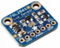
• Adafruit TSL2561 Digital Luminosity/Lux/Light Sensor Breakout

An advanced digital light sensor containing infrared and full spectrum diodes that detects light ranges from 0.1 to 40,000+ Lux.

Figure 5: Depicts Adafruit TSL2561 Digital Luminosity/Lux/Light Sensor Breakout

• SparkFun Sound Detector

An audio sensing board that is used to detect the amplitude of sound.

Figure 6: Depicts SparkFun Sound Detector

• ARDUINO MKR WIFI 1010

An open-source electronics platform used to read, manage and output electrical cur-rents from our sensors. It is also programmable through the Arduino programming language.

(21)

4.1.2 Software • Scikit-learn

Scikit-learn is a machine learning library for the python programming language. It features various tools for implementing classification, regression and clustering methods. Scikit-learn is designed to interoperate with other Python libraries such as NumPy, SciPy and Matplotlib. Scikit-learn is focused on Machine Learning. It is not concerned with the loading, handling, manipulating, and visualising of data. • Jupyter notebook

All the python scripts was programmed in Jupyter Notebook. Jupyter Notebook is a cell based web application editor that allows users to create and share documents that contain live code, equations, visualizations and narrative text. The Notebook has support for over 40 programming languages, including Python, R, Julia, and Scala. Notebooks can be shared with others using email, Dropbox, GitHub and the Jupyter Notebook Viewer. Code can produce rich, interactive output: HTML, images, videos, LaTeX, and custom MIME types.

• Arduino web editor

The arduino web editor is an online programming editor that is able to control the arduino hardware with code in the C, and C++, language. A downloadable integrated development environment (IDE) is also available but the web editor was chosen for this project because of its easy of use.

4.1.3 Experiment area

The experiment area is a study room located in the University of Malmös library in the Orkanen building, room code OR:B533. The room contains a number of chairs, one table as well as one television attached to the wall. The diameters of the room are as such; width 2 m, length 3.5 m, height 3 m. A visual representation can be found in Figure 1 and a plan of the room can be found in Figure 8.

(22)

4.2 Experiment description

A sensory prototype was put together using an Arduino, a sound detector, a light sensor, an air quality sensor and a PIR sensor. The air quality sensor has the ability to sense both CO2 ppm and TVOC ppm. The prototype was then programmed through the Arduino programming language, using the Arduino web editor.

The time interval to retrieve the sensor values was set to one second. The sensor values was then printed to the arduino "Serial Monitor" which uses a serial port on the computer to output the sensor values. To save the values from the sensors to a text file, a "port sniffer" was programmed through a python script to retrieve the values from the serial port, the values was then saved to a text file. A timestamp and a label that describes the occupancy count was also appended to the text file. Each line in the text file represents a data point.

Each data point is structured as follows:

timestamp|label|soundValue,lightValue,CO2Value,TVOCValue,PIRValue Below is an example of a line from the actual text file:

2019-04-10 12:27:22.381307|5|70,217.00,1017,93,1

Figure 9: Depicts arduino with sensors attached to study room wall

The prototype was then attached to the left of the door in the study room, at a height of 1.5 meters, as seen on Figure 9. A USB cable was then attached to the arduino and dragged outside of the room so that tests could be run without interference from the observers. The room was available for students to use throughout the day. Each student was informed that there was an experiment going on and that air quality, movement, light and sound would be measured. They were not informed how it was being measured or how they could impact the sensory data. Sensory data was collected once every second at two separate days as can be seen in Table 2.

Date Tuples created 2019-04-10 12745

2019-04-12 10195 Total 22940

(23)

Since there was no automatic way to determine occupancy count, the label that repre-sents occupancy count had to be manually changed each time the occupancy count changed. This meant that the entire system had to be restarted each time that the occupancy count changed. To restart the system takes about five to ten second so there was only a minor loss in data when the labels had to be changed. When all of the data had been collected it also had to be refactored since there was a bug in the "port sniffer" script that printed a new data point before the previous data point had printed all of the values. The bug happened on average once every forty-fifth second which amounts to a loss of about 4 minutes worth of data in a six hour period.

The content of the two text files collected on different days was then combined into one and that text file was then separated into three different text files, one for the timestamps, one for the labels and one for the sensory values. The collected data was then used to train six different machine learning algorithms through a python script that was written for this thesis. The following is pseudo-code of the script:

Algorithm 1 Pseudo-code of the script

1: v ← loadT ext(values.txt)

2: l ← loadT ext(labels.txt)

3: ts ← loadT ext(timestamps.txt)

4: ta ← length(values) ∗ 0.1 . The test amount

5: data ← getCombinationData(values) . Gets every combination of values

6: c ← getClassif iers() . Gets all six classifiers

7: mode ← [0All0,00 − 10]

8:

9: for each mode i do

10: if mode[i] equals ’0-1’ then

11: l ← reduceLabels() . Sets all labels >1 to 1

12: for each c j do

13: for each data k do

14: accuracyCounter ← 0

15: for five iterations do

16: results, model ← runClassif ier(c[j], data[k], l, ts, ta)

17: printT oF ile(results, model)

18: accuracyCounter+ = results.accuracy

19: printAverageAccuracy(accuracyCounter/5, c[j], data[k], mode[i])

The script works as follows:

1-3 The first three lines loads all of the data points into the script. The first line loads the sensory values from a text file, the second line loads the labels and the third line loads the timestamps.

4 The fourth line defines how the data points will be divided into training and testing samples. The testing amount is initialized to 10% of the data points so that 90% can be used for training.

(24)

5 The fifth line defines and initializes a variable ’data’ that is designed to hold every unique combination of sensory values (2N − 1). It contains every sensory value by itself, every unique combination of two sensory values, every unique combination of three sensory values, every unique combination of four sensory values and all values combined. With five sensory values, this calculates to 31 combinations ((2N − 1) = (25− 1) = 31).

6 The sixth line defines a variable which is initiated to store all six machine learning algorithms.

7 The seventh line defines a variable which is initiated to contain two string elements, ’All’ and ’0-1’. This variable is used to train the classifier model in two modes. The ’All’ mode trains the model to predict if the room is occupied by 0, 1, 2, 4 or 5 humans. The ’0-1’ mode trains the model to simply predict if the room is occupied or not by setting every label > 1 to 1.

9-15 Lines 9 through 15 is a series of loops designed to iterate through every possible unique combination of sensory values, machine learning algorithms and modes (’All’ and ’0-1’). That calculates to 372 iterations, ((25− 1)*6*2). For every one of those combinations, five classifiers where trained and evaluated. This was done to be able to calculate the average accuracy of five classifiers instead of just relying on the accuracy of a single classifier. The total number of trained and evaluated classifiers therefore calculates to 1860, ((25_{− 1)*6*2).}

16-18 Lines 16 through 18 is the part where the classifiers are actually trained and eval-uated. The code on line 16 is a call to the method ’runClassifier()’ that trains and evaluates the current iteration of classifier on the current iteration of data. The la-bels, timestamps and test amount is also passed as arguments to the ’runClassifier()’ method but those variables are not affected on the current iteration of the loops. In-side the ’runClassifier()’ method, the data is shuffled randomly. The data is shuffled partly so that the five classifiers that are trained on the same data is not identical, and partly to minimize the affect of training the classifiers on structured data that cluster similar data together. Line 17 prints the results to a text file and saves the trained model to a file. The results contains the accuracy of the classifier and just short of 2300 lines of predictions on the testing data.

19 Line 19 prints the average accuracy for each of the 372 unique classifiers to a text file. Each line in the text file contains the machine learning algorithm that was used, the sensor combination that was used, the mode that was used and the average accuracy. Following is a line from that text file:

KNeighbors Classifier,Light + TVOC,All,96.30340017436791

The script took about 40 minutes to complete on a laptop and resulted in 1860 text files with results, 1860 files of the saved models and one file with the average accuracy. The combined size of all the files is 915MB, which can be reduced to 148,4MB when compressed into a .zip file. The results were then analysed through Microsoft Excel.

(25)

5 Results

This section depicts the results in tabular form. For each table, a brief explanation of what the table represents can be found below the table. As can be seen in Table 3 a 100 percent accuracy was achieved when only classifying room occupancy detection, i.e. if the room was occupied or not. Whilst Table 4 shows a more varied result whereby K nearest neighbours showed the localised best result of 96,85% when light and CO2 sensors were used. Decision Tree Classifier showed 97,05% when using all sensors but PIR, Linear Discriminant Analysis showed 89,66% accuracy when using all sensors. Naive Bayes showed 92,37% using all sensors but TVOC, Random Forest Classifier showed an accuracy of 96,99% when using either Light, CO2 and PIR or Light, CO2 and TVOC, lastly Support Vector Machine had a accuracy of 96,63% when using all sensors but PIR.

Combination KN DTC LDA NB RFC SVM

CO2 + PIR 87,4% 89,4% 85,8% 66,8% 89,7% 88,9% CO2 + TVOC 86,2% 89,4% 85,5% 62,3% 89,1% 89,1% CO2 TVOC PIR 87,4% 89,7% 85,6% 62,7% 89,8% 89,2% Default 100,0% 100,0% 99,8% 95,7% 100,0% 100,0% Default minus CO2 100,0% 100,0% 99,8% 99,9% 100,0% 100,0% Default minus light 89,3% 88,5% 85,3% 62,2% 89,8% 89,1% Default minus PIR 100,0% 100,0% 99,8% 95,3% 100,0% 100,0% Default minus sound 100,0% 100,0% 100,0% 97,3% 100,0% 100,0% Default minus TVOC 100,0% 100,0% 99,8% 99,9% 100,0% 100,0% Light + CO2 100,0% 100,0% 100,0% 100,0% 100,0% 100,0% Light + PIR 100,0% 100,0% 100,0% 99,7% 100,0% 100,0% Light + TVOC 100,0% 100,0% 100,0% 100,0% 100,0% 100,0% Light CO2 PIR 100,0% 100,0% 100,0% 99,9% 100,0% 100,0% Light CO2 TVOC 100,0% 100,0% 100,0% 95,4% 100,0% 100,0% Light TVOC PIR 100,0% 100,0% 100,0% 100,0% 100,0% 100,0%

Only CO2 87,0% 89,5% 85,1% 66,9% 90,2% 89,2% Only light 100,0% 100,0% 100,0% 99,4% 100,0% 100,0% Only PIR 87,3% 89,0% 86,0% 63,8% 89,6% 86,1% Only sound 83,6% 85,5% 86,3% 85,9% 85,7% 86,0% Only TVOC 86,9% 89,0% 85,0% 62,9% 89,6% 86,4% Sound + CO2 89,3% 89,5% 85,6% 70,5% 89,8% 89,3% Sound + Light 100,0% 100,0% 99,8% 99,8% 100,0% 100,0% Sound + PIR 81,4% 86,0% 85,5% 85,9% 85,9% 85,6% Sound + TVOC 88,4% 90,4% 85,5% 66,0% 90,3% 87,2% Sound CO2 PIR 89,5% 88,5% 85,3% 70,7% 89,3% 89,6% Sound CO2 TVOC 88,6% 89,4% 85,8% 62,2% 89,9% 89,9% Sound Light CO2 100,0% 100,0% 99,8% 99,9% 100,0% 100,0% Sound Light PIR 100,0% 100,0% 99,8% 99,8% 100,0% 100,0% Sound Light TVOC 100,0% 100,0% 99,9% 99,9% 100,0% 100,0% Sound TVOC PIR 89,1% 90,3% 86,1% 66,4% 90,7% 87,0% TVOC + PIR 87,0% 89,6% 85,6% 63,9% 89,4% 85,4% Total Average 93,8% 94,6% 93,0% 83,9% 94,8% 94,1%

Table 3: This table shows the average accuracy of every combination when predicting room occupancy detection, i.e. if the room is occupied or not. Default means every sensor.

(26)

Combination KN DTC LDA NB RFC SVM CO2 + PIR 67,93% 72,93% 37,68% 58,00% 73,45% 71,11% CO2 + TVOC 67,78% 73,16% 50,06% 60,70% 73,12% 71,62% CO2 TVOC PIR 67,87% 73,40% 50,47% 61,27% 74,27% 71,00% Default 96,76% 96,67% 89,66% 81,28% 96,79% 96,22% Default minus CO2 96,22% 96,09% 81,48% 90,98% 96,01% 94,67% Default minus light 78,27% 77,70% 56,97% 61,02% 78,55% 78,95% Default minus PIR 96,63% 97,05% 89,49% 81,38% 96,71% 96,63% Default minus sound 96,52% 96,93% 87,78% 78,68% 96,68% 95,66% Default minus TVOC 96,76% 96,36% 81,47% 92,37% 96,34% 96,36% Light + CO2 96,85% 96,96% 77,18% 91,97% 96,84% 95,96% Light + PIR 78,18% 81,20% 81,47% 78,50% 81,33% 81,22% Light + TVOC 96,30% 96,63% 80,37% 91,62% 96,46% 94,66% Light CO2 PIR 96,80% 96,77% 76,26% 91,80% 96,99% 95,88% Light CO2 TVOC 96,71% 96,90% 87,68% 77,48% 96,99% 95,55% Light TVOC PIR 95,91% 96,50% 81,29% 91,51% 96,95% 93,99% Only CO2 66,22% 73,79% 36,97% 57,93% 72,66% 71,54% Only light 75,82% 80,99% 81,18% 79,97% 81,12% 82,07% Only PIR 65,58% 72,10% 43,03% 61,45% 72,68% 67,39% Only sound 44,17% 55,82% 49,52% 49,15% 56,36% 54,59% Only TVOC 64,87% 72,62% 43,67% 60,51% 72,65% 66,84% Sound + CO2 76,98% 78,00% 44,46% 62,28% 78,94% 79,43% Sound + Light 78,96% 82,67% 80,97% 72,50% 82,34% 81,18% Sound + PIR 47,15% 56,42% 49,87% 49,63% 56,63% 54,80% Sound + TVOC 76,44% 79,54% 49,75% 63,23% 80,18% 77,25% Sound CO2 PIR 77,85% 77,15% 44,13% 63,16% 77,88% 79,24% Sound CO2 TVOC 77,19% 78,47% 57,02% 61,26% 79,15% 78,83% Sound Light CO2 96,73% 96,54% 81,57% 92,07% 96,45% 96,18% Sound Light PIR 80,35% 82,76% 81,02% 72,91% 82,68% 81,70% Sound Light TVOC 96,45% 96,37% 81,19% 90,92% 96,22% 94,79% Sound TVOC PIR 75,93% 79,56% 47,78% 63,21% 79,25% 77,18% TVOC + PIR 66,68% 71,91% 43,29% 60,31% 72,14% 67,13% Total Average 80,4% 83,2% 65,3% 72,5% 83,4% 81,9%

Table 4: This table shows the average accuracy of every combination of machine learning algorithms and sensors when predicting room occupancy count, i.e. if the room had 0, 1, 2, 4 or 5 occupants. The green filling represents the best accuracy for every machine learning algorithm.

(27)

5.1 K Nearest Neighbours Classifier, Light + CO2.

The following depicts the best performing sensory values (Light + CO2) for this machine learning algorithm when predicting human occupancy count. Table 5 depicts the confusion matrix. Table 6 shows precision, recall and F-measure whilst Table 7 presents the overall results of the predictions. A weighted average with a precision of 0.97, Recall of 0.97 and F-measure of 0.97 was found. Out of 11470 tested tuples, 11109 was guessed correctly whilst 361 was incorrectly guessed.

predicted Correct 0 1 2 4 5 0 1639 1 3787 100 2 48 3901 2 34 4 5 370 73 5 41 58 1412 predicted Correct 0 1 2 4 5 0 100% 0% 0% 0% 0% 1 0% 97% 3% 0% 0% 2 0% 1% 98% 0% 1% 4 0% 0% 1% 83% 16% 5 0% 0% 3% 4% 93%

Table 5: K Nearest Neighbours prediction results and percentages.

Precision Recall F-measure Class

1,00 1,00 1,00 0 0,99 0,97 0,98 1 0,96 0,98 0,97 2 0,86 0,83 0,84 4 0,93 0,93 0,93 5 0,97 0,97 0,97 Weighted Avr.

Table 6: Precision, recall, F-measure for K Nearest Neighbours Classifier

Correctly classified 11109 0,968527 Incorrectly classified 361 0,031473

(28)

5.2 Decision Tree Classifier, Default minus PIR

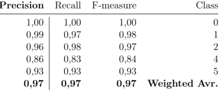
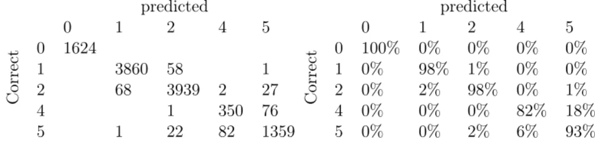
The following depicts the best performing sensory values (Default minus PIR) for this machine learning algorithm when predicting human occupancy count. Table 8 depicts the confusion matrix. Table 9 shows precision, recall and F-measure whilst Table 10 presents the overall results of the predictions. A weighted average with a precision of 0.97, Recall of 0.97 and F-measure of 0.97 was found. Out of 11470 tested tuples, 111132 was guessed correctly whilst 338 was incorrectly guessed.

predicted Correct 0 1 2 4 5 0 1624 1 3860 58 1 2 68 3939 2 27 4 1 350 76 5 1 22 82 1359 predicted Correct 0 1 2 4 5 0 100% 0% 0% 0% 0% 1 0% 98% 1% 0% 0% 2 0% 2% 98% 0% 1% 4 0% 0% 0% 82% 18% 5 0% 0% 2% 6% 93%

Table 8: Decision Tree Classifier prediction result

1,00 1,00 1,00 0 0,98 0,98 0,98 1 0,98 0,98 0,98 2 0,81 0,82 0,81 4 0,93 0,93 0,93 5 0,97 0,97 0,97 Weighted avr

Table 9: Precision, recall, F-measure for Decision Tree Classifier

(29)

5.3 Linear Discriminant Analysis, Default

The following depicts the best performing sensory values (Default) for this machine learning algorithm when predicting human occupancy count. Table 11 depicts the confusion matrix. Table 12 shows precision, recall and F-measure whilst Table 13 presents the overall results of the predictions. A weighted average with a precision of 0.90, Recall of 0.90 and F-measure of 0.89 was found. Out of 11470 tested tuples, 10284 was guessed correctly whilst 1186 was incorrectly guessed.

predicted Correct 0 1 2 4 5 0 1638 1 3648 173 2 3660 66 350 4 1 69 362 5 175 59 1269 predicted Correct 0 1 2 4 5 0 100% 0% 0% 0% 0% 1 0% 95% 5% 0% 0% 2 0% 0% 90% 2% 9% 4 0% 0% 0% 16% 84% 5 0% 0% 12% 4% 84%

Table 11: Linear Discriminant Analysis prediction result

1,00 1,00 1,00 0 1,00 0,95 0,98 1 0,91 0,90 0,91 2 0,36 0,16 0,22 4 0,64 0,84 0,73 5 0,90 0,90 0,89 Weighted avr

Table 12: Precision, recall, F-measure for Linear Discriminant Analysis

(30)

5.4 Naive Bayes, Default minus TVOC

The following depicts the best performing sensory values (Default minus TVOC) for this machine learning algorithm when predicting human occupancy count. Table 14 depicts the confusion matrix. Table 15 shows precision, recall and F-measure whilst Table 16 presents the overall results of the predictions. A weighted average with a precision of 0.93, Recall of 0.92 and F-measure of 0.92 was found. Out of 11470 tested tuples, 10595 was guessed correctly whilst 875 was incorrectly guessed.

Table 14: Naive Bayers prediction results

1,00 0,98 0,99 0 0,98 0,97 0,97 1 0,91 0,99 0,95 2 0,49 0,80 0,61 4 0,93 0,62 0,74 5 0,93 0,92 0,92 Weighted avr

Table 15: Precision, recall, F-measure for Naive Bayes

(31)

5.5 Random Forest Classifier, Light CO2 TVOC

The following depicts the best performing sensory values (Light CO2 TVOC) for this machine learning algorithm when predicting human occupancy count. Table 17 depicts the confusion matrix. Table 18 shows precision, recall and F-measure whilst Table 19 presents the overall results of the predictions. A weighted average with a precision of 0.93, Recall of 0.92 and F-measure of 0.92 was found. Out of 11470 tested tuples, 11125 was guessed correctly whilst 345 was incorrectly guessed.

predicted Correct 0 1 2 4 5 1 1644 2 3744 81 4 35 4004 27 5 3 338 93 predicted Correct 0 1 2 4 5 0 100% 0% 0% 0% 0% 1 0% 98% 2% 0% 0% 2 0% 1% 98% 0% 1% 4 0% 0% 1% 78% 21% 5 0% 0% 3% 4% 93%

Table 17: Random Forest Classifier prediction results

1,00 1,00 1,00 0 0,99 0,98 0,98 1 0,97 0,98 0,98 2 0,84 0,78 0,81 4 0,92 0,93 0,93 5 0,97 0,97 0,97 Weighted avr

Table 18: Precision, recall, F-measure for Random Forest Classifier

(32)

5.6 Support vector machine, Default minus PIR

The following depicts the best performing sensory values (Default minus PIR) for this machine learning algorithm when predicting human occupancy count. Table 20 depicts the confusion matrix. Table 21 shows precision, recall and F-measure whilst Table 22 presents the overall results of the predictions. A weighted average with a precision of 0.93, Recall of 0.92 and F-measure of 0.92 was found. Out of 11470 tested tuples, 11083 was guessed correctly whilst 387 was incorrectly guessed.

Table 20: Support Vector Machine prediction results

1,00 1,00 1,00 0 1,00 0,97 0,98 1 0,96 0,99 0,97 2 0,77 0,80 0,79 4 0,93 0,91 0,92 5 0,97 0,97 0,97 Weighted avr

Table 21: Precision, recall, F-measure for Support Vector Machine

(33)

5.7 Collective machine learning results

A comparison between all the best combinations for each machine learning algorithm can be found in Table 23.

K Nearest Neighbours Classifier Light + CO2 Correctly classified 96,85% Incorrectly classified 3,15%

Precision 0,97

Recall 0,97

F-measure 0,97

Decision Tree Classifier Default minus PIR Correctly classified 97,05%

Incorrectly classified 2,95%

Precision 0,97

Recall 0,97

F-measure 0,97

Linear Discriminant Analysis Default Correctly classified 89,66% Incorrectly classified 10,34%

Precision 0,90

Recall 0,90

F-measure 0,89

Naive Bayes Default minus TVOC

Correctly classified 92,37% Incorrectly classified 7,63%

Precision 0,93

Recall 0,92

F-measure 0,92

Random Forest Classifier Light CO2 TVOC Correctly classified 96,99%

Precision 0,97

Recall 0,97

F-measure 0,97

Support Vector Machine Default minus PIR Correctly classified 96,63%

Precision 0,97

Recall 0,97

F-measure 0,97

(34)

6 Discussion

6.1 Method discussion

This section will discuss the different methods described in section 4. This section will discuss the choice of hardware, software and location as well as the method for retrieving data and its processing and analysis.

6.1.1 Material

The hardware was provided by the Internet of Things and People (IoTaP) Research Center of Malmö university and was made to be used in another experiment by the department. After some issues with the setup, such as the arduino mkr having too little power to run an additional ultrasound sensor, a choice was made to only use the four sensors mentioned in section 4. Due to some early issues in making the prototype we were provided with the sensors and arduino fairly late into the course and as time was limited some issues started to arise when the experiments began. One such issue was that an optimal placement of the PIR sensor could not be found and it therefor provided us with false positives when registering movement in the room, when it was not occupied, it was further never found why it did this.

The choice of room was also provided by the IoTaP center, as the prototype was designed to be placed in three study rooms in the university library, two small identical rooms and one larger conference room. Prior tests were run in both rooms, but since there was an issue with the first version of the port sniffer script, the data was lost. After looking at the data of both the large room and the small room as well as keeping the time limitation in mind we chose to only run the next tests in the smaller room.

The observation method chosen was observer as participant. This choice was made since we concluded that it was an opportune moment to run an experiment where the room was not occupied by us or anyone with any knowledge in how the experiment was run. It was instead used by students whom themselves chose to use the room that day. An additional reason to why we chose this observation method was since as far as we could conclude it had not been done before.

When it came to the choice of what programming language to be used, we chose the python language for running the port sniffer as well as the machine learning algorithms. This choice was made by suggestion of our supervisor since we did not have any prior experience in the language and found it to be a perfect opportunity to learn a new lan-guage. The choice of language did also provide us with a number of libraries for already made MLMs from which we chose our six different machine learning methods. The choice of MLMs was furthermore based on what was regularly found to be used in articles on occupancy detection from our research in section 3.

6.1.2 Data retrieval

Due to the time limitations there was a number of issues that arose with the data when running the experiment. The first version of the port sniffer was made to put timestamps, labels and sensory data in three separate files. Due to us needing to check that the data was printed as designed we opened the files at a number of points which we found later

(35)

made the script unable to write to that file during the timeframe of which it was opened. This made the three files out of sync and unusable. Also since there was no automatic detection of how many were occupying the room at a certain time the tests had to be run manually with an observer sitting outside of the room and restarting the script each time the occupancy number changed. This put us in a challenging situation since we had to physically be there. Our prefered design was to have an automatic occupancy detection system so that we could retrieve data continuously over multiple days. But due to limited time and hardware this could not be achieved and only two days of data could be retrieved. This also ended up with us choosing to retrieve data every second since there was only a limited timeframe in which the experiment could be run and we needed a large amount of data for the MLMs.

Due to choosing a non fully participating observational method we also found that the tests subjects all chose to turn off the lights when leaving the room empty. This most probably had an affect on the results of the experiments since it was found that lighting had a large effect on the machine learning methods.

6.1.3 Training and analysis

When creating the training setup for the MLMs we found that there was a need to test the MLMs multiple times to achieve an acceptable average for each MLM and thereby validate the tests. We looked at a multitude of validation methods such as the k fold cross validation method. But we chose to only randomise the data and train it on 90% of the data and test it on 10% since there was not much of a difference in result found between the different validation methods.

The choice of using Microsoft Excel to analyse the data was made since the team had a lot of prior knowledge in data management in Excel. This created an issue when analysing the different combinations of sensors and MLMs, since the method of creating the different tables and confusion matrices could not be automated. This concluded in a number of time consuming data processing steps had to be made before each confusion matrix was to be created. This evolved into us making the decision to only run the confusion matrix test on the best combinations of sensors and MLMs.

When analysing the data we found that there was a risk of the MLMs making a wrong classification and it not showing in the data. To combat this risk we realised that the best method to use was a confusion matrix. By creating a confusion matrix for each combination of sensors and MLMs we could validate that the results from the experiment was actually correct.

6.2 Result discussion

This section is designed for discussing the results showed in section 5. This section will discuss how the results answers the three research questions found in section 1.2. This section will also discuss and compare the results of similar projects and why their results might, or might not, be similar to the results of this thesis.

(36)

6.2.1 Answering the research questions.

Following is the three research questions found in section 1.2 and a discussion on how the results showed in section 5 answers them.

1. What combination of sensors and machine learning algorithms gives the best accuracy for classifying human occupancy in a university study room? Lets start by looking at Table 3. Table 3 depicts the results of training classifiers to predict room occupancy detection, i.e. if the room is occupied or not. All of the machine learning algorithms managed to achieve an accuracy of 100% on multiple combination of sensors and every single sensor is represented in a combination where the accuracy is 100%. Since multiple combinations has achieved an accuracy of 100%, the question cannot be answered decisively without looking more in depth.

By looking at the last row in Table 3, a row called ’Total Average’ can be found. This row represents the total average of every accuracy that a certain machine learn-ing algorithm managed to achieve. The total average for most machine learnlearn-ing algorithms is in a very tight cluster, within 1% of each other, the exception being NB (Naive Bayes) which scored >10% lower than the rest. RFC (Random Forest Classifier) achieved the highest total average with 94,8%, which is 0.2% higher than the second highest DTC (Decision Tree Classifier) and 0.7% higher than the third highest SVM (Support Vector Machine). While the total average does not answer the question directly, an argument can be made that RFC outperformed the other machine learning algorithms, if only just barely.

By looking at the results for when every lone sensor was used, i.e. ’Only CO2’, ’Only light’, it becomes clear that the light sensor outperformed the rest of the sensors in terms of accuracy. The light sensor was the only lone sensor that managed to achieve an accuracy of 100% with all machine learning algorithms except NB, which achieved a 99,4% accuracy. It is important to note that the high accuracy of the light sensor is most likely correlated to the fact that during the data-gathering phase, the last occupant leaving the room always shut the lights off and the first occupant entering the room always turned the light on. This means that the collected data has little to no examples of an unoccupied room with the lights on and little to no examples of an occupied room with the lights off. This is most likely also why every combination that achieved a 100% accuracy involved the light sensor.

While a direct and decisive answer to the question cannot be made, an argument could be made that the RFC algorithm in combination with the light sensor gives the best accuracy for determining room occupancy detection. These results are similar to Luis et al [26]. which worked on occupancy detection with multiple sensors and multiple machine learning algorithms and reported that the light sensor achieved the highest accuracy, between 97% and 99%. Their work also reported that a version of the DT algorithm called "CART" achieved the highest accuracy while in this work the DT algorithm came in as a close second behind the RTC algorithm.

Lets shift the attention to Table 4, which depicts the results of training classifiers to predict occupancy count. In this table, no combination managed to achieve an accuracy of 100%. In terms of the ’Total Average’ row, the highest total average in

(37)

Table 4 is lower than the lowest total average in Table 3. This is to be expected as multi-class classification is often more difficult than binary classification. RFC achieved the highest total average accuracy at 83,4%, which is again 0,2% higher than DTC. It is DTC, however, that achieved the highest accuracy with a single combination at 97,05%, this was achieved with the combination ’Default minus PIR’. RFC achieved the second highest accuracy with a single combination at 96,99%, this was achieved with both ’Light CO2 PIR’ and ’Light CO2 TVOC’. In this table, the lone sensor that achieved the highest accuracy was also the light sensor. The fact that the light sensor achieved the highest accuracy in Table 3 is not surprising since the light was always off when the room had no occupants and the light was always on when the room had occupants. This has little affect when predicting occupancy count however and it is interesting that the light sensor convincingly outperformed the other sensors. These results are however not consistent with results of Irvan et al [2]. results which reported that illumination level is not highly correlated to number of occupant, or with Ebenezer et al [23]. results which reported that light features performed the worst. These differences in results could be correlated to a difference in environment. The articles just mentioned had an environment that was larger than the environment used in this thesis, they also had windows which could affect the light sensor readings. The results of this thesis are also not consistent with Amayri et al [28]. results which reported that acoustic pressure was identified as one of the most important feature for occupancy classification. The results of this thesis found that the sound sensor was the worst sensor for both occupancy detection and occupancy count.

2. What is the minimal combination of sensors and machine learning algo-rithms needed for 90 percent accuracy in human occupancy recognition? Lets again break this question down by room occupancy detection and room occu-pancy count. In Table 3, occuoccu-pancy detection, there are many combinations that achieved an accuracy above 90% but the minimal combination is with a lone light sensor and any machine learning algorithm. This result might be misleading however and it might not apply to situations where occupants leave the light on when they leave or when occupants prefer to work with the lights off. There is however another combination that achieved an accuracy of 90,2%, which is with the use of the CO2 sensor and the RFC algorithm. This combination has no apparent misleading factors and could be generalized to hold true in other similar situations. There exists other combinations which achieved an accuracy >90% although these combinations used more than one sensor.

In Table 4, occupancy count, there are also many combinations that achieved an accuracy >90%. Though no lone sensor was able to achieve an accuracy >90%, there exist some combinations that achieved it. All combinations that achieved an accuracy >90% was in a combination that included the light sensor. No combination without the light sensor achieved an accuracy >90%. The most minimal combination that achieved an accuracy >90% was the ’Light + CO2’ sensor combination with the DTC algorithm with an accuracy of 96,96%.

(38)

3. What single sensor, if any, outperformed the rest, and what single machine learning algorithm outperformed the rest in classifying human occupancy in a room?

In terms of the question ’What single sensor outperformed the rest?’, the answer in both Table 3, occupancy detection, and Table 4, occupancy count, is clearly the light sensor. While the light sensor results in Table 3 might be misleading, the light sensor results in Table 4 is almost certainly not misleading.

The question ’What single machine learning algorithm outperformed the rest?’ is a little harder to answer since it depends on a lot of factors. However, the two machine learning algorithms that consistently achieved high a high accuracy, both in occupancy detection and occupancy count, is the RFC algorithm and the DTC algorithm. The RFC algorithm outperformed all other algorithms in the total average accuracy, both in occupancy detection and occupancy count. The DTC algorithm was a close second to RFC in total average accuracy but achieved the highest accuracy for a combination in Table 4 occupancy count. An argument can be made for both the RFC algorithm and the DTC algorithm as the best machine learning algorithm for this situation.

7 Conclusion and future work

The focus of this thesis was to determine an optimal approach to human occupancy recog-nition, i.e. if there exists a certain combination of sensors and machine learning algorithm that outperformed the rest. By analyzing the results of this thesis it is clear that there exists such a combination. The results, however, are most likely bound to the particular methods and environment used in this thesis. By reading the results of similar projects and by analyzing the results in this thesis it is safe to say that human occupancy recognition is highly situational and that the findings from one project can often not be extrapolated to be effective in other situations. An argument could be made that with a situation that is very similar to the one found in this thesis, a light sensor will do well in occupancy detection and a light sensor in combination with a CO2 sensor will do well in occupancy count.

The data-gathering phase of this thesis experienced some difficulties and as a result, several days worth of data had to be thrown away as the process was improved. This was especially frustrating since the data-gathering phase required a person to manually oversee the entire data-gathering phase. The original plan was to have an automated data-gathering system. This system would have sensors installed in three different rooms and would send the information to a database. The automated system would also include a special camera that could detect the occupancy count. This system would be a huge improvement to the current data-gathering system implemented in this thesis. It would reduce or eliminate corrupt data and would also eliminate the need to manually oversee the entire data-gathering phase. Future work would therefore include a similar data-gathering system. The plan was also to gather data from the three different rooms. The data collected from the different rooms would be used both separately and combined to train a classifier and the results would be compared. These results would give an indication if it is possible to build a more general classifier that is capable of detecting human occupancy

(39)

in a variety of environments. Since this was not done in this thesis it would be included in future works.

(40)

References

[1] A. K. R. B. A. S. A. E. C. M. D. S. S. N. Varick L. Erickson, Yiqing Lin, “Energy efficient building environment control strategies using real-time occupancy measure-ments,” Proceedings of the First ACM Workshop on Embedded Sensing Systems for Energy-Efficiency in Buildings - BuildSys ’09, p. 19, 2009.

[2] F. D. S. M. H. Irvan Bastian, Arief Ang, “Human occupancy recognition with multi-variate ambient sensors,” 2016 IEEE International Conference on Pervasive Comput-ing and Communication Workshops (PerCom Workshops), pp. 1–6, 2016.

[3] L. M. Candanedo and V. Feldheim, “Accurate occupancy detection of an office room from light, temperature, humidity and co2 measurements using statistical learning models,” Energy and Buildings, vol. 112, pp. 28–39, 2016.

[4] R. H. Dodier, G. P. Henze, D. K. Tiller, and X. Guo, “Building occupancy detection through sensor belief networks,” Energy and buildings, vol. 38, no. 9, pp. 1033–1043, 2006.

[5] R. Zhang, K. P. Lam, Y.-S. Chiou, and B. Dong, “Information-theoretic environment features selection for occupancy detection in open office spaces,” in Building Simula-tion, vol. 5, pp. 179–188, Springer, 2012.

[6] C. Tsai and M.-S. Young, “Pyroelectric infrared sensor-based thermometer for moni-toring indoor objects,” Review of scientific instruments, vol. 74, no. 12, pp. 5267–5273, 2003.

[7] “Technical overview of volatile organic compounds,” Apr, https://www.epa.gov/indoor-air-quality-iaq/technical-overview-volatile-organic-compounds 2017.

[8] A. Industries, “Adafruit tsl2591 high dynamic range digital light sensor, https://www.adafruit.com/product/198,” August 2018.

[9] S. Electronics, “Sparkfun sound detector, https://www.sparkfun.com/products/12642.”

[10] D. A. D. t. O. Sam McCandlish, Jared Kaplan, “An empirical model of large-batch training,” 2018.

[11] N. S. Altman, “An introduction to kernel and nearest-neighbor nonparametric regres-sion,” The American Statistician, vol. 46, no. 3, pp. 175–185, 1992.

[12] L. Breiman, J. H. Friedman, R. A. Olshen, and C. J. Stone, “Classification and re-gression trees. belmont, ca: Wadsworth,” International Group, p. 432, 1984.

[13] S. Balakrishnama and A. Ganapathiraju, “Linear discriminant analysis-a brief tuto-rial,” Institute for Signal and information Processing, vol. 18, pp. 1–8, 1998.

[14] P. Domingos and M. Pazzani, “On the optimality of the simple bayesian classifier under zero-one loss,” Machine learning, vol. 29, no. 2-3, pp. 103–130, 1997.