Sound localization for human interaction in real environment

(1)

Sound localization for human interaction in real environment

Ralf Strömberg

Stig-Åke Svensson

Mälardalen University School of Innovation, Design and Engineering

16/06/11

Supervisor

Lars Asplund, Mälardalen University

Patrik Björkman, Robyn Robotics AB

Examiner

Lars Asplund, Mälardalen University

(2)

Abstract

For a robot to succeed at speech recognition, it is advantageous to have a strong and clear signal to interpret. To facilitate this the robot can steer and aim for the sound source to get a clearer signal, to do this a sound source localization system is required. If the robot turns towards the speaker this also gives a more natural feeling when a human interacts with the robot. To determine where the sound source is positioned, an angle relative to the microphone pair is calculated using the

interaural time difference (ITD), which is the difference in time of arrival of the sound between the pair of microphones. To achieve good result the microphone signals needs to be preprocessed and there are also different algorithms for calculating the time difference which are investigated in this thesis. The results presented in this work are from tests, with an emphasis on focusing at real-time systems, involving noisy environment and response time. The results show the complexity of the balance between computational time and precision.

Abstrakt

För att en robot ska lyckas med taleigenkänning, är det fördelaktigt att ha en stark och tydlig signal att tolka. För att underlätta detta kan roboten styra och rikta in sig mot ljudkällan för att få en tydligare signal och för att detta skall vara möjligt krävs ett system för lokalisering av ljudkällan. Om roboten vänder sig mot talaren ger detta även en mer naturlig känsla när en människa

interagerar med roboten. För att avgöra var ljudkällan är placerad, beräknas en vinkel i förhållande till mikrofonparet med hjälp av interaurala tidsskillnaden (ITD), vilket är skillnaden i ankomsttid av ljudet mellan mikrofonparet. För att uppnå bra resultat måste mikrofonsignalerna förbehandlas och det finns också olika algoritmer för att beräkna tidsskillnaden som undersöks i detta examensarbete. Det resultat som presenteras i detta arbete kommer från tester, med tonvikt på att fokusera på realtidssystem, som inbegriper bullrig miljö och svarstid. Resultaten visar komplexiteten i balansen mellan beräknings tid och precision.

(3)

We would like to thank

Lars Asplund for good support and help

Mikael Ekström for providing equipment and help

Patrik Björkman and Lasse Odens Hedman for help with the demonstration

(4)

7.4.1 Using FFT-implementation...57 7.4.2 Using Algorithm 4...58 7.5 Discussion...59 8 Conclusions...61 8.1 Results...61 8.2 Discussion...62 8.3 Future work...62 9 References...64 Appendix A ...66 Appendix B ...67 Appendix C ...68 Appendix D ...70 Appendix E ...76 Appendix F ...80 Appendix G ...82 Appendix H ...84 Appendix I ...85 Appendix J ...93 Appendix K ...97

(6)

List of Images

Image 1.1: Azimuth ITD...2

Image 1.2: Sensitivity typical condenser microphone...7

Image 1.3: Polar pattern...8

Image 1.4: Non-inverting amplifier...9

Image 1.5: Filter Bode diagram...11

Image 1.6: RC filter...12

Image 1.7: Half of one LSB offset...13

Image 1.8: Basic integrator...14

Image 1.9: Trade-offs among different ADC ...15

Image 1.10: Periodic sine...16

Image 1.11: Discontinued sine...16

Image 1.12: Spectral leakage...16

Image 1.13: Window function...16

Image 1.14: Different windows in time-domain...17

Image 4.1: The testing area...24

Image 4.2: The microphone set up...25

Image 4.3: The protractor...25

Image 4.4: The sound source set up...26

Image 4.5: Microphone amplifier with filter...27

Image 4.6: Reset_Debounce component...29

Image 4.7: clkScaler component...29

Image 4.8: ADC_Deserializer component...30

Image 4.9: Dual_ADC_Controller component...30

Image 4.10: transmiter2 component...31

Image 4.11: Initially miscalculation...32

Image 4.12: The original sound source...33

Image 4.13: Dataset1, omnidirectional microphones over the full length of the signal...36

Image 4.14: Dataset1, Noise cancelling microphones over the full length of the signal...37

Image 4.15: Dataset1, Noise cancelling microphones windowed , window size: 0.01s...37

Image 4.16: Dataset1, Noise cancelling microphones windowed , window size: 0.01s...38

Image 4.17: Dataset1, omnidirectional microphones windowed , window size: 0.01s...38

Image 4.18: Dataset1, omnidirectional microphones windowed , window size: 0.01s...39

Image 4.19: Omnidirectional, sampling size 2000...39

Image 4.20: GCC on 70 degrees...40

Image 4.23: Noise-cancelling, sampling size 2000...41

Image 5.1: Speaker set up for testing with noise from the front ...45

Image 5.2: Speaker set up for testing with noise from the back...46

Image 5.3: Results when noise is generated from the front...47

Image 5.4: Results when noise is generated from behind...47

Image 5.5: Results(filtered) when noise is generated from the front...48

Image 5.6: Results(filtered) when noise is generated from behind...48

Image 5.7: Front Noise, omnidirectional microphones...48

Image 5.8: Front Noise, noise-cancelling microphones...48

Image 5.9: Back Noise, omnidirectional microphones...49

(7)

Image 5.10: Back Noise, noise-cancelling microphones...49

Image 6.1: Elevation test, omnidirectional microphones...52

Image 6.2: Elevation test, noise cancelling microphones...52

Image 6.3: Omnidirectional microphones with different elevation...52

Image 6.4: Noise-cancelling microphones with different elevation...53

Image 7.1: Example, 10 degrees from elevation 0.9...57

Image 7.2: Response-time, without noise...57

Image 7.3: Response-time, with noise...57

Image 7.4: Response time 0.256, omnidirectional mic with no noise...58

Image 7.5: Response time 0.256, noise-cancelling mic with no noise...58

Image 7.6: Response time 0.256, omnidirectional mic with front noise...59

Image 7.7: Response time 0.256, noise-cancelling mic with front noise...59

Image 8.1: Sound source localization with three microphones...63

(8)

List of Tables

Table 1.1: Key terms for different window functions...18

Table 4.1: FPGA in- & out-puts...28

Table 4.2: Reset_Debounce in- & out- ports...29

Table 4.3: clkScaler in- & out-ports...29

Table 4.4: ADC_Deserializer in- & out-ports...30

Table 4.5: Dual_ADC_Controller in- & out-ports...30

Table 4.6: transmiter2 in- & out-ports...31

Table E.1: Dataset1, Noise cancelling mic over the full length of the signal,Image 4.14...76

Table E.2: Dataset1, omnidirectional mic over the full length of the signal,Image 4.13...76

Table E.3: Dataset1, noise cancelling mic, window size 0.01s, Image 4.15 & Image 4.16...76

Table E.4: Dataset1, omnidirectional mic, window size 0.01s, Image 4.17 & Image 4.18...76

Table E.5: Data set 1, omnidirectional, time window 0,1 s, Image 4.19...77

Table E.8: Data set 1, noise-cancelling, time window 0,1 s, Image 4.23...78

Table F.1: Noise from the front results for FFT, Image 5.3...80

Table F.2: Noise from the back results for FFT, Image 5.4...80

Table F.3: Noise from the front results for filtered FFT, Image 5.5...80

Table F.4: Noise from the back results for filtered FFT, Image 5.6...80

Table F.5: Dataset 2, Front omnidirectional mic, Image 5.7...80

Table F.6: Dataset 2, Front noise-cancelling mic, Image 5.8...81

Table F.7: Dataset 2, Back omnidirectional mic, Image 5.9...81

Table F.8: Dataset 2, Back noise-cancelling mic, Image 5.10...81

Table G.1: Elevation results for FFT using omnidirectional microphones, Image 6.1...82

Table G.2: Elevation results for FFT using noise cancelling microphones, Image 6.2...82

Table G.3: Dataset 3, omnidirectional mic using median or mode function, Image 6.3 ...82

Table G.4: Dataset 3, noise-cancelling mic using median, similar to Image 6.4 ...82

Table G.5: Dataset 3, noise-cancelling mic using mode function, Image 6.4...83

Table H.1: Elevation 0.9, Image 7.2...84

Table H.2: Noise Front, 0.9, Image 7.3...84

Table H.3: Response time 0.256, omnidirectional mic with no noise, Image 7.4...84

Table H.4: Response time 0.256, noise-cancelling mic with no noise, Image 7.5...84

Table H.5: Response time 0.256, omnidirectional mic with front noise, Image 7.6...84

Table H.6: Response time 0.256, noise-cancelling mic with front noise, Image 7.7 ...84

(9)

Abbreviations

ADC - Analog-to-digital Converter CC - Cross-correlation

CS - Cross Spectrum

CORDIC - Coordinate Rotation Digital Computer DAC - Digital-to-analog Converter

DFT - Discrete Fourier Transform DNL - Differential Non-linearity ENOB - Effective Number Of Bits

FFT - Fast Fourier Transform

FPGA - Field-programmable Gate Array FT - Fourier Transform

GCC - Generalized Cross-correlation HRTF - Head Related Transfer Function

IFFT - Inverse Fast Fourier Transform ILD - Interaural Level Difference INL - Integral Non-linearity ITD - Interaural Time Difference LSB - Least Significant Bit

ME - Mean Energy

ML - Maximum Likelihood MSB - Most Significant Bit PHAT - Phase Transform

RMSE - Root Mean Square Error SAR - Successive Approximation

SHOSLIF - Self-organizing Hierarchical Optimal Subspace learning & Inference Framework SNR - Signal-to-noise Ratio

TDOA - Time Difference Of Arrival

VHDL - VHSIC Hardware Description Language VHSIC - Very High Speed Integrated Circuit

(10)

1 Introduction

Until the mid-1900s was the scientific theory that humans localize sounds with Interaural Level Difference (ILD). The idea is to measure the energy or level difference between a pair of ears, or microphones, to estimate the sound source localization. The method is still usable, but has several drawbacks and isn't very accurate. Instead, a new theory which is about Interaural Time Difference (ITD) and measuring the time difference when the sound wave reaches the microphone pair.

Todays applications that make use of sound localization system is for example underwater sonar which works with ITD, concert halls for measuring the acoustics, conference for aiming speaker microphone to amplitude the speaker and robots for steering towards the speaker, which improve speech recognition and social interaction.

This thesis's intention is to study and apply sound localization methods for a robot produced by Robyn Robotics [1].

1.1 Background

This section describes the necessary theory in order to facilitate further reading, such as the

mathematical theories to grant the reader a better understanding for the concepts that are presented in this thesis, such as Fourier Transformation.

1.1.1 Interaural time difference (ITD)

To be able to determine the azimuth one common way is to use a model, shown in Image 1.1, that gives a reasonable approximation of azimuth. Azimuth is the angular measurement in a spherical coordinate system. This model can be used for each pair of microphones used.

(11)

Where DA and DB is the distance between the sound source and microphone A and B respectively, b is the difference in the distances DA and DB and d the distance between microphone A and B . There is an inexactness of b and this is due to that in a reality the vectors DA and DB are not parallel but intersects at the sound source. The accuracy of the model will therefore decrease the closer the sound source is to the microphone pair. Using this model the azimuth is equal to the angle  and by using the definition of sine,  can be calculated in the following way.

≈arcsin



b

d



(1.1)

Since the distance d is known the problem then becomes an issue of determining the distance of

b . It is known that the distance b is an approximation of the difference in distance between D_A and DB . Using the time difference of arrival (TDOA) of a sound between microphone

A and B it is possible to calculate the distance travelled by multiplying the TDOA with the

speed of sound.

b≈ D_A−D_B≈V_Sound∗T (1.2)

Where  T is the TDOA and VSound is the speed of sound through the air. By combining equations 1.1 and 1.2 the resulting equation 1.3 is.

≈arcsin



VSound∗T

d



(1.3)

Where the only unknown variable is  T . There are a number of ways to calculate  T . The methods mostly used for doing this in artificial sound source localization will be discussed bellow.

1 Introduction 2

(12)

1.1.2 Complex Numbers

Complex numbers consists of a real and an imaginary part. This can easily be expressed in the rectangular form z=abi where z is the complex number, a and b are real numbers and

i is the standard imaginary unit which has the property i=



−1 . The two separate values mean that z can be seen as a set of coordinates where a is coordinate on the real-axis and

b is the coordinate on the imaginary-axis.

With this knowledge it is possible to represent z in an additional way, namely using polar coordinates. This gives us z =r



cos i∗sin 



where r=



a2b2 , from Pythagoras theorem, and is the distance ( magnitude) from origin and  is the angle from the real axis.

With the complex number z expressed in polar coordinates it is possible to use Euler´s Formula

ei _{=cos i∗sin  to express it as z=r∗e}i  _.

1.1.2.1 Complex conjugate

The complex conjugate of a complex number can be created by changing the sign of the imaginary part of a complex number. Thus, if z is the complex number:

z =abi (1.4)

then the complex conjugate of z is:

z =a−bi (1.5)

and for polar coordinates without using and with using Euler´s notation respectively:

z =r



cos−i∗sin 



(1.6)

z =r∗e−i  _(1.7)

1.1.3 Fourier Transform

The concept of the Fourier transform (FT) can be divided into two parts. Firstly, the act of transforming a signal from being dependant on time, in the time domain, to being dependant on frequency, the frequency domain. Secondly FT sometimes refers to the signal once it has been transferred to the frequency domain. For the convince of the reader FT will in this paper refer to the act of transformation while the the frequency dependant signal will be referred to as being in the frequency domain.

(13)

Let f t be a continuous signal of a real variable t , normally time. The continuous FT of

f t is then defined by the equation: F =

_∫

∞ −∞

f t e−i2  t_dt

(1.8)

Where F  is the signal in the frequency domain and  is the frequency coefficient. It should also be known that for each FT there is an inverse to the transformation:

f t=

_∫

∞ −∞

F ei2  t_{d }

(1.9)

This transformation transforms a signal in the frequency domain back into the time domain.

1.1.4 Discrete Fourier Transform

Since the FT only deals with continuous signals it is not applicable to signals that have been sampled and digitalized. For this the discrete Fourier transform (DFT) can be used instead.

G=

∑

n =0 N −1 g n e −2  i  n N _(1.10)

Where g  n is a sequence that consists of N complex numbers and transforms it into an equally long sequence G . The inverse of this transformation is defined as.

g  n= 1 N

∑

=0 N −1 G  e 2  i n N _(1.11)

These can be used to transform a discrete signal back and fourth between the time domain and the frequency domain.

1.1.5 Fast Fourier Transform

Fast Fourier Transform (FFT) isn't really a different transformation but rather refers to several different algorithms for calculating the DFT in a much faster way. Examples of these are the Cooley-Tukey algorithm, Danielson-Lanczos algorithm, Prime-factor FFT algorithm, Bruun's FFT algorithm, Rader's FFT algorithm and Bluestein's FFT algorithm [2].

1.1.6 Cross Spectrum

The Cross Spectrum(CS) of the signals g  n and h n is the the product of G and the complex conjugate H  of H  . Thus the CS, FGH , can be calculated by:

(14)

F_GH=G ∗H  (1.12)

1.1.7 Cross-correlation

A common solution for determine time difference of arrival for two signals is cross-correlation (CC), which is similar to convolution with the exception of not reversing the signal, before shifting it and multiplying by the other. CC works best for sound signals between 300 – 1500 Hz, due to that they are easier to sample with good resolution and the sound wavelength is long. Cross-correlation measuring the similarity of two waveform signals and can estimate the time delay between them and the discrete cross-correlation is defined as equation 1.13.

r_ij =

∑

n=0 N −1

x_i[n ] x_j[n−] (1.13)

N is number of samples, the signal received of microphone i is xi[n ] and  is the correlation lag, where r_ij is maximized when  is equivalent with the correct time difference of the two signals. Cross-correlation works good with whitening sound, but has a high complexity O N2_

and sensitive to noise and reverberations [3] and therefore not suitable for real environments. Generalized cross-correlation is a more robust method and less computer demanding and is based on transforming the signals from time domain to the frequency domain using Fourier transformation and then calculating the CS as shown in equation 1.14 below.

Rij=Xi[k ] X j[k ] (1.14)

The CS is equivalent to FT of r_ij _{and it is possible to transform back and fourth between the}

CS and CC using FT and IFT. Thus the inverse Fourier transform of equation 1.14 represent the cross-correlation as shown in equation 1.15.

r_ij = 1

N

∑

k =0 N −1

X_i[k ] X _j[k ]ei2 k / N (1.15)

For more improvements a weighting function can be defined as in equation 1.16. The weighting function can sharpen the peak of correlation, which leads to better accuracy. The most common weighting functions are maximum likelihood (ML), the phase transform (PHAT), which will be described later in the rapport and bandpass weighting function.

rij=_N1

∑

k =0 N −1 W k  Xi[k ] X j[k ]e i2  k / N (1.16) 1 Introduction 5

(15)

1.1.8 Phase Transform (PHAT)

Phase transform is a weighting function for cross-correlation as described earlier in this thesis and improve the robustness and precision in more realistic environment. PHAT is popular weighting function in others work [4] [5] [6] [7] [8] [9] [10] [11] [12] [13] [14] especially for real-time system, due to it's robustness in environments which may contain echoes and noise.

PHAT normalizes all values in the frequency spectrum, which means that the correlation is only calculated for the discrete phase angles of the signal, which reduce the effect of echo. Equation (1.17) below simply divides 1 by the absolute value of cross-spectrum, which normalizes the magnitude with multiplication by the cross-spectrum.

W_PHATk = 1

∣

X_ik  X_jk 

∣

(1.17)

Another approach to PHAT is the PHAT-β and PHAT-β weight the PHAT by varying the parameter β, giving the normalizing different effects. This can help the precision further by not calculating the cross-correlation depending only on the phase angles, but also give some smaller weight to the magnitude. The difficulty can be finding a effective value of β and other works [11] [13] has found that 0,65 and 0,8 to be good values. The (1.18) below describe the function for PHAT-β.

W_−_PHATk = 1

∣

Xik  X jk 

∣

 (1.18)

1.1.9 Microphone

A microphone is a sensor, which sense sound waves and generate an electric signal that represents the wave and it was invented by Emile Berliner 1877 as a telephone speech transmitter [15]. Today there is a lot of different types of microphones, where the most common are dynamic, condenser, piezoelectric and light microphone.

The diaphragm in a dynamic microphone is attached to an induction coil and is movable over a magnetic field of a fixed permanent magnet. When sound waves reach the diaphragm, it starts to vibrate and move the coil over the magnetic field, which produce different induction and current. The dynamic microphone is inexpensive, robust and has high gain before feedback, but because of it's high weight in the movable system (diaphragm and coil) it has difficulty with transient and treble sounds.

(16)

The condenser microphone has instead the diaphragm as a movable plate of a capacitor and where the other plate of capacitor is fixed. The sound waves create vibrations in the diaphragm, so that the distance between the plates changes and produce different capacitance, which can be converted to an electric signal. Due to it's lightweight construction, the condenser microphone provides high quality sound and has a small mass, but can be expensive, fragile and need power source to work. The condenser microphone has commonly 10 times higher sensitivity than the dynamic

microphone, which means it puts out ten times higher output (voltage output) for same sound pressure level and Image 1.2 below defines the international standard. This can be useful for measurement from greater distances and typical microphones in film making has high sensitivity.

Microphones can have different polar pattern, which indicate how sensitive the microphone is for sounds arriving in different directional about it's central axis. This is usually presented in a

graphical diagram, where the microphone is positioned in the centre with it's front faced upwards in the graph, see Image 1.3.

1 Introduction 7

Image 1.2: Sensitivity typical condenser microphone

5 5,6 6,3 7 7,9 8,9 10 11,2 12,6 -47 -45 -43 -41 -39 -37 -35 Sensitivity conversion mv/Pa d B

(17)

Omnidirectional works like a sphere and equivalent sensitivity in all directions while cardioid only sense sound from the front, which is suitable when feedback would be avoided as for hand

microphones. Microphones with the shotgun polar pattern uses when making of a film, because of the requirement of having the microphones far away. Another directional design is the noise-cancelling microphone whose purpose is to noise-cancelling ambient noise and is applied for example in aircraft cockpits.

1.1.10 Microphone pre-amplifier

For an ordinary microphone the voltage output is around 10 mV and for processing the signal an amplification is needed and achievable up to 70 dB, which gives a more desired output up to 10 volt.

A pre-amplifier will amplify the output from a microphone and prepare the signal for processing, instead for a power amplifier whose purpose is to power and operate. A method for building a microphone pre-amplifier using bipolar transistors can be done by a common emitter amplifier with bypass. The capacitor CIN and CUT purpose is to hold and keep the DC-components for the transistor

and to not let the internal resistance affect the bias of the transistor, which helps to keep the transistor in the active field. Without bypass, an increased signal will increase the current over RE

and the base-emitter voltage reduced, so CE ensure that the emitter is connected to AC ground

(works similar to a high-pass filter) and the input signal will be over the transistor base-emitter.

A method for amplifying is by using the operational amplifier (op-amp), which has high

amplification, fast slew rate and low noise, which are harder do achieve with discrete components. The Image 1.4 are a non-inverting amplifier, which means that, unlike inverted amplifier, the output has same phase position as the input and this is a common use of the op-amp.

1 Introduction 8

(18)

To use of single supply it's possible with voltage sharing by connecting two, in series, equal size resistors to the positive pin at the operational amplifier. It's also possible to apply filters in the circuit for further processing of the signals and this will be described later in the thesis.

The components that affect the output amplification are the resistors and ration between them as in equation 1.19 below. AOL= U_out Uin =R1R2 R1 (1.19) An important parameter with op-amp is the slew rate, which means the maximal slew rate in V/μs for the amplifiers output. If the circuit demands high voltage output, there is a risk that the amplifier can't keep up with changing the output for high frequent input. From the data sheet for chosen op-amp the slew rate can be inferred and maximal frequencies can be calculated with equation 1.20, where Û is the peak voltage.

f _max=slew rate

2  U (1.20)

Today there are a plethora of different operational amplifiers, where National semiconductor (2001) offered 280 different op-amps on their website [16]. The most common general purpose operational amplifier is the 741, which were invented already in the 60s, but have been developed since then. In today's development the improvements have made it possible to have both bipolar transistors and field effect transistor on the same chip and the dual and quad op-amps, which have two or four operational amplifiers on the same chip.

Some common operational amplifiers:

1 Introduction 9

(19)

LM741, μA741

A general purpose amplifier with voltage supply between ±5 to ±18 V, a slew rate of 0,5 V/μs and an unity gain on 1 MHz.

LM324

Four op-amps in same chip with the same characteristics as the 741. EL2044

Uses in video-amplifiers and are very fast with an unity gain of 120MHz and slew rate of 250 V/μs.

LM386

An audio amplifier for use of low output effect as 325 mW, with a fixed amplification of 20 times. By attach a capacitor in series with a resistor it's possible to get amplification up to 200 times and this circuit is suitable for supply from batteries because it's have low quiescent current (4 mA).

1.1.11 Filter

To have a successful system, the performance of noise levels and electronic filter are determinants [17]. A filter can be either passive or active with distinctive advantages and disadvantages, where passive uses resistors, capacitor and inductors and active uses resistors and capacitors combined with an operational amplifier (op-amp).

The benefits with a passive filter is that they do not consume any power, has low noise, distortion and high power while the most significant disadvantage is that inductors can be bulky, due to that the wire dimension has to be large to keep a low resistance. With an active filter the use of an inductor is not necessary, due to the operation amplifier, which saves room. However active filter are limited for higher frequencies, add noise and has limited amplitude by the power supply of the op-amp. It's also possible to create digital filter, with use of an analog-digital converter and with Fourier transformation to create all possible filter design.

(20)

The four most ordinary types of filter are low-pass, high-pass, band-pass and band-stop filter. In conclusion low-pass filter passes signals with low frequencies, high-pass passes high frequencies, band-pass filter passes a band with lower and upper limit of frequencies and band-stop instead stop a band of frequencies.

The easiest way to create a high-pass filter is with a capacitor in series with Vin and a resistor

parallel with Vout which create a passive first order filter. First order define the filter complexity and

the width of the roll-off, where a first order has a roll-off of 20 dB/decade and will be increased by 20dB/decade for the order, so for a fourth order the roll-off is 80 dB/decade. To create a higher order filter, the easiest way is to connect more filter serial, where the amount filter define the order of the filter. The region where the filters output signal Vout has the same amplitude as the input Vin is

called pass-band and the region where the signal attenuates is called stop-band and they are determined by the cut-off frequency as shown in Image 1.5.

The filter is characterized by the cut-off frequency and this is when the filter attenuate Vin, which is

determined when the input power is reduced by half or 3 dB and can be calculated with equation (1.21), where R is the resistor value and C the capacitor value.

f_c= 1

2  RC (1.21)

Low-pass filters can be created in many different ways, but the most common is the RC filter, which is a passive filter and to build the circuit a resistor and a capacitor is used as Image 1.6 below.

1 Introduction 11

(21)

1.1.12 Analog-to-digital converter

Analog-to-digital converter (ADC) is a device that convert a continuous signal to a discrete digital signal and this used in almost every device which needs to process an analog signal, for example in video and audio applications. The discrete digital output is in binary form and is set to correspond to the value from the measured analog input signal relatively to the reference signal and can be

sampled from the ADC. It's also possible to invert the procedure and that device is then called digital-to-analog converter (DAC).

The resolution of an ADC define how well it perform in precision, so for an ADC with 10 bits resolution it can convert the input signal in to 1024 different levels for a range of 0 to 1023 or – 512 to 511. As in equation 1.22 it's possible to calculate the minimum possible measured change in the input signal expressed in voltage (Vmin), where B is the ADC resolution and VR is the input voltage

range. That correspond to the least significant bit (LSB) in the output signal.

Vmin=

V_R

2B (1.22)

They are some errors in the accuracy for an ADC as quantization error, aperture error and linearity error. Quantization error is the error between the real input value and the digitized value and is defined to be around zero and one LSB or if the ADC has one half of LSB offset it will be between zero and one half of LSB as Image 1.7 from National Semiconductor [18]. This error can't be avoided due to the finite resolution of the ADC.

1 Introduction 12

(22)

The aperture error is because of the clock jitter, which degrade the signal-to-noise ratio (SNR) and is noticeable for input signals with high frequencies, while DC signal has no aperture error. To avoid this error the sampling clock which provide the ADC has to be a low-jitter and the clock line should be treated as a transmission line when the length of the line are bigger then the clock rise time divided by 6 multiplied with about 6 ps/mm.

An ADC always suffer some kind of non-linearity error, meaning that the output don't have a linear step size function and that can result in missing code and reducing of the effective resolution of the ADC. The parameters differential non-linearity (DNL) and integral non-linearity (INL) describe the non-linearity error and can be found in the data sheet for the ADC. DNL describe the difference between the ideal step size width and the actual step size width, INL describe the deviation of the linear output function and distinguishes itself from a straight line. To be sure of not missing any code the DNL should not be greater than ± 1 LSB.

One parameter that is good for summarizing the dynamic performance is ENOB (effective number of bits), which describe the number of bits of the ADC where it perform ideally. So if an 10-bit resolution ADC has a ENOB of 9 bit, there is where it perform theoretically perfect, but this will be reduced for higher frequencies or lower voltage reference.

When the continuous signal is converted to digital form, it's important to define the sampling rate or sampling frequency, which is how often a new signal is sampled. Nyquist-Shannon sampling

theorem subject to a reproduction of the input signal only is possible if the sampling rate is at least twice as high as the highest frequency of the signal. If the input signal changes faster than the

1 Introduction 13

(23)

sampling rate, for an example the input is a sine wave with frequency of 5000 Hz and the sampling rate is 4000 Hz so will this be reconstructed as a 1000 Hz sine wave and this is called aliasing. This problem can be avoided with an anti-aliasing filter (low-pass filter) to filter frequencies above half of the sampling frequency.

There are many different implementations of an ADC structure, where the most common are flash ADC, successive approximation ADC (SAR), integrating ADC and pipelined ADC.

Flash ADC use thermometer code encoding with a ladder of comparators, which each compares to the input signal parallel and fed into a digital encoder, which convert it's to a binary form. Because of the parallel sampling, a flash ADC is very fast, the conversion time don't increase with increased resolution, however a flash ADC with a resolution of N bits needs 2N_{-1 comparators, which limit the}

resolution.

SAR ADC has a more complex structure, summarized it converts the analog signal to discrete form and do a binary search successive through all levels. First it sample and hold the analog signal, then compare the signal with a DAC and send the result to successive approximation register (SAR). Initially SAR has MSB set to 1, then send it to DAC, the comparator reset the bit if the signal exceed the input and then the SAR set the next bit to 1 and repeat the procedure until the all bit are compared. The SAR ADC can has resolution up to 16 bit, has lower power consumption and are not expensive.

For an integrating ADC the input signal ramp up for a fixed time and the voltage reference is ramp opposite for a time period. The input is computed then as a function of voltage reference and the time for ramp up and down as Image 1.8. An integrating ADC can have high resolution of 16 bits or higher, but the conversion time is slow, typically a sampling rate of a few hundred.

1 Introduction 14

(24)

A pipelined ADC is similar to a SAR ADC with the exception of that it's possible to work parallel with one to a few bits successive, instead of next MSB at a time. This make the pipelined ADC faster, but at cost of higher power consumption, but has still high resolution and small die size.

Image 1.9 below summarize the trade-offs among the different structure [19].

1.1.13 Window functions

When a Fourier transform is implemented on a discrete signal, it's not very accurate on the frequency due to that it make the assumption that the signal is periodic and the endpoints are connected together. If a sine is perfect periodic as Image 1.10, after Fourier transformation it will shown one straight spectral line on the frequency spectrum, but with a discontinued sine as Image 1.11, the frequency spectrum will have plenty lines spread over and this is called spectrum leakage as Image 1.12 from article [20]. This occur because the time-domain signal is measured during a limited time and because Fourier transformation calculates the result for discrete frequency value, who is referred as frequency bins. The problem followed by spectral leakage is that the SNR will be decreased and signal with high amplitude can mask other smaller signal at other frequencies.

1 Introduction 15

(25)

To solve this problem a window function is implemented on the time-domain signal, which reduce the sidelobes of the signal to zero as Image 1.13. This will reduce the spectral leakage, give a better resolution and give a sharper peak in the frequency spectrum. Windowing are used for spectral analysis, beamforming and filter design.

There are a lots of different window functions, all with unique characters, so for choosing the best fitted requires knowledge about the signal. Image 1.14 below show different windows in the time-domain, where the narrowest windows have the widest main lobes in the frequency spectrum, meaning there are low-resolution and high-dynamic-range windows [21].

1 Introduction 16

Image 1.10: Periodic sine Image 1.11: Discontinued sine

Image 1.12: Spectral leakage

(26)

The rectangular window has no reduction in the sidelobes, which can be referred as no window function. The window function is represented as a function, where N is total number of samples and n is the sample number, which is between 0 ≤ n ≤ N-1 and the equation 1.23 below is for a

rectangular window.

w n=1 (1.23)

The Hann window or Hanning windows is common for general purpose and noise measurement and classed as a high- or moderate-resolution window. Equation 1.24 for a Hanning window is shown below.

w n=0.5



1−cos



2 n

N −1



(1.24)

A low-resolution and high-dynamic-range window is the Blackman-Harris window, which give wide main lobe and can be expressed as a 4- or 7-term window, where the equation 1.25 is expressed for the 4-term Blackman-Harris window.

w n=a₀−a₁cos



2  n N −1



a2cos



4  n N −1



−a3cos



6  n N −1



a₀=0.35875 a₁=0.4894775 a₂=0.1365995 a₃=0.0106411 (1.25)

All equation can be found at [22] including equations for different window functions.

It's hard to decide a best suited window function, but there are some key terms depending on the character of the input, see Table 1.1 below.

1 Introduction 17

(27)

1.1.14 Mean Energy (ME)

To verify that signals have enough energy the mean energy function can be used, which is useful for checking if the signals carries any useful information. The ME can be calculated as (1.26) and can be used as a threshold for determination [23].

ME=

_∑

n=0 N −1 __x i 2 n x2_j n  N −1 (1.26)

1.1.15 Root mean square error (RMSE)

Root mean square error is a statistical measure of the error on one theoretically predicted signal and one measured signal and based on root mean square (RMS) [24]. The difference between RMSE and RMS is that for RMS the standard deviation is around zero, while for RMSE the standard deviation is around the mean value. RMSE is good for measuring errors, with values that varies positive and negative around the standard deviation and therefore good for measuring the systems precision.

RMSE can be calculated for discrete and continuous sets and the name RMSE is based on the calculation, the square root of the mean of the squares of the values as (1.27). N is the total number of sampling values and Y and X is the theoretically predicted signal and measured signal

respectively. The closer the RMSE is to zero, the less is the error and has better precision.

RMSE=



1 N∗

∑

_{k =1}

N

Y k −X  k 2 (1.27)

1 Introduction 18

Window Input signal

Rectangular Transient signal

Rectangular Separation of two almost equal signals in frequencies and amplitude

Flat top Focus on accuracy in amplitude measurement

Kaiser-Bessel Separation of two signal surrounding frequencies and unequal amplitude

Hanning Usefully in most cases and good for general purpose

(28)

1.2 Purpose

The purpose for this thesis is to get a deeper understanding for sound localization of a human speaker. The sound localization system should work in a real-time system and locate a human speaker on the horizontal plane, 360 degrees around a robot at a distance of normal conversation range.

The precision and accuracy for the sound localization system should be sufficient to emphasize the reason for the system, to improve the speech recognition and social interaction. The system has to be fast enough to response the localization of a speaker.

1.3 Report organization

The structure for the thesis is as follows. In section two related work is described, with state-of-the-art methods in this topic. Section three presents the problem formulation, section four present the first test-operation, with described method, result and discussion. Section five, six and seven

describe the other tests with noisy environment, different elevation of sound source and estimations with shorter response time respectively. These sections also include methods, results and

discussions. In the last section, section 8, the conclusion is presented for the whole thesis with a discussion around the results and future work is also discussed.

(29)

2 Related Work

Most of the work being done in the area of sound source localization is being done in an attempt to mimic the way humans and other mammals hear and process sound. This is often referred to

binaural source localization. The state of the art for sound localization builds on two basic concepts, which have been developed since the 90s [25]. The methods are interaural time difference (ITD) and interaural level difference (ILD), which process inputs from two microphones for calculating the azimuth and elevation for the sound source.

ILD are mentioned to be arbitrary and limited “(MacCabe 1994) (Martin 1995)” [25], but with the right operations it can be useful and complementary. ILD is especially required in high-frequent signals due to that high-frequent signals bounce more easy, therefore the difference in intensity will be more significant. ITD is instead well defined for the low-frequent signals, because it is more simple and accurate for the calculation of the time difference.

One state-of-the-art method builds on the objective to get a more humanlike interaction and therefore limit the amount of microphones to use. Instead of a array, only two microphones are used, with the focus of simulate an real human with two ears and who are able to localize the sound source in a three-dimensional space. This ability is called head related transfer function (HRTF) and summarize the acoustic filtering of sound dependent of the direction due to pinna, head, shoulder and torso [6]. Especially the concha is useful for determine the sound in median plane, because the wall of the concha is responsible for spectral notches in HRTF and can be extracting from the frequency response.

Hornstein, Lopes and Santos-Victor used both ITD, ILD and spectral notches as novel method to estimate sound localization and an spiral shaped model of ears where attached at the iCUB head [23]. A audio-motor map was then build and trained by supervised learning for creating a accurate movement of the head, to simulate an realistic interaction. The biggest disadvantage in this method was that the learning model was approximated by a linear function, even if it should been non-linear and the reason was to get a more simple, faster and robust method, but this result for the test a bigger error in the limits for pan and tilt of the head. The benefits is that is adaptable for different environments, due to it's ability to learn, therefore it was suitable for humanoid robots with possibility to perform listening as a humans. The future work for this method are to develop an front-back sound localization and to expand the learning with possibility for wider angles than the head movement, which will need a non-linear approximation of the audio-motor map.

(30)

Guentchev and Weng [25] chose to have 4 microphones in a formation of a tetrahedron and the methods they used are ITD and ILD. The signal was digitized, divided in subframes and the shift was determined with the use of cross-correlation. Instead of linear search for determining the performance, Self-organizing Hierarchical Optimal Subspace Learning and Inference Framework (SHOSLIF) was used which was considered advantageous because it's five time faster. The method resulted in arbitrary precision, but was highly dependent on reliable characterization on the sound source and unreliable in unknown environments, due to the lack of training implementations.

The only method used for sound localization in LABORIUS [3] is called TDOA (time delay of arrival) and is similar to ITD. With TDOA inverse Fourier transform was used for estimation of sound localization and the benefits is that the complexity for CPU processing is reduced, in other words GCC. The results were good and had good precision, however the method consisted of using eight microphones, had some problem with noise and still lack in estimation of sound distance.

J. Seunghun, K. Dongkyun, K.S. Hyung, L.H. Chang, C.S. Jong, J.W. Jae [26] have implemented a sound source localization system based on a Field-programmable Gate Array (FPGA). This system uses three microphones and uses the TDOA to estimate the azimuth. They also implement a method of determining whether a signal is speech or not by calculating the short-term energy of the signal. This is done before the sound source localization is done to reduce unnecessary calculations. All functions used for sound source localization is implemented using dedicated parallel architecture. Due to the parallel architecture the calculation time is reduced which is useful for systems

interacting with humans in a real time environment.

A method suggested by S. Marchand and A. Vialard, that to their knowledge is the first attempt at using image analysis algorithms in combination with sound source localization, is presented in their paper [27]. The results are however not exhaustive and the authors consider that it should only be regarded as a demonstration of feasibility.

The technique works by, firstly, organizing the two binaural signals into two dimensional data where each sound source appears as a line. Secondly they use the Hough transform, normally used in image analysis to detect predefined shapes, to detect the lines in the data. In fact S. Marchand and A. Vialard present two techniques, one that takes only the ILD information and uses a 1D Hough transform and one that takes only the ITD information and uses a 2D Hough transform. The performance of the first method is roughly equivalent to the existing histogram based methods and have the same drawbacks.. The second one shows a lower estimation bias than existing histogram methods and does not rely on ILD information and thus does not suffer from the drawbacks of ILD.

(31)

Unfortunately the Hough transform is quite difficult and S. Marchand and A. Vialard have only been able to locate the dominant sound source using only the Hough transform. Instead they are using a combination of the Hough transform and Fourier transform to find more than one source. Unfortunately computing first the Hough transform then the Fourier transform is not optimal. For this reason they are working on a combined transform.

(32)

3 Problem formulation

The task for this thesis where for a robot (Robyn Robotics) to locate speech in real environment. To be successful with this several problems needed to be answered, as such which state-of-the-art solutions and techniques that are in the area and the possibilities to apply them in different systems and environment. From these problems resulted several sub problems formulations that where investigated in the thesis:

• Which types of microphones and how many would get the good result?

• What demands where required for the analogue, electric circuit, stage?

• How the signal from the microphones would be transferred to the chosen system?

• What robustness and precision different algorithms had in different environments and what will affect the result?

• Possible means to implement the algorithms in real-time systems?

(33)

4 Test – Initial test

In this section the initial tests are described, where the foundation of the theory is implemented and examined.

4.1 Test set up

The test where performed in a lab with many obstacles in the room and several people working in it. For tests where minimal background noise was needed they where conducted early in the morning before any superfluous people arrived. The test where made in the area shown in Image 4.1.

4.1.1 Microphone positioning

The microphones where positioned 0.59 meters over the floor. The omnidirectional microphones where set 0.66 meters apart and the noise cancelling microphones where set 0.6 meters apart. The set up can bee seen in Image 4.2.

4 Test – Initial test 24

(34)

At the base there is a protractor as shown in Image 4.3. This is used to position the sound source at the correct azimuth. The protractor wasn't askew it was just the tape.

4.1.2 Sound Source positioning

The sound source used in the test consisted of a small speaker positioned on a stand as seen in Image 4.4. The stand is movable and has a tape measure attached at its base which is used to measure the distance from the stand to the microphones. The shelve on which the microphone is resting has an adjustable hight, any measurements that refers to the hight of the microphone refers to the elevation of the top of the shelf over the floor. The left and right signals where labelled as

Image 4.3: The protractor

(35)

seen when viewing the microphone set up from the front as in Image 4.2, for easing the measurements.

4.2 Electric circuit set up

The circuit which where applied for dataset 1 consisted of three stages with two different microphone types. The two microphone types which where used where omnidirectional microphones (ABM-703-RC), which where most common in recently work and the noise-cancelling microphones (ABM-712-RC), which provides with a different sensitivity.

The amplification stage, should be well configured so it wasn't saturated when the sound source is close to the system, but also give enough energy to the signal when the sound source is far away for both microphones types. The op-amp TLC272CP where chosen, which where a dual op-amp. The filter stage whose task was to filter low-frequent noise from the operational amplifier and also work as a anti-aliasing filter, to make sure that the analog-to-digital converter sample correct signal due to Nyquist theorem. The last stage where the 10-bit ADC, which sampled the two signals from the microphones with a SAR ADC (MCP3301) and sent the digital signals to the FPGA.

The circuit was inspired by [28] but the circuit used is an overall a common microphone amplification circuit, seen in Image 4.5. To be able to simulate the circuit the analog-to-digital converters where left out and the microphones where replaced by the signal generators V1 and V3 in Image 4.5. The circuit was constructed and simulated in LT Spice and the type of op-amp was not

(36)

to be found in the library and another equivalent was used and are therefore divided in two single operational amplifiers.

The best fitted amplification where tested to 500 which was determined by R9 divided by R10 and R3 divided by R4 respectively. The high-pass filter cut-off frequency where measured 210 Hz, which filtered some of the noise and the anti-aliasing cut-off frequency where 2000 Hz, which where the upper limit for getting good result from correlation. R10 and C6 determined the cut-off frequency for the high-pass filter and R4 and C2 respectively. R12 and C8 determined the cut-off frequency for the anti-aliasing filter and R6 and C4 respectively. Theoretically the cut-off frequency should be around 1500 Hz, but the previous filter affect the result because it's actually a bandpass filter with a too high upper limit cut-off frequency. The datasheets for the the components can be found in Appendix A, Appendix B and Appendix C, while the datasheet for MCP3001 can found at [29]. The Image 4.5 where designed to work with single five voltage supply, which where suitable for battery operation and has therefore an offset of half the supply-voltage.

The omnidirectional microphones ABM-703-RC had an even polar pattern in the 3D-space, enough frequency range, good sensitivity for measurement further away and a good SNR. The ABM-712-RC, noise-cancelling microphone had similar characteristics, except that the polar pattern had reduced sensitivity behind the microphone element. The microphones is of condenser type, giving high quality, small size and high sensitivity. The operational amplifier had low-noise, sufficient slew-rate and where a dual, which fitted better for measurements with a pair microphones. Due do the ambition to keep the number of ports to the FPGA low, a serial ADC where chosen, the

resolution where good to give good resolution to the calculations and the sampling frequency where enough to oversample, which increase the resolution further.

(37)

4.3 FPGA Implementation

In this section an explanation of the different components in the FPGA will be described. For the full block schematic and the VHDL code see Appendix K. The FPGA board used was the UP3 Education Board from Altera that uses a Cyclone EP1C6Q240C8 device.

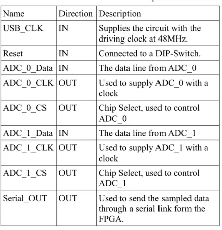
The FPGA implementation used four inputs and five outputs, seen in Table 4.1. These where used for the control the FPGA, the connected analog-to-digital converters and the connection to the FTDI circuit.

4.3.1 Reset_Debounce

Reset_Debounce, seen in Image 4.6, is used to reduce flicker when going from a reset state to an active state by requiring a logical one for three consecutive clock cycles ones to send out a '1' to the reset of the circuit. It's in- and out-puts are seen in Table 4.2.

Table 4.1: FPGA in- & out-puts

Name Direction Description

USB_CLK IN Supplies the circuit with the driving clock at 48MHz.

Reset IN Connected to a DIP-Switch.

ADC_0_Data IN The data line from ADC_0 ADC_0_CLK OUT Used to supply ADC_0 with a

clock

ADC_0_CS OUT Chip Select, used to control ADC_0

ADC_1_Data IN The data line from ADC_1 ADC_1_CLK OUT Used to supply ADC_1 with a

clock

ADC_1_CS OUT Chip Select, used to control ADC_1

Serial_OUT OUT Used to send the sampled data through a serial link form the FPGA.

(38)

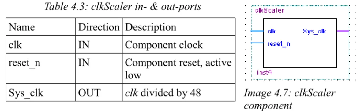
4.3.2 clkScaler

The clkScaler scales the 48MHz clock down to the 1MHz clock that is used for the rest of the system. Its block symbol can bee seen in Image 4.7 and its ports are described in Table 4.3.

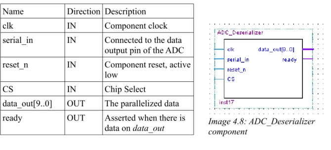
4.3.3 ADC_Deserializer

ADC_Deserializer is connected to the ADC an where responsible for reading the data sent by the ADC. There where one of these component for every ADC used to sample. ADC_Deserialiser is controlled through the CS signal. When CS goes low the component counts the two clock cycles that it takes for the ADC to sample, waits an additional cycle for the starting null bit and then starts to shift in the ten data bits sent by the ADC into a registry. Once it has received the ten data bits it sets the data_out port to the data and sets the ready port high to indicate that there is data on the bus. When CS goes high it returns to its idle state and waits for CS to go low again. The block diagram can be seen in Image 4.8 and the components port in Table 4.4.

Image 4.7: clkScaler component

Table 4.3: clkScaler in- & out-ports

clk IN Component clock

reset_n IN Component reset, active low

Sys_clk OUT clk divided by 48

Table 4.2: Reset_Debounce in- & out- ports

reset_n IN Component reset, active low

DB_reset_n OUT Debounced reset signal _{Image 4.6:}

Reset_Debounce component

(39)

4.3.4 Dual_ADC_Controller

Dual_ADC_Controller is the main component in the FPGA implementation, its block schematic can be seen in Image 4.9 and its ports are shown Table 4.5. It consists of three processes, the first one which controls when to sample and the second and third which together create a state machine that is used to read data from Data_1_in and Data_0_in and sends it in appropriate byte sizes to the transmiter2 component.

Image 4.8: ADC_Deserializer component

Image 4.9: Dual_ADC_Controller component

Table 4.4: ADC_Deserializer in- & out-ports

serial_in IN Connected to the data output pin of the ADC

reset_n IN Component reset, active

low

CS IN Chip Select

data_out[9..0] OUT The parallelized data

ready OUT Asserted when there is

data on data_out

Table 4.5: Dual_ADC_Controller in- & out-ports

ack IN Acknowledgement that

Data_out has been read

low

Data_1_in[9..0] IN Data line 1

Data_1_readable IN Assert to signal that there is data on Data_1_in Data_0_in[9..0] IN Data line 0

Data_0_readable IN Assert to signal that there is data on Data_0_in

CS OUT Chip Select

Data_out[7..0] OUT Data in byte size Data_available OUT Asserted when there is

(40)

The first process keeps track of the sample frequency by means of a counter. When sampling Dual_ADC_Controller desserts CS for 13 clock cycles, the time it takes for the ADC to sample and send the data, it then asserts CS again. The state machine generated by the second and third

processes waits for Data_0_readable and Data_1_readable to be asserted. It then reads the data from Data_0_in and Data_1_in and repackages the data into three bytes size packages. The data is then sent to the transmiter2 component by setting Data_out to the first byte and asserting

Data_Available. It then waits for ack to be asserted and then continues to do the same thing with

each of the remaining bytes.

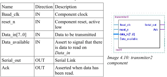
4.3.5 Transmiter2

Transmiter2 is a asynchronous one way serial UART. Port descriptions are shown in Table 4.6 and it block schematic can be seen in Image 4.10. When Data_available is asserted it reads data_in

asserts Ack and starts to send the data out through Serial_out following the regular serial communication used be serial ports with eight data bits, one stop bit and no parity bits. It then returns to waiting for Data_available to be asserted.

4.3.6 FTDI chip

The FT232RL chip that was used was supplied by Lars Asplund, our supervisor, and already fitted to a circuit board with a mini USB connection and ready pins for the serial communication with the FPGA. The FT232RL chip is produced by Future Technology Devices International Ltd. and is a USB to serial UART interface. It supports USB 2.0 full speed and a transmission frequency of 1MBaud over the serial connection. See [30] for additional information and the data sheet.

Image 4.10: transmiter2 component

Table 4.6: transmiter2 in- & out-ports

Baud_clk IN Component clock

low

Data_in[7..0] IN Data to be transmitted Data_available IN Assert to signal that there

is data to read on

Data_in

Serial_out OUT Serial Link

Ack OUT Asserted when data has

(41)

4.3.7 C#

To read the data read from the FPGA by the FTDI chip the manufacturers of the FTDI chip supplies drivers as well as C# wrapper classes for communication with the FTDI chip. These where used to configure the FTDI chip and and then the program attempts to continuously read from the chip. To avoid to much overhead over the USB connection 6000 bytes is read at a time for each read request. The byte sized data is reconstructed into the initial 10 bit values produced by the ADC and saved into two separate files. For the full code see Appendix J and for more information on the FTDI driver see [31].

4.4 Test sound 1

At first, the sound source consisted of sine waves with fixed frequencies and constant amplitude creating sounds as “ma”, “mat” and “mow” from [32]. It was shown early on that they did not give any useful results at all. The hypothesis for this is due to that the signals where harmonic and not fit for calculating the correlation. At higher frequencies it occurred that the delayed signal had its first top overlapping or going over the second not delayed signal as shown in Image 4.11.

This meant that the correlation is calculated on wrong period, creating abnormal result. To obtain accurate estimations and therefore avoiding overlapping the sound source can only be at angles between ± 11 degrees for frequencies at 1500 Hz. For future tests recordings of human speech was used which proved to give correct results.

(42)

The sound that instead is used is taken from a scene in the Swedish family comedy film “Sunes Sommar” from 1993. The scene takes place when Rudolf, the father of the main character, has in the search of coffee, ended up on the cashier side of the counter in an empty café. As he is about to drink his coffee a team of American basketball players enters the café, also on the search for coffee. When they have received their coffee they ask Rudolf what a pastry is called. The pastry in question is a chocolate ball or as it was often called during the early and mid ninety's, nigger ball. The

conversation that follows is the sound used and last around 13 seconds.

Rudolf: We call them ni-ni-n-n-nooo no no (smacks the table)NO! Rudolf: We call them w-weinerbröd.

Rudolf: Weinerbroads

Basketball player: Oh no you don't.

The sound wave can be seen in Image 4.12.

The recordings were made early in the morning when background noise was considered to be minimal. Only computer fans, ventilation and radiators are considered the only indoor sound sources. Some noise can also arise from outside the lab and the background noise where measured to 31 dB, while the sound was playing at ~60 dB measured between the microphone pair.

4.4.1 Dataset 1

In Dataset1 the sound source has been positioned at a distance of 1.5 meters and an elevation of 0.8 meters from the origin at different angles. The different angles are 90, 70, 60, 45, 35, 25, 15, 5, 0, -5, -15, -25, -35, -45, -60, -70, -90. Using first the omnidirectional microphones and then with the noise cancelling microphones. In total this equates to 34 paired recordings, 17 pairs with the

(43)

omnidirectional microphones and 17 pairs with the noise cancelling microphones generated by Test sound 1.

4.5 Algorithms

In this initial test the algorithms in use are rather basic and implemented in MATLAB. The four different algorithms for calculating the azimuth are constructed with MATLABs own cross-correlation function, MATLABs build-in Fourier transformation and iterative cross-spectrum function for omnidirectional and noise-cancelling microphones.

4.5.1 Matlab implementation 1 & 2

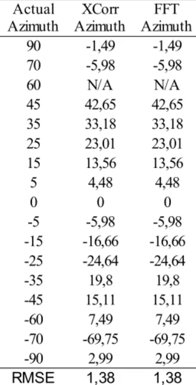
These algorithms uses the inbuilt functions of Matlab, xcorr(), fft() and ifft(), to estimate the azimuth. The first implementation only uses xcorr() to calculate the cross correlation while the second uses fft() to transform the signals into the frequency domain, calculate the CS and then using ifft() to transform the cross spectrum back into the time domain resulting in the cross correlation. The phase shift is then determined and used to calculate an estimation of azimuth. The Matlab code used can be found in Appendix I.

When the algorithms are used together with windowing, with 50 % overlap, the windows go through some additional calculations. First off, the mean energy is calculated for the window and compared to a threshold value. This is done to avoid making unnecessary calculations on

background noise. In the case of the FFT-implementation a Hanning window is applied to the windowed signal section make sure that it starts and stops at a value of zero. The xcorr-implementation is tested both with and without applying a Hanning window.

When using windowing there will be several azimuth estimations for the entire signal. To determine the just one azimuth the most frequent delay is chosen as a preliminary estimation. Then the mean is calculated from all nearby values.

(44)

4.5.2 Algorithm 1

The Algorithm 1 can be found in Appendix D and are a preparation algorithm, before calculating the cross-correlation. The algorithm centres the signals around zero, digitally filter both signals, divide them in chosen windows with 50 % overlap, check if the windowed signals have enough energy with mean energy function and at last apply a Hanning window function. After the process is finished the algorithm calls Algorithm 2 and receive an estimation of the discrete time delay. For Test – Initial test the cut-off frequency for the digital bandpass filter of 100-order is 300 to 8000 Hz, which give a sharp slope and can be found in Appendix D. The purpose of the digital filter is to filter unwanted signals received after the ADC. The window time is tested for 100, 50 and 25 milliseconds giving 2000, 1000 and 500 samples per window respectively. For Test – Initial test the result is represented by the median of all calculated windows of the entire signal. The threshold for mean energy where first tested with signals without sound and hence set to 500.

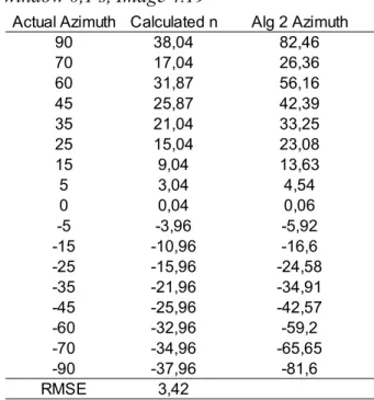
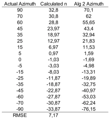
4.5.3 Algorithm 2

The inputs for Algorithm 2, which can be found in Appendix D, are the two received signals from the pair of microphones. The signals are transformed to the frequency domain using Fourier

transformation and are then used to iteratively calculate the CS. Variable t in Algorithm 2 is stepped to maximize variable sum based on equation 1.15. Variable t vary between negative to positive discrete time step corresponding -90 to 90 degree and due to that the omnidirectional and noise-cancelling microphones have different distance between them, variable t has different limit values. For omnidirectional microphones variable t vary between -38,37 to 38,37 and for noise-cancelling -34,88 to 34,88. The boundary values are calculated with equation 4.1.

rmax=±

distance∗sampling frequency

sound speed (4.1)

Sound localization for human interaction in real environment