Ray Tracing Non-Polygonal Objects: Implementation and Performance Analysis using Embree

(1)

Ray Tracing Non-Polygonal Objects:

Implementation and Performance

Analysis using Embree

Mälardalens University

School of Innovation, Design and Engineering Michael Carlie

Bachelor Thesis in Computer Science 2016-06-15

Examiner: Thomas Larsson Supervisor: Afshin Ameri

(2)

Abstract

Free-form surfaces and implicit surfaces must be tessellated before being rendered with rasterization techniques. However ray tracing provides the means to directly render such objects without the need to first convert into polygonal meshes. Since ray tracing can handle triangle meshes as well, the question of which method is most suitable in terms of performance, quality and memory usage is addressed in this thesis.

Bézier surfaces and NURBS surfaces along with basic algebraic implicit surfaces are implemented in order to test the performance relative to polygonal meshes

approximating the same objects. The parametric surfaces are implemented using an iterative Newtonian method that converges on the point of intersection using a bounding volume hierarchy that stores the initial guesses. Research into intersecting rays with parametric surfaces is surveyed in order to find additional methods that speed up the computation. The implicit surfaces are implemented using common direct

algebraic methods. All of the intersection tests are implemented using the Embree ray tracing API as well as a SIMD library in order to achieve interactive framerates on a CPU. The results show that both Bézier surfaces and NURBS surfaces can achieve interactive framerates on a CPU using SIMD computation, with Bézier surfaces coming close to the performance of polygonal counterparts. The implicit surfaces implemented outperform even the simplest polygonal approximations.

(3)

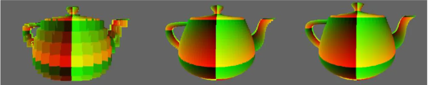
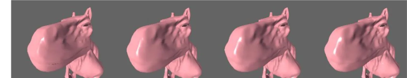
8. Results ... 41 8.1 Test System ... 41 8.2 Test Setup ... 41 8.3 Polygonal Meshes ... 42 8.3.1 Image Quality ... 42 8.3.3 Memory Consumption ... 43 8.4 Implicit Surfaces ... 43 8.4.1 Image Quality ... 43 8.4.2 Performance ... 44 8.4.3 Memory Consumption ... 46 8.5 Bézier Surfaces ... 46 8.5.1 Image Quality ... 46 8.5.2 Performance ... 47 8.5.3 Memory Consumption ... 49 8.6 NURBS ... 49 8.6.1 Image Quality ... 49 8.6.2 Performance ... 50 8.6.3 Memory Consumption ... 52 9. Discussion ... 52 9.1 Related Research ... 53 10. Conclusions ... 54 10.1 Future work ... 54 Bibliography ... 55

(5)

1. Introduction

Ray Tracing is a rendering technique that produces images by generating rays that are projected from the camera. Intersection tests are conducted between the rays and the geometry representations that constitute the scene in order to determine visibility and the amount of light that is reflected back along the rays towards the camera. Ray tracing is well suited for rendering photo-realistic images with reflections, refractions and other lighting techniques since the generated rays simulate the behavior of light. Geometry representations in rendering applications are typically represented using a set of adjacent polygonal faces that together represent the geometry. With ray tracing such polygonal meshes are rendered by conducting intersection tests with each of

the polygonal faces in the mesh, however ray tracing can also be used to render non-polygonal mathematically defined geometry representations. Many real-world objects can be represented using such mathematically defined geometries. Examples include implicit surfaces such as cones, cylinders ellipsoids and spheres, as well as Bézier surfaces and NURBS. Traditionally these geometries are approximated and represented using polygonal meshes in rendering applications through a process known as

tessellation, however such methods have problems with unintended artefacts and limited scalability.

1.1 Problem Definition

The ability to directly render non-polygonal geometry representations is useful for applications that need to circumvent the limitations of traditional polygonal meshes, however certain types of rendering applications, such as those that provide interactivity typically have performance constraints. Ray tracing implementations for various

geometry representations have varying complexity and resource usage which limits the types of geometry representations that might be suitable for applications with specific performance requirements. With this in mind the central questions that this paper will address are:

 Which non-polygonal geometry representations are suitable for usage in real-time ray tracing and how can they be implemented?

 How do various non-polygonal geometry representations compare with each other and their tessellated counterparts in terms of performance and resource usage?

2. Background

2.1 Rendering Algorithms

The fundamental algorithms used to represent images in computer graphics can be generally classified as either projective or image-space algorithms. Projective algorithms typically use a process known as rasterization to map the three-dimensional geometric representations to pixels in a two-dimensional space in a per object fashion. The shading of the individual objects is performed on each of the objects locally in order to give the appearance of depth and determine how they interact with light. Image-space

(6)

geometries along a line of sight and computing the amount of light that is reflected back towards the viewer for each pixel. A common type of image-space rendering algorithm is ray tracing [1].

Computer graphics implementations can be further categorized into offline and real-time implementations. The purpose of real-real-time rendering is to create the illusion of continuity in image rendering and providing interactivity by rapidly rendering each image based on the user’s input. This cycle of user input followed by rendering should happen at a fast enough rate to where the viewer is unaware of the fact that each image is rendered in a discrete fashion. The rate at which images are rendered and displayed is measured in frames per second (fps) or Hertz (Hz). Offline rendering implementations on the other hand are not necessarily concerned with the time it takes to render an image [2].

2.2 Ray Tracing

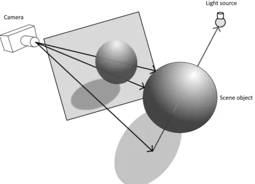
Ray tracing is an image-space based computer graphics technique first described by Whitted [3]. Ray tracing produces images by generating mathematical rays that are projected from the virtual camera in the scene. The rays are tested for intersection with each of the objects that constitute the scene in order to determine visibility and the amount of light that is reflected back along the rays towards the viewer.

The rays initially generated from the camera are called the primary rays. Secondary rays can be generated recursively from the points of intersection with objects in the scene of the primary rays in order to produce additional effects such as shadows, reflection and refraction. Rays can be successively generated from points of intersection of prior rays in order to increase realism or produce additional effects such as reflectivity. The

recursive generation can be halted based on some specified depth limit or when the rays stop producing significant information. The ray tracing algorithm is suitable for

(7)

Figure 1 A demonstration of the ray tracing algorithm with primary rays, shadow rays and a sphere object. Areas and objects under shadows are determined by generating a ray directed towards a light source from an initial point of intersection and testing for objects that are between the initial point of intersection and the light source If an object is detected by the

shadow ray the initial point of intersection is colored in such a way that it appears to be shaded. Reflection is determined by generating a reflected ray from a previous point of intersection on a reflective object and determining if there is another object in the path of the new reflection ray. If another object is detected the color of the point of

intersection of the original reflective object has the color of the object detected by the reflection ray added to it. [1]

A ray is represented mathematically by a point 𝒐 determining the ray’s origin, a vector 𝒅 representing the ray’s direction and a parameter 𝑡 where 𝑡 = 0 at the ray’s origin. Any point on the ray’s trajectory can be expressed as 𝑝 = 𝑜 + 𝑡𝑑.

2.2.1 Illumination

Once the visibility of an object in the scene has been determined a method is needed to determine what color the corresponding pixel should have. The simplest way to color an object is to simply assign some desired color to that pixel once a successful intersection test has been conducted. In order to give the appearance of being three-dimensional on a two dimensional screen an illumination model, simulating the way light interacts with physical objects, should be implemented. A common illumination model that simulates light was first described by Phong [4]. For each material in the scene the specular, diffuse, ambient and shininess constants, denoted 𝐾𝑠, 𝐾𝑑, 𝐾𝑎, 𝛼 respectively, are defined.

Additionally, we have L which is the direction from the point of intersection to the light point in the scene, the normal N from the surface at the point of intersection, R which is a vector representing the direction that a reflected ray originating from the light source would take if it hit the object at the point of intersection and V which is a vector pointing towards the camera from the point of intersection. The final color I then becomes

(8)

𝐼 = 𝐾_𝑎𝐼_𝑎+ 𝐾_𝑑𝐼_𝑑max(𝑁 ∙ 𝐿, 0) + 𝐾_𝑠𝐼_𝑠max ((𝑉 ∙ 𝑅)𝛼, 0) (4.51) Other lighting models for interesting effects and a more physically accurate modification

of the Phong model exist [5], however since the focus of this paper is on the intersection aspect of ray tracing, this basic illumination model is presented for a cursory

background on the subject of illumination.

2.3 Bounding Volume Hierarchy

A bounding volume hierarchy (BVH) is a set of volumes that bound each object in a scene and are arranged in a traversable tree structure. The root of the tree is a bounding volume that entirely encapsulates all objects in the scene with each successive node in the tree encapsulating a subset of smaller bounding volumes all contained within their parent node’s bounding volume. The leaf nodes of the tree finally bound single objects in the scene. Single objects can also be divided into a set of leaf nodes if their computation is expensive. A polygonal mesh may for example be divided into a bounding volume hierarchy so that each node contains a subset of the faces that constitute the mesh. With ray tracing the hierarchy is traversed by testing if the ray intersects each of the child volumes of each node and continuing down the tree from the node which the ray intersects. If the ray intersects several of the child nodes, then the one that is closest is traversed first. This way objects in the scene can be determined as not intersecting the ray since the ray does not intersect their bounding volume. Since ray tracing the objects directly is generally more expensive than ray tracing the bounding volume this tends to speed up the computation of each ray.

Various kind of bounding volumes can be used to construct such hierarchies. Spheres, bounding boxes and axis-aligned bounding boxes being the most common. The type of volume most suitable for the hierarchy usually depends on the types of objects

contained within the leaf nodes [6].

Other types of accelerated spacial structures exist such as uniform grids, bounding interval hierarchies, octrees and kd-trees. In [7] a comparative study of all of these types was conducted. The authors concluded that kd-trees are generally faster than bounding volume hierarchies but that bounding volume hierarchies have the advantage of lower memory consumption and a better availability of robust and fast building algorithms. Both kd-trees and bounding volumes hierarchies were faster than the other alternatives.

2.4 Embree

Embree is a CPU-based ray tracing API consisting of low-level kernels intended to maximize utilization of modern x86 CPU architectures using Single instruction, multiple data (SIMD) computation for ray traced rendering implementations. Embree allows for runtime code selection that optimizes the accelerated data structures, all of which are variant of bounding volume hierarchies, and build algorithms used in a way that best suits the hardware capabilities and architecture that the ray tracing implementation is running on. Both packet and single ray tracing intersection computations are supported with the ability to dynamically switch between them. Embree has built-in intersection methods for various primitives but also allows for user-defined intersection testing with arbitrary geometries [8].

(9)

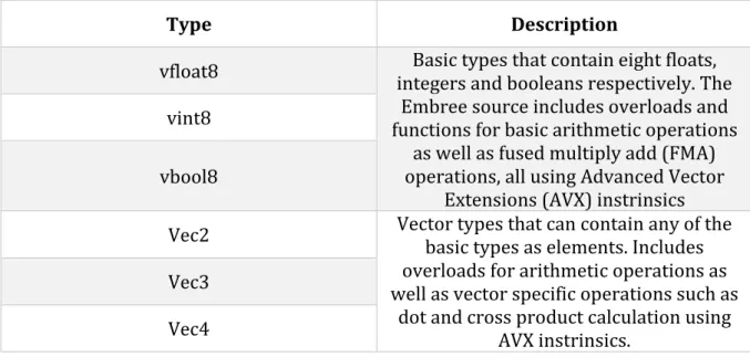
Embree supports ray packets of sizes 4, 8 or 16 for both determining intersection and occlusion. Embree also uses SIMD math library containing type definition for floating-point variables, double-precision variables, integers and booleans among others that can contain between 4 and 16 separate values in a SIMD variable which allows for

computing up to 16 simultaneous computations on each of the values in the variables. Besides these basic types the library also includes second, third and fourth dimensional vectors that can contain the respective variables in each of the elements allowing for easily implemented SIMD vector algebra computation. The SIMD library can be used for computing intersections with user defined geometries by including the library from the Embree source code, available at [9]. The following table described the types used in this thesis.

Table 1 The types from the Embree SIMD library used in this thesis

Type Description

vfloat8 _{integers and booleans respectively. The}Basic types that contain eight floats, Embree source includes overloads and functions for basic arithmetic operations

as well as fused multiply add (FMA) operations, all using Advanced Vector

Extensions (AVX) instrinsics vint8

vbool8

Vec2 Vector types that can contain any of the _{basic types as elements. Includes} overloads for arithmetic operations as well as vector specific operations such as

dot and cross product calculation using AVX instrinsics.

Vec3 Vec4

Embree uses a device concept, where an RTCDevice object is instantiated and used for each ray tracing system implemented in the code. These devises don’t interfere with each other so that several devices can be used for separate purposes. Embree also provides an RTCScene object which is a container for a list of geometries of potentially various types. Scenes can be created with different options depending on whether ray packets are supported or if the scene is to be dynamic or static.

For a dynamic scene, geometries that are included are enabled by default and can be disabled, re-enabled or removed. Once a geometry has been included in the scene and enabled a call to the API to commit the scene will cause a bounding volume hierarchy to be created for the objects in that particular scene. Objects can later be modified after which a subsequent call to commit the scene will cause the bounding volume hierarchy to be created again. On the other hand, a static scene cannot be modified after the initial call to commit the scene.

Each object that is placed in a scene is given a unique identification number called

geomID by Embree. This number can be used to retrieve, modify or delete the geometry once it’s in the scene.

(10)

The method with which Embree creates the bounding volume hierarchy for polygonal meshes can be altered by specifying one of the following flags when creating a scene. Table 2 Flags used to set the conditions for bounding volume hierarchy generation in Embree. The flags are considered suggestions by Embree and may be ignored

RTC_SCENE_COMPACT avoids algorithms that consume much Creates a compact data structure and memory.

RTC_SCENE_COHERENT Optimize for coherent rays (e.g. primary _rays). RTC_SCENE_INCOHERENT Optimize for in-coherent rays (e.g. diffuse _{reflection rays).} RTC_SCENE_HIGH_QUALITY Build higher quality spatial data _structures.

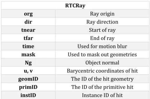
Embree also provides its own ray structures for various packet sizes that can be passed to a scene in order to check for intersection. The structure for a single ray is given in table 3.

Table 3 the ray object provided by Embree with a description of the associated types.

RTCRay

org Ray origin

dir Ray direction

tnear Start of ray

tfar End of ray

time Used for motion blur

mask Used to mask out geometries

Ng Object normal

u, v Barycentric coordinates of hit

geomID The ID of the hit geometry

primID The ID of the primitive hit

instID Instance ID of hit

For ray packets the data elements of the ray are eight length arrays of their single ray counterparts. The org, dir and Ng variables are split into three separated eight length arrays for each dimension for the ray packet structure.

The rays are passed to the scene by calling the function rtcIntersect for a single ray or rtcIntersect8 for a packet of eight rays along with the scene that the rays are going to be tested for intersection in. When calling an rtcIntersect function for a ray packet a valid mask also needs to be created and passed to the function. The valid mask is an integer array with each of the values initially set to negative one. When one of the rays in the ray packet intersects an object, Embree sets the corresponding element in the

(11)

valid mask to zero. When the packet is later tested against another object, any ray which has its valid mask set to zero is ignored. This also needs to be accounted for manually when implementing user geometries.

A list of geometries supported by Embree can be found at [10]. Embree uses the Möller-Trumbore method [11] for finding intersections between triangles and rays.

User geometries are created in Embree by providing a user created intersection and occlusion function. The functions are passed to Embree using the

rtcNewUserGeometry function which also accepts a pointer to the user data that is needed for performing the intersection tests. The user function receives the ray or ray packet and valid mask along with the user geometry and uses this information to fill the ray with data. The data that is passed to the ray is the geomID of the object that has been intersected, setting the tfar member of the ray to the intersection point and setting the normal values of the ray.

2.5 Non-Polygonal Ray Tracing

The popularity of rasterization techniques has caused polygonal meshes to become the geometry representation of choice. So much so that graphics hardware is often designed specifically for the efficient rendering of triangles. Non-polygonal geometry

representations generally have to be converted into polygonal meshes by tessellation techniques before rendering with rasterization software and hardware. Efficient tessellation techniques exist for NURBS and Bézier surfaces [12], as well as implicitly defined surfaces [13]. However, tessellation methods can cause artefacts to appear, increase memory usage and generally decrease the scalability and quality of the object that is approximated. Ray tracing on the other hand provides a method for the direct rendering of objects without the need for tessellation.

2.5.1 Ray Tracing Implicit Surfaces

Many methods exist for determining intersection with various forms of implicit surfaces. A comprehensive overview of various methods is given by Hart in [14].

Algebraic surfaces such as ellipsoids and cylinders can be formed into a polynomial function when combined with the equation of a ray. Surfaces such as spheres which form quadratic equations when represented as polynomial functions can be solved using the quadratic equation. Symbolic methods can also be used for finding roots of third and fourth degree polynomials however above that numerical methods need to be applied. An early attempt, mentioned by Hart, using Descartes rule of signs was implemented in [15] Interval analysis which is a numerical method for finding roots within error bounds was used by Mitchell [16]. LG-surfaces proposed by Karla and Barr [17] uses the

Lipschitz constants of the implicit function that guarantees finding the roots of the polynomial function where L gives the means to find the regions where a function f is guaranteed to not intersect the surface and G gives the directional derivative along the ray. Sphere tracing described by Hart in [18] marches along the ray towards the implicit surface in steps small enough that they are guaranteed not to miss the surface.

More recently real-time results were achieved using a marching algorithm by Singh and Narayanan. [19]. The method used can render algebraic implicit surface up to an order of 50 as well as non-algebraic surfaces at real-time rates on a GPU. Knoll et al. [20]

(12)

presented an algorithm based on interval arithmetic and affine transformation that reached interactive frame rates on both a CPU and GPU implementations using SIMD computation.

2.5.2 Ray Tracing Parametric Surfaces

Methods for determining ray intersections with free-form parametric surfaces such as Bézier surfaces and NURBS can be generally classified as either being based on iterative Newtonian methods or ones based on subdivision.

Initial methods for determining ray intersections with parametric surfaces were first presented by Kajiya [21] and Toth [22] Both employed different techniques based on iterative Newtonian methods in order to find the roots of the polynomial equations, with the former solving the problem of finding the initial values using direct algebraic

methods and the latter using interval analysis. In [23] Sweeny and Bartels presented a method for b-spline surfaces that preprocessed the surface into a structure of nested bounding boxes in order to find initial estimates. Martin et al. [24] presented a similar, faster iterative method, also using bounding boxes for initial estimates that focused on simplifying previous methods and presenting the method in a way more suitable for implementation. A further optimization is presented in [25] where only the derivatives of the rational function are calculated instead of both the non-rational and rational derivatives as in Martin’s method.

As for subdivision methods for ray tracing parametric surfaces; a method for

intersections with rational Bézier surfaces based on a technique called Bézier clipping was first introduces by Nishita, Sederbergt and Kakimoto in [26]. The technique takes advantage of the convex hull properties of Bézier and NURBS surfaces in order to iteratively remove sections that have not been intersected by the ray. Campagna,

Slusallek and Seidel in [27] presented an improved method based on Nishita’s algorithm. The method however requires NURBS surfaces to first be converted into simpler Bézier surfaces in order to work. In [28] the authors detail a problem with the original Bézier clipping method where multiple equivalent intersections can occur causing redundant computation and propose a method for reducing the probability of the phenomenon occurring.

Wang, Zen-Chung and Chuan [29] presented a method based on a combination of

Newtonian methods and Bézier clipping that uses ray coherence to find initial values for the Newtonian method. If that were to fail, then the algorithm instead adopts the Bézier clipping method as a substitution.

In [30] Abert, Geimer and Mulle take the recursive basis function for NURBS surfaces and converts it into a non-recursive form optimized for SIMD computation and uses the Newtonian method to find the roots. Several invariants in the surface evaluation are also pre-calculated and stored in a cache. The method was able to achieve greater than one frames per-second results on commodity hardware from 2006. Abert and Geimer also developed a SIMD based implementation for Bézier surfaces in 2005 [31] which

achieved between 3 – 5 frames per-second for various models. In a master’s thesis from 2010 [32] another implementation based on Newtonian methods with

bounding-volumes for initial value finding running on CUDA compatible GPUs achieved between 3-5 fps for various models, setups and techniques.

(13)

In [33] a third alternative for ray tracing parametric surfaces is presented. The method uses the second order derivative of the surface in order to find the roots of the surface equation with the ray. The method is able to better handle special cases than Newton’s method, such as the case where the ray intersects the surface at two points, however according the authors it takes longer to converge than Newton’s method.

3. Method

Initial research in this paper focuses on the various existing methods for representing objects and geometries without the usage of polygonal meshes in computer graphics. Specifically, the non-polygonal representations researched and implemented are ones for which there exist methods to determine ray-object intersections but are traditionally tessellated before rendering with rasterization. The geometry representations chosen for implementation are also constrained by feasibility of completion within the given time-frame of the thesis and the ability to implement with the tools used. The current or future practical usage in real-world implementations is also a discriminating factor. Methods for measuring common performance related quantities such as frames per second and relative scalability are developed in tandem with the intersection

implementations so that performance can be measured and compared. Literature on the subject is also evaluated in order to find other types of measurements that are

considered valuable given the context.

Embree is used for developing the respective implementations. The Embree API is used in order to remove the need for implementing custom accelerated structures and hardware parallelism. Embree has built in methods for ray tracing various geometry representations including polygonal meshes but also allows for user defined geometry representations that can use the accelerated structures and SIMD capabilities making it ideal for this work. Using an open source API rather than creating custom

implementations also provides an openly available and known point of comparison.

4. Theory

4.1 Implicit Surfaces

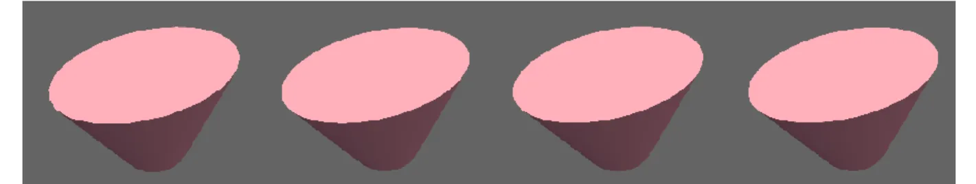
An implicit surface is a mathematically defined surface construct defined in three dimensions by an equation 𝑓(𝑥, 𝑦, 𝑧) = 0. In other words, an implicit surface is defined by the set of points (𝑥, 𝑦, 𝑧) that satisfy the condition 𝑓(𝑥, 𝑦, 𝑧) = 0.

Implicit surfaces can be used to represent a wide variety of surfaces. For example a plane as an implicit surface can be defined as 𝑥 + 𝑦 + 𝑧 = 0 and a sphere with radius

r can be defined as 𝑥2_{+ 𝑦}2_{+ 𝑧}2_{− 𝑟}2 _{= 0. Other examples include ellipsoids, cones, tori}

(14)

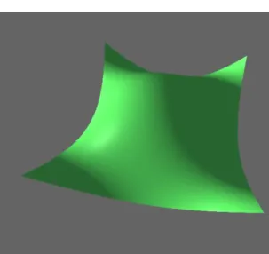
Figure 2 Implicit surfaces plotted with MATLAB’s isosurface function.

Implicit surface geometries can be bounded, i.e. occupying a finite amount of space such as in the case of a sphere, or unbounded such as the case of the plane where the surface extends into infinite space. The degree if an implicit surface is determined by the highest order variable in the defining polynomial, e.g. a sphere is a second degree or quadratic implicit surface since the highest degree for a single variable is two, and a torus is a fourth degree or quartic implicit surface since the highest degree for a single variable is four. Generally it is only possible to analytically solve implicit surfaces up to the fourth degree, beyond that alternative methods need to be applied [2].

4.2 Parametric Surfaces

A parametric equation assigns a parameter 𝑡 to each of the variables in an equation. As an example the equation of a circle with radius 𝑟 = 1 defined by 𝑥2_{+ 𝑦}2_{= 1 can}

parametrically be defined as

𝑆(𝑡) = {𝑥(𝑡) = cos(𝑡)

𝑦(𝑡) = sin(𝑡) (4.1)

Inserting a value for 𝑡 within the defined parametric interval 0 ≤ 𝑡 ≤ 1 will produce a point (𝑥, 𝑦) on the circle.

When dealing with three-dimensional parametric equations a second parameter value is introduces. The parametric equation for the sphere with radius 𝑟, otherwise defined by

𝑥2_{+ 𝑦}2_{+ 𝑧}2 _{= 𝑟} _(4.2) is defined parametrically as 𝑆(𝑢, 𝑣) = { 𝑥(𝑢, 𝑣) = 𝑟 ∙ sin(𝑢) ∙ cos(𝑣) 𝑦(𝑢, 𝑣) = 𝑟 ∙ cos(𝑢) ∙ cos(𝑣) 𝑧(𝑢, 𝑣) = 𝑟 ∙ sin(𝑣) (4.3) A set of two parameter values (𝑢, 𝑣) would then produce a point (𝑥, 𝑦, 𝑧) on the sphere.

In short, parametric surfaces are defined by taking the function of the surface and deriving a form of the function where each of the variables is defined by a couple of parameter variables (𝑢, 𝑣) which for any value within the defined interval produce a point on the surface.

(15)

𝑆(𝑢, 𝑣) = { 𝑥(𝑢, 𝑣) 𝑦(𝑢, 𝑣) 𝑧(𝑢, 𝑣) 𝑢 ∈ [𝑢_𝑚𝑖𝑛, 𝑢_𝑚𝑎𝑥], 𝑣 ∈ [𝑣_𝑚𝑖𝑛, 𝑣_𝑚𝑎𝑥] 4.3 Continuity

Continuity describes the differentiability or “smoothness” of a set of curves or surfaces. Continuity is written as 𝐶𝑛_{where 𝑛 is the amount of times that a set of curves are}

differentiable at a point. Some examples of levels of continuity including their geometric interpretation are.

𝐶−1: The curves are discontinuous, i.e. the curves don’t connect to each other. 𝐶0_{: The curves connect but the tangents differ at the points where they connect.}

𝐶1: There is a difference in acceleration at the points where the curves connect. 𝐶2: The point at which the curves connect have the same acceleration.

4.4 Bézier Curves and Surfaces

4.4.1 Bézier Curves

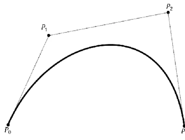
A Bézier curve is a polynomial curve that proportionally shapes itself relative to a set of control points. The curves can be a polynomial of any degree and a curve of degree 𝑛 will be controlled by 𝑛 + 1 control points. For computer graphics implementations it is common to approximate a shape using a set of connected cubic Bézier curves; such linear combinations of polynomials are called splines. The curve does not typically intersect the

individual control points of the curve, except for the beginning and ending control points, rather the curve is contained within the convex hull formed by the control points. The shape of the curve can be directly altered by manipulating the position of the individual control points making them ideal for computer aided design and modelling. A Bézier curve is written as

𝐶(𝑡) = ∑ 𝑃_𝑖𝐵_𝑖,𝑛(𝑡)

𝑛

𝑖=0

0 ≤ 𝑡 ≤ 1

(4.5)

Where 𝑛 is the degree of the curve, 𝑃_𝑖 are a set of two or three-dimensional control points, where the amount of control points is one more than the degree of the curve that they shape. 𝐵_𝑖,𝑛 are the blending functions of the curve defined as

Figure 3 A cubic Bézier curve with four control points

(16)

𝐵(𝑡)_𝑖,𝑛= 𝑛! 𝑛! (𝑛 − 𝑖)!𝑡

𝑖_{(1 − 𝑡)}𝑛−𝑖_{𝑖 = 0, … , 𝑛} _(4.6)

As an example, given two control points, 𝑃₀ and 𝑃₁, defining a linear or first degree curve, equation 4.5 expands to

𝐶(𝑡) = (1 − 𝑡)𝑃₀ + 𝑡𝑃₁

which is a finite straight line starting at 𝑃₀ and ending at 𝑃₁ given that 0 ≤ 𝑡 ≤ 1. If the control points are 𝑃₀, 𝑃₁, 𝑃₂, 𝑃₃ then the curve is cubic and is given by

𝐶(𝑡) = (1 − 𝑡)3𝑃₀ + 3𝑡(1 − 𝑡)2𝑃₁ + 3𝑡2(1 − 𝑡)𝑃₂ + 𝑡2𝑃₃

0 ≤ 𝑡 ≤ 1 (4.7)

with the terms

(1 − 𝑡)3

3(1 − 𝑡)2∗ 𝑡 3(1 − 𝑡) ∗ 𝑡2

𝑡2

(4.8) given by the blending functions for Bézier curves.

As can be seen a change in any of the control points results in a change of the entire curve; single Bézier curves are thus limited in the shapes that they can represent which means that a larger set of connected curves is required to represent closed shapes such as ellipsoids. However, limits also exist in the extent to which Bézier curves can be connected.

4.4.2 Continuity between Bézier Curves

Given two cubic curves with control points 𝑃₀, 𝑃₁, 𝑃₂, 𝑃₃ and 𝑄₀, 𝑄₁, 𝑄₂, 𝑄₃, simply setting the control points such that 𝑃₃ = 𝑄0 would create a composite curve or spline.

However merely placing the beginning and ending control points in the same place produces only 𝐶0_{continuity. In order to achieve 𝐶}1_{continuity, the following rule must}

be applied

𝑚(𝑃𝑚− 𝑃𝑚−1) = 𝑛(𝑄1− 𝑄0) (4.9)

Equation 4.9 entails that in order to achieve 𝐶1_{continuity between two connected}

Bézier curves the ratio of the distance between the last two control points of the first curve and the distance between the two control points of the second curve must be 𝑛/𝑚. Where 𝑚 is the degree of the first curve and 𝑛 is the degree of the second. Achieving 𝐶2

continuity or above is not possible for Bézier curves, although control points can always be positioned such that they at least appear to be continuous to a larger extent.

(17)

4.4.3 De Casteljau’s Algorithm

Finding a point on a Bézier curve given a parameter value 𝑡 can be achieved by simply inserting 𝑡 and doing the calculations as per the definition of Bézier curves. The problem with this method in terms of computation is that it is not very numerically stable. A more stable approach is given by De Casteljau’s algorithm [34].

The algorithm recursively linearly interpolates a point between each set of two adjacent control points until the desired value is found. Linearly interpolating a point 𝑡 ∈ [0,1] between two points 𝑃₀ and 𝑃₁ is done by

𝑃(𝑡) = 𝑃0(1 − 𝑡) + 𝑃1𝑡 (4.10)

The point 𝑃(𝑡) is then the point at parameter value 𝑡 along the line 𝑃₀ to 𝑃₁. The way that De Casteljau’s Algorithm works is that given a set of points 𝑃0, 𝑃1 … 𝑃𝑛. Linearly

interpolate a new point at 𝑡 along each successive pair of points 𝑃0 to 𝑃1 ... 𝑃𝑛−1 to 𝑃𝑛.

This gives a new set of n points. Continue the algorithm with the new set of points which gives another set of 𝑛 – 1 points. If done 𝑛 times, where 𝑛 is the degree of the curve, the result is a single point. This point is the point 𝑡 along the original curve.

The algorithm can be expressed with the following recursive equation

𝑃_𝑖,𝑗 = (1 − 𝑡)𝑃_{𝑖−1,𝑗}+ 𝑢𝑃_{𝑖−1,𝑗+1} {_{𝑗 = 0,1, … , 𝑛 − 𝑖}𝑖 = 0, 1, … , 𝑛 (4.11) Besides finding a point 𝑃(𝑡) on the curve, the algorithm can also be used to divide the

original curve at a point at 𝑡. The algorithm is simply applied at the split point 𝑡 until two new sets of control points can be retrieved which respectively describe both halves of the original curve.

An important note to make is that even though the convex hull property of the curve is always maintained when subdividing; the new control points will become closer and closer to the curve as higher levels of subdivision are applied, allowing for the creation of a successively tighter convex hull or control net.

4.4.4 Bézier Surfaces

A Bézier surface is formed by the product of the blending functions of two orthogonal Bézier curves. 𝑆(𝑢, 𝑣) = ∑ ∑ 𝑃𝑖,𝑗 𝑛! 𝑖! (𝑛 − 𝑖)!𝑢 𝑖_{(1 − 𝑢)}𝑛−𝑖 𝑚! 𝑗! (𝑚 − 𝑗)!𝑣 𝑗_{(1 − 𝑣)}𝑚−𝑗 𝑚 𝑗=0 𝑛 𝑖=0 0 ≤ 𝑢 ≤ 1 0 ≤ 𝑣 ≤ 1 (4.12) Or more compactly as 𝑆(𝑢, 𝑣) = ∑ ∑ 𝑃𝑖,𝑗𝐵𝑖,𝑛(𝑢)𝐵𝑗,𝑚(𝑣) 𝑚 𝑗=0 𝑛 𝑖=0 (4.13)

(18)

Like Bézier curves, Bézier surfaces are shaped by manipulating the associated control points and don’t generally intersect with the individual control points except for those situated on the corners of the surface. The surfaces are also contained within the convex hull formed by the control points. The same rules regarding continuity also apply. De Casteljau’s algorithm can be applied to a Bézier surface by applying it to each set of control points in both u and v direction.

4.4.5 Partial Derivatives

The derivatives of a Bezier surface have many uses such as finding the normal at a point or evaluating curvature. The partial derivatives in 𝑢 and 𝑣 direction are

𝐵𝑢(𝑢, 𝑣) = ∑ ∑ 𝑃𝑖,𝑗𝐵´𝑖,𝑛(𝑢)𝐵𝑗,𝑚(𝑣) 𝑚 𝑗=0 𝑛 𝑖=0 (4.14) 𝐵_𝑣(𝑢, 𝑣) = ∑ ∑ 𝑃_𝑖,𝑗𝐵_𝑖,𝑛(𝑢)𝐵´_𝑗,𝑚(𝑣) 𝑚 𝑗=0 𝑛 𝑖=0 (4.15)

The normal at the point (𝑢, 𝑣) can be found by normalizing the cross product of the two partial derivatives.

4.4.6 Matrix Representation

It is useful for many applications to represent a Bezier surface in matrix form. The way in which a cubic Bézier surface is represented as a matrix is described in [35] and will be outlined here.

A Bezier surface can be represented by the matrices

𝐵(𝑢, 𝑣) = [𝑈][𝑁][𝐶𝑃][𝑁]𝑇[𝑉]𝑇 _(4.16)

where for an 𝑛𝑡ℎ_{degree surface}

(19)

[𝑈] = [𝑢𝑛_𝑢𝑛−1_{… 1]}

[𝑉] = [𝑣𝑛_𝑣𝑛−1_{… 1]} (4.17)

[𝑁] is an (𝑛 + 1) by (𝑛 + 1) matrix containing the coefficients for the Bezier blending functions which for a cubic Bezier surface has the form

[𝑁] = [ −1 3 3 −6 −3 1 3 0 −3 3 1 0 0 0 0 0 ] (4.18)

The matrix [𝐶𝑃] contains the respective control points in both directions, making [𝐶𝑃] a (𝑛 + 1) by (𝑛 + 1) matrix of three-dimensional vectors.

[𝐶𝑃] = [ 𝑃0,0 𝑃0,1 𝑃_1,0 𝑃_1,1 𝑃0,2 𝑃0,3 𝑃_1,2 𝑃_1,3 𝑃_2,0 𝑃_2,1 𝑃_3,0 𝑃_3,1 𝑃_2,2 𝑃_2,3 𝑃_3,2 𝑃_3,3] (4.19)

The partial derivatives in both u and v direction can easily be represented in matrix form as 𝐵_𝑢(𝑢, 𝑣) = [𝑈´][𝑁][𝐶𝑃][𝑁]𝑇_[𝑉]𝑇 𝐵_𝑣(𝑢, 𝑣) = [𝑈][𝑁][𝐶𝑃][𝑁]𝑇_[𝑉´]𝑇 (4.20) where [𝑈´] = [𝑈𝑛−1_𝑈𝑛−2_{… 1 0]} [𝑉´] = [𝑉𝑛−1_𝑉𝑛−2_{… 1 0]} (4.21)

4.5 Non-Uniform Rational B-Spline (NURBS) Curves and Surfaces

4.5.1 NURBS Curve

Considering that non-uniform rational b-splines (NURBS) are the most general cases of b-splines it is beneficial to begin with the definition of b-splines and build towards the definition of NURBS more generally. B-spline or basis-spline curves are similar to Bezier curves in that they shape themselves relative to a set of control points. B-spline curves however offer increased flexibility over Bézier curves by allowing for piecewise

construction of several polynomial curves in a single spline construction. In other words, b-spline curves are not constrained by the 𝑛 + 1 control points rule for a 𝑛𝑡ℎ_degree

curve, but rather can increase the set of control points in order to increase flexibility and control as long as the number of control points are equal to or greater than the degree of the curve plus one. This increase in flexibility however entails an increase in

(20)

Besides the shape being determined by the set of control points and the degree, b-splines have an associated knot vector which defines the parameter intervals in which the control points provide local support and at which points the splines of a curve connect. Mathematically a b-spline curve is defined similarly to a Bezier curve by the polynomial

𝑓(𝑡) = ∑ 𝑃_𝑖

𝑛

𝑖=0

𝐵_𝑖(𝑡) (4.22)

Where 𝑃_𝑖 are the control points, 𝑛 is the number of control points and 𝐵_𝑖(𝑡) is the basis-function with respect to the parameter 𝑡.

Each of the individual control points can also have an associated weight 𝑤_𝑖. The weights can be increase in order for the associated control point to have an increased effect on the curve or decreased in order to reduce the effect on the curve. A b-spline with weights is defined by the polynomial

𝑓(𝑡) = ∑ 𝑤𝑖𝑃𝑖

𝑛

𝑖=0 𝐵𝑖(𝑡)

∑𝑛𝑖=0𝑤𝑖𝐵𝑖(𝑡)

(4.23)

A b-spline curve defined in such a way is called a rational curve given the rational form of the defining polynomial. In the case where all weights are equal to one, equation 4.23 reduces to equation 4.22, making the non-rational case a special case of the rational one. The weights of a b-spline curve must never be negative since that could break the

convex hull property of the curve. By multiplying the control points by the weights and appending the weights to the ends of each control point a more compact form of

equation 4.23 is

𝑓(𝑡) = ∑ 𝑃ℎ_𝑖

𝑛

𝑖=0

𝐵_𝑖(𝑡) (4.24)

Where 𝑃_𝑖ℎ_{denotes that the control points have had their weights appended and}

multiplied.

4.5.2 Basis Functions

The basis-functions that smoothly blend the curve given the set control points and parameter are given by the recursive Cox De-Boor formula defined by

𝐵_𝑖,0(𝑢) = {1 𝑖𝑓 𝑢𝑖 ≤ 𝑢 ≤ 𝑢𝑖+1

(21)

𝐵_𝑖,𝑝(𝑢) = 𝑢 − 𝑢𝑖

𝑢_𝑖+𝑝− 𝑢_𝑖𝐵𝑖,𝑝−1+

𝑢_𝑖+𝑝+1− 𝑢

𝑢_𝑖+𝑝+1− 𝑢_𝑖+1𝐵𝑖+1,𝑝−1(𝑢) (4.26) Here 𝑝 is the degree of the curve and 𝑖 is given by equation 4.23. As can be seen the

basis-functions are evaluated recursively starting from degree 𝑝 down to the 0th_degree,

meaning that for an increased degree the depth of the recursive formula increases and for an increase in control points the amount of basis-functions evaluated increases. The convention 0

0 = 0 is used. 𝑢𝑖 is the 𝑖

𝑡ℎ_{element of the curve’s knot vector.}

4.5.3 Knot Vector

The knot vector of a b-spline curve is defined by 𝑛 + 𝑝 + 1 elements where 𝑛 is the number of control points and 𝑝 is the degree. Mathematically the knot vector can be written as

𝑢⃗ = [𝑢0 𝑢1… 𝑢𝑛+𝑝] (4.27)

Each of the elements in the knot vector determine the points in the parameter domain at which the splines of the b-spline curve connect to each other or ‘tie-together’. The

minimum and maximum elements in a knot vector can be any number, including

negative ones, i.e. the magnitude of the vector does not matter. However, it is common to normalize the elements such that they are between zero and one. The elements in the knot vector must be set in a non-decreasing order, that is, 𝑢_𝑖 ≤ 𝑢_𝑖+1 for all elements in the knot vector meaning that [1 2 3 4 5 6] is a valid knot vector whereas [6 5 4 3 2 1] is not.

Each successive pair of elements in the knot vector 𝑢_𝑖 … 𝑢_𝑖+1 are referred to as a knot span and represent a particular parameter interval. The only valid knot spans are within the parameter domain 𝑢_𝑚𝑖𝑛 ≤ 𝑢 < 𝑢_𝑚𝑎𝑥 with 𝑢_𝑚𝑖𝑛 = 𝑢_𝑝 where 𝑝 is the degree of the curve and 𝑢_𝑚𝑎𝑥 = 𝑢_𝑛 where 𝑛 is the number of control points. Any parameter value outside of this span is not defined for the curve.

A non-empty knot span is any span where 𝑢𝑖 ≠ 𝑢𝑖+1. Such spans define a single

polynomial within the spline and therefore have 𝐶𝑝_{continuity within that span, where 𝑝}

is the degree of the curve. Increasing the number of equal knots in a knot span to some number produces an empty knot span and increases that span’s multiplicity. Increasing multiplicity decreases the differentiability or continuity of the basis-functions defined by the span to 𝐶𝑝−𝑘_{where 𝑝 is the degree and 𝑘 is the multiplicity. As an example, take a}

cubic curve with four control points and multiplicity k = 4

𝑢⃗ = [0 0 0 0 ⏞ 𝑘=4 1 1 1 1 ⏞ 𝑘=4 ] (4.28)

The valid knot span of this curve is 𝑢₃ ≤ 𝑢 < 𝑢₄. So 𝑢 is defined between 0 and 1 with a single polynomial curve of 𝐶𝑝_{continuity. In fact, if setting all of the weights to one for}

(22)

If we instead take a cubic curve with five control points and the knot vector 𝑢⃗ = [0 0 0 0 ⏞ 𝑘=4 0.5⏞ 𝑘=1 1 1 1 1 ⏞ 𝑘=4 ] (4.29)

Then we have a spline defined by two polynomial curves the first of which is defined within the parameter 𝑢1 ∈ [0, 0.5] and the second 𝑢2 ∈ [0.5, 1]. The two polynomial

curves meet at the point 𝑢 = 0.5 and have 𝐶𝑝−𝑘 _{= 𝐶}2_{continuity at that point.}

Increasing the multiplicity of the middle knot element would decrease the continuity at that point but would also necessitate increasing either the degree (which would

consequently make the continuity unaltered) or increasing the number of control points. Increasing the degree may change the shape of the curve so it is necessary to increase the amount of control points if maintaining the original form is required. The process of inserting new knots into a knot vector while maintaining the same original shape is called knot insertion, described in more detail in section 4.4.5

Knot vectors can be classified into three different types: uniform, open uniform and non-uniform.

Uniform knot vectors are knot vectors for which the spacing between each of the elements is equal. An example would be [0 1 2 3 4 5 6] or [0 0.1 0.2 0.3 0.4 0.5 0.6]. Uniform knot vectors can be used to describe closed shapes by making the endpoints coincide.

An open uniform knot vector has equidistant knots except for the beginning and ending knots which have multiplicity 𝑝 + 1 where 𝑝 is the degree of the curve. An example of an open uniform curve would be [0 0 0 0 0.25 0.5 0.75 1 1 1 1] for a cubic spline with seven control points.

Lastly, non-uniform knot vectors are the most general form of knot vectors where the only constraint is that the elements of the knot vector are in ascending order. Both uniform and open uniform knot vectors are special cases of non-uniform knot vectors. 4.5.4 Local Support

It follows from equation 4.25 and 4.26 that any basis function 𝐵_𝑖,𝑝(𝑡) is non-zero only within the knot span [𝑡_𝑖, … , 𝑡_𝑖+𝑝+1]. This property is referred to as local support which leads to the property of local modification which says that a control point 𝑃_𝑖 only has an effect on the curve within the interval [𝑡_𝑖, … , 𝑡_𝑖+𝑝+1], which allows the curve to be modified within a certain parameter interval without the rest of the curve being affected. The parameter intervals in which specific control points or sets of control points have an effect on the curve is determined by the knot vector.

4.5.5 Knot Insertion

It is possible to insert new knots into a knot vector while maintaining the original shape and increasing the amount of control points. Knot insertion is not only useful for

allowing a higher degree of fine tuning, but also finds use in subdivision algorithms. Given a b-spline curve defined by

(23)

𝑓(𝑡) = ∑ 𝑃_𝑖

𝑛

𝑖=1

𝐵_𝑖(𝑡) (4.30)

and knot vector

𝑢⃗ = [𝑢0 𝑢1… 𝑢𝑙 𝑢𝑙+1… ] (4.31)

Inserting a new knot between 𝑢𝑙 and 𝑢𝑙+1 gives the new curve

𝑓(𝑡) = ∑ 𝑄_𝑖

𝑛+1

𝑖=1

𝐵_𝑖(𝑡) (4.32)

Where the new control points 𝑄𝑖 are given by

𝑄_𝑖 = (1 − 𝛼_𝑖)𝑃_𝑖−1+ 𝛼_𝑖𝑃_𝑖 (4.33) 𝛼_𝑖 = { 1 𝑖 ≤ 𝑙 − 𝑘 + 1 0 𝑖 ≥ 𝑙 + 1 𝑢̅ − 𝑢_𝑖 𝑢𝑙+𝑘−1− 𝑢𝑖 𝑙 − 𝑘 + 2 ≤ 𝑖 ≤ 𝑙 (4.34)

where 𝑢̅ is the new knot and 𝑘 is the order of the curve, i.e. the degree of the curve plus one. Although the new curve has a different knot vector and different set of control points, it is geometrically equivalent to its previous shape. The algorithm for inserting one knot at a time is known as Boehm’s algorithm [36]. A more general form that handles the insertion of multiple knots simultaneously is known as the Oslo algorithm [37], [38] which is briefly detailed here.

Given a knot vector

𝑢⃗ = [𝑢₀ 𝑢₁… 𝑢_𝑛+𝑝+1] (4.35)

Inserting an arbitrary amount of new knots will give the new knot vector

𝑣 = [𝑣₀ 𝑣₁… 𝑣_𝑚+𝑝+1] (4.36)

Where 𝑚 > 𝑛 and corresponds to the number of inserted knots. The new curve is then defined by

(24)

𝑔(𝑡) = ∑ 𝑄_𝑗ℎ

𝑚

𝑗=0

𝐵_𝑗(𝑡) (4.37)

Since the new curve is geometrically equivalent to the previous one, the new control points can be computed based on the identity 𝑓(𝑡) = 𝑔(𝑡) where 𝑓(𝑡) is the old curve defined by the knot vector 𝑢⃗ . With this in mind; the new control points are derived using the equations. 𝑄_𝑗ℎ = ∑ 𝑃_𝑗ℎ 𝑚 𝑖=0 𝛼_𝑖,𝑗𝑝 (4.38) 𝛼_𝑖,𝑗0 = {1 𝑢𝑖 ≤ 𝑣𝑗 ≤ 𝑢𝑖+1 0 𝑜𝑡ℎ𝑒𝑟𝑤𝑖𝑠𝑒 (4.39) 𝛼_𝑖,𝑗𝑝 = 𝑣𝑖+𝑝− 𝑢𝑖 𝑢𝑖+𝑝 − 𝑢𝑖 𝛼_𝑖,𝑗𝑝−1+𝑢𝑖+𝑝−1− 𝑣𝑗+𝑝 𝑢𝑖+𝑝−1− 𝑢𝑖+1 𝛼_𝑖+1,𝑗𝑝−1 _(4.40) 4.5.6 NURBS Surface

A NURBS surface is created by the tensor product of two NURBS curves 𝑆(𝑢, 𝑣) = ∑ ∑ 𝐵𝑖,𝑝(𝑢)𝐵𝑗,𝑞(𝑣)𝑃𝑖,𝑗𝑤𝑖,𝑗 𝑚 𝑗=0 𝑛 𝑖=0 ∑ ∑𝑚 𝐵_𝑖,𝑝(𝑢)𝐵_𝑗,𝑞(𝑣)𝑤_𝑖,𝑗 𝑗=0 𝑛 𝑖=0 (4.41) Where p, and q are the respective degrees of the curves. Each curve in the construction

has a separate knot vector and can therefore each have a separate number of control points. A more succinct form of the equation where the weights have been appended to and multiplied with the control points is

𝑆(𝑢, 𝑣) = ∑ ∑ 𝐵_𝑖,𝑝(𝑢)𝐵_𝑗,𝑞(𝑣)𝑃_𝑖,𝑗ℎ 𝑚 𝑗=0 𝑛 𝑖=0 (4.42) All of the properties associated with NURBS curves, such as the convex hull property and

(25)

4.5.7 Partial Derivatives

The derivatives of a NURBS surface can be used for finding the normal at a point or evaluating curvature among other useful properties. In order to find the derivative of the NURBS surface the numerator and denominator are represented as separate functions as follows 𝑆(𝑢, 𝑣) = ∑ ∑ 𝐵𝑖,𝑝(𝑢)𝐵𝑗,𝑞(𝑣)𝑃𝑖,𝑗𝑤𝑖,𝑗 𝑚 𝑗=0 𝑛 𝑖=0 ∑𝑛_𝑖=0∑𝑚_𝑗=0𝐵_𝑖,𝑝(𝑢)𝐵_𝑗,𝑞(𝑣)𝑤_𝑖,𝑗 = 𝑁(𝑢, 𝑣) 𝐷(𝑢, 𝑣) (4.43)

The quotient rule can then be applied which produces

𝑆_𝑢(𝑢, 𝑣) = 𝐷(𝑢, 𝑣)𝑁𝑢´(𝑢, 𝑣) − 𝑁(𝑢, 𝑣)𝐷𝑢´(𝑢, 𝑣)

[𝐷(𝑢, 𝑣)]2 (4.44)

𝑆_𝑣(𝑢, 𝑣) = 𝐷(𝑢, 𝑣)𝑁𝑣´(𝑢, 𝑣) − 𝑁(𝑢, 𝑣)𝐷𝑣´(𝑢, 𝑣)

[𝐷(𝑢, 𝑣)]2 (4.45)

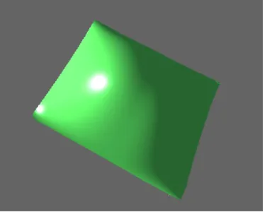
Which are the partial derivatives of a NURBS surface in both u and v direction where 𝑁_𝑢´(𝑢, 𝑣) = ∑ ∑ 𝐵´_𝑖,𝑝(𝑢)𝐵_𝑗,𝑞(𝑣)𝑃_𝑖,𝑗𝑤_𝑖,𝑗 𝑚 𝑗=0 𝑛 𝑖=0 (4.46) 𝑁𝑣´(𝑢, 𝑣) = ∑ ∑ 𝐵𝑖,𝑝(𝑢)𝐵´𝑗,𝑞(𝑣)𝑃𝑖,𝑗𝑤𝑖,𝑗 𝑚 𝑗=0 𝑛 𝑖=0 (4.47) Figure 5 A cubic NURBS surface with 20 control points, 5 in

(26)

𝐷_𝑢´(𝑢, 𝑣) = ∑ ∑ 𝐵´_𝑖,𝑝(𝑢)𝐵_𝑗,𝑞(𝑣)𝑤_𝑖,𝑗 𝑚 𝑗=0 𝑛 𝑖=0 (4.48) 𝐷_𝑣´(𝑢, 𝑣) = ∑ ∑ 𝐵_𝑖,𝑝(𝑢)𝐵´_𝑗,𝑞(𝑣)𝑤_𝑖,𝑗 𝑚 𝑗=0 𝑛 𝑖=0 (4.49)

and the derivative of the basis function is given by

𝐵´_𝑖,𝑝(𝑡) = 𝑝

𝑡_𝑖+𝑝− 𝑡_𝑖𝐵𝑖,𝑝−1(𝑡) −

𝑝

𝑡_𝑖+𝑝+1− 𝑡_𝑖+1𝐵𝑖+1,𝑝−1(𝑡) (4.50)

Note that 𝐵𝑖,𝑝−1(𝑡) and 𝐵𝑖+1,𝑝−1(𝑡) in equation 4.50 refer to the original Cox De-Boor

recurrence and not the derivative, i.e. the recursion continues down the original basis function where only the first layer is changed to the equation 4.50.

5 Ray Tracing Implicit Surfaces

5.1 Ray-Sphere Intersection

A common method for finding the point of intersection between a ray and a sphere is given in [39]. The sphere is defined by the center 𝑐, radius 𝑟 and a point 𝑝 on the sphere by

(𝑝 − 𝑐)2_{− 𝑟}2_{= 0} _(5.1)

To determine a point of intersection the point 𝑝 is substituted with the ray equation

(𝑜 + 𝑡𝑑 − 𝑐)2_{− 𝑟}2 _{= 0} _(5.2)

Expanding equation 5.2 gives

(𝑑2_)𝑡2_{+ 2𝑑𝑡(𝑜 − 𝑐) + (𝑜 − 𝑐)}2_{− 𝑟}2_{= 0} _(5.3)

Which is a quadratic equation for t that can be written as 𝑎𝑡2_{+ 𝑏𝑡 + 𝑐 = 0}

𝑎 = 𝑑2 𝑏 = 2𝑑(𝑜 − 𝑐) 𝑐 = (𝑜 − 𝑐)2 − 𝑟2

(27)

the solution for the equation is

𝑡 =−𝑏 ± √𝑏

2_{− 4𝑎𝑐}

2𝑎

(5.5) Quadratic equations have zero, one or two roots which can be determined by the

discriminant

𝑏2 − 4𝑎𝑐 (5.6)

If the value of the discriminant is less than zero then the ray does not intersect the sphere, if the discriminant is equal to zero then the ray grazes the sphere at a single point and if the discriminant is greater than zero then the ray goes through the sphere. Two points of intersection can then be determined from the equation; one where the ray enters the sphere and one where it exits. The point nearest the camera becomes the point used for determining the color of the corresponding pixel on the screen.

5.2 Ray-Cylinder Intersection

The equation for an infinite cylinder oriented along the line 𝑐 = 𝑜_𝑐+ 𝑡_𝑐𝑑_𝑐 with radius 𝑟 is given by

(𝑞 − 𝑜_𝑐− ((𝑑_𝑐∙ 𝑞 − 𝑜_𝑐) ∙ 𝑑_𝑐)2 = 𝑟2 (5.7)

where 𝑞 = (𝑥, 𝑦, 𝑧) is a point on the curve. Substituting the point with the ray equation 𝑞 = 𝑜 + 𝑡𝑑, the cylinder equation can be transformed into the quadric form 𝑎𝑡2_{+ 𝑏𝑡 +}

𝑐 = 0 where 𝑎 = (𝑑 − (𝑑 ∙ 𝑑𝑐) ∙ 𝑑𝑐)2 𝑏 = 2((𝑑 − (𝑑 ∙ 𝑑_𝑐)) ∙ ((𝑜 − 𝑜_𝑐) − ((𝑜 − 𝑜_𝑐) ∙ 𝑑_𝑐)𝑑_𝑐) 𝑐 = ((𝑜 − 𝑜𝑐) − ((𝑜 − 𝑜𝑐) ∙ 𝑑𝑐)𝑑𝑐) 2 − 𝑟2 (5.8)

The solution to the equation is given by

𝑡 =−𝑏 ± √𝑏

2_{− 4𝑎𝑐}

2𝑎 (5.9)

where a non-negative discriminant

𝑏2 − 4𝑎𝑐 ≥ 0 (5.10)

entails that the ray intersects the cylinder. In order to have a finite cylinder the ray is tested to see if it between the two planes determined by the line around which the

(28)

cylinder revolves by

𝑑_𝑐∙ (𝑞 − 𝑜_𝑐) > 0 𝑑_𝑐∙ (𝑞 − 𝑐) < 0

(5.11)

Where 𝑞 is the ray equation with 𝑡 set to the point of intersection and 𝑐 is the line that the cylinder revolves around with 𝑡_𝑐 set to the length of the cylinder.

Rendering a closed cylinder requires testing for intersection with the planes that bound the cylinder. The equations for planes contained within the cylinder’s radius 𝑟 are given by

𝑑𝑐 ∙ (𝑞 − 𝑜𝑐) = 0 𝑎𝑛𝑑 (𝑞 − 𝑜𝑐)2 < 𝑟2

𝑑_𝑐∙ (𝑞 − 𝑐) = 0 𝑎𝑛𝑑 (𝑞 − 𝑐)2 _{< 𝑟}2

(5.12)

Finding the final point of intersection is done by retrieving the non-negative results from equation 5.9 and the non-negative results from equations 5.12 The smallest of these values then determines the point of intersection [40].

6. Ray Tracing Parametric Surfaces

The Newtonian method for finding an intersection with a ray and both NURBS surfaces and Bézier surfaces differs only in the surface evaluation. Therefore, this section is dedicated to detailing the aspects of the intersection method that both types of surfaces have in common. The differences will be detailed in their respective dedicated sections. The Newtonian method for ray tracing parametric surfaces described here is based on the methods described by Martin in [24] with the additional enhancement developed by Abert [30].

6.1 Newton Rhapson

The Newton-Rhapson method, is an iterative method for finding the roots of a function. Given an initial guess, a function and its derivative; the Newton method for a function of a single variable is as follows

𝑥₁ = 𝑥₀− 𝑓(𝑥0)

𝑓´(𝑥₀) (6.1)

Where 𝑥₀ is the initial guess and 𝑥₁ is a new value for 𝑥 closer to the root given that the iteration converged towards the root.

(29)

𝑥_𝑖+1= 𝑥_𝑖− 𝑓(𝑥𝑖)

𝑓´(𝑥_𝑖) (6.2)

With a good initial guess the rate of convergence is quadratic. However, a bad guess or local extrema may cause the iteration to diverge from the root.

6.2 Ray Representation

The ray for which an intersection with the surface is to be found is normally represented by the equation

𝑟 = 𝑜 + 𝑡𝑑 (6.3)

Using a technique developed by Kajiya [21] for the Newtonian method, the ray is instead represented as the intersection of two orthogonal planes each represented as 𝑝1 =

(𝑛₁, 𝑑₁) and 𝑝₂ = (𝑛₂, 𝑑₂) where 𝑛₁ and 𝑛₂ are two unit length vectors that are

orthogonal to each other and 𝑑1, 𝑑2 represent the distance of each plane to the origin.

The original ray representation can be transformed into the two planes by applying the following

𝑛1 = {

(𝑑_𝑦, −𝑑_𝑧, 0) 𝑖𝑓 |𝑑_𝑥| > |𝑑𝑦| 𝑎𝑛𝑑 |𝑑𝑥| > |𝑑𝑧|

(0, 𝑑_𝑧− 𝑑_𝑦) 𝑜𝑡ℎ𝑒𝑟𝑤𝑖𝑠𝑒 (6.4) Applying the above rule causes 𝑛1 to always be perpendicular to the ray direction 𝑑. 𝑛2

can then simply be retrieved by

𝑛2 = 𝑛1× 𝑑 (6.5)

and the respective distances are given by

𝑑1 = −𝑛1∙ 𝑜

𝑑2 = −𝑛2∙ 𝑜 (6.6)

6.3 Newton’s Method for Ray-Surface Intersection

Finding the intersection between a ray and a surface turns into the problem of finding the roots for the bivariate equation

𝑅(𝑢, 𝑣) = {𝑛1∙ 𝑆(𝑢, 𝑣) + 𝑑1

𝑛2∙ 𝑆(𝑢, 𝑣) + 𝑑2 (6.7)

Where 𝑆(𝑢, 𝑣) is the point given by evaluating either the NURBS surface or the Bézier surface at a point in terms of 𝑢 and 𝑣. In geometric terms |𝑅(𝑢, 𝑣)| can be interpreted as the distance between the ray and the evaluated surface point 𝑆(𝑢, 𝑣). Since the

(30)

Newtonian method iteratively approximates the roots, an intersection is reported once the distance comes under a certain user defined threshold

|𝑅(𝑢, 𝑣)| < 𝜀 (6.8)

The iteration is stopped whenever any new u, v values given from the iteration results in a point further away from the ray

|𝑅(𝑢𝑖+1, 𝑣𝑖+1)| > |𝑅(𝑢𝑖, 𝑣𝑖)| (6.9)

Lastly no intersection is reported if the number of Newton iterations surpasses some user defined threshold.

Finding the new 𝑢, 𝑣 values given the old ones is done by applying

(𝑢𝑖+1 𝑣_𝑖+1) = (

𝑢_𝑖 𝑣_𝑖) − 𝐽

−1_{𝑅(𝑢, 𝑣)} _(6.10)

J is known as the Jacobian matrix and is given by

𝐽 = (𝑛1∙ 𝑆𝑢(𝑢, 𝑣) 𝑛1∙ 𝑆𝑣(𝑢, 𝑣) 𝑛₂∙ 𝑆_𝑢(𝑢, 𝑣) 𝑛2∙ 𝑆𝑣(𝑢, 𝑣) ) (6.11) and 𝐽−1 ₌ 1 det (𝐽)( 𝑛2∙ 𝑆𝑣(𝑢, 𝑣) −𝑛1∙ 𝑆𝑣(𝑢, 𝑣) −𝑛2∙ 𝑆𝑢(𝑢, 𝑣) 𝑛1∙ 𝑆𝑢(𝑢, 𝑣) ) (6.12) det(𝐽) = (𝑛₁∙ 𝑆_𝑢(𝑢, 𝑣)) ∗ (𝑛₂ ∙ 𝑆_𝑣(𝑢, 𝑣)) − (𝑛₂∙ 𝑆_𝑢(𝑢, 𝑣)) ∗ (𝑛₁∙ 𝑆_𝑣(𝑢, 𝑣)) (6.13) Equation 6.10 is as can been seen analogous to the Newton Rhapson formula (equation

6.2)

A problem, noted in [24], may arise if the determinant det(𝐽) is singular, i.e. det(J) ≈ 0. Such a determinant may make it difficult to determine the inverse Jacobian. The

problem can be circumvented by performing a small random perturbation of the 𝑢, 𝑣 values after checking if the Jacobian is near zero and initiating the next iteration if it is.

(𝑢𝑖+1 𝑣_𝑖+1) = ( 𝑢𝑖 𝑣_𝑖) + 0.1 ∗ ( 𝑟𝑎𝑛𝑑(0,1) ∗ (𝑢0− 𝑢𝑖) 𝑟𝑎𝑛𝑑(0,1) ∗ (𝑣₀− 𝑣_𝑖) ) (6.14)

(31)

Where 𝑢₀ and 𝑣₀ are the initial guesses and 𝑟𝑎𝑛𝑑(0,1) produces a random value between 0 and 1.

Since the final point retrieved is an approximation and most likely does not lie on the ray’s path a projection of the point onto the ray is performed using

𝑡 = (𝑆(𝑢, 𝑣) − 𝑜) ∙ 𝑑 (6.15)

6.4 Bézier Surface Evaluation

Evaluating a point on a bicubic Bézier surface given a set of 𝑢, 𝑣 values becomes an easier task if the surface is represented in matrix form [31] by

𝑆(𝑢, 𝑣) = [𝑈][𝑁][𝐶𝑃][𝑁]𝑇[𝑉]𝑇 _(6.16)

As previously mentioned, [𝑈] and [𝑉] are [𝑢𝑛_𝑢𝑛−1_{… 1] and [𝑣}𝑛_𝑣𝑛−1_{… 1] respectively,}

[𝑁] contains the polynomial coefficients and [𝐶𝑃] is a 4x4 matrix of three-dimensional vectors.

Since the product [𝑁][𝐶𝑃][𝑁]𝑇_{only ever changes when the control points change, it can}

be computed during the preprocessing step and stored in a separate matrix. It’s also worth noting that as long as [𝑈] and [𝑉] are represented in the order described where the elements start from 𝑢𝑛_{to 1 then [𝑁] is equal to its transpose [𝑁]}𝑇_{and therefore the}

transpose need not be calculated.

The surface evaluation begins with the calculation of [𝑈], [𝑉], [𝑈´], and [𝑉´]. After which the products [𝑈][𝑁][𝐶𝑃][𝑁]𝑇_{and [𝑈´][𝑁][𝐶𝑃][𝑁]}𝑇_{are determined. The calculation then}

continues for [𝑈][𝑁][𝐶𝑃][𝑁]𝑇_{[𝑉], [𝑈´][𝑁][𝐶𝑃][𝑁]}𝑇_{[𝑉] and [𝑈][𝑁][𝐶𝑃][𝑁]}𝑇_[𝑉´]

Doing the calculation of both the point on the surface as well as the partial derivatives in the same scope allows for the product [𝑈][𝑁][𝐶𝑃][𝑁]𝑇_{to be pre-calculated and used for}

the calculation of [𝑈][𝑁][𝐶𝑃][𝑁]𝑇_{[𝑉] and [𝑈][𝑁][𝐶𝑃][𝑁]}𝑇_{[𝑉´] considering the products}

that they have in common which decreases the amount of calculations needed compared with doing the surface evaluation for the point and the derivatives separately.

The results of these calculations are three three-dimensional vectors representing the point of the surface corresponding to the given 𝑢, 𝑣 values and the partial derivatives in 𝑢 and 𝑣 direction respectively.

6.5 Bézier Surface Subdivision

In order to create the bounding volume hierarchy for Bézier surfaces, the surface needs to be successively subdivided until a certain flatness criterion is met. De Casteljau’s Algorithm (described in section 4.3.3) can be used for successively subdividing a Bézier surface at a parameter value 𝑡. The algorithm is applied to each of the curves that

compose the surface in a single direction. The following shows how to subdivide a cubic Bézier curve at 𝑡 = 0.5.

(32)

𝑃(𝑡) = 𝑃₀(1 − 𝑡) + 𝑃1𝑡 (6.17)

Which for 𝑡 = 0.5 simplifies to

𝑃(𝑡) = (𝑃0 + 𝑃1) ∗ 0.5 (6.18)

Given the original four control points 𝑃0, 𝑃1, 𝑃2, 𝑃3 and parameter t = 0.5. A new set of

linearly interpolated points 𝑄0, 𝑄1, 𝑄2 is given by

𝑄₀ = (𝑃₀+ 𝑃₁) ∗ 0.5 𝑄1 = (𝑃1+ 𝑃2) ∗ 0.5

𝑄2 = (𝑃2+ 𝑃3) ∗ 0.5

(6.19)

Finally, these points along with the original points are used to construct the final set of 2n + 1 points 𝑅0, 𝑅1, 𝑅2, 𝑅3, 𝑅4, 𝑅5, 𝑅6 by 𝑅₀ = 𝑃₀ 𝑅₁ = 𝑄₀ 𝑅₂ = (𝑄₀+ 𝑄₁) ∗ 0.5 𝑅₄ = (𝑄₁+ 𝑄₂) ∗ 0.5 𝑅₃ = (𝑅₂+ 𝑅₄) ∗ 0.5 𝑅₅ = 𝑄₂ 𝑅₆ = 𝑃₃ (6.20)

Which produces the new pair of curves 𝑅0, 𝑅1, 𝑅2, 𝑅3 and 𝑅3, 𝑅4, 𝑅5, 𝑅6. Applying the

algorithm to each set of curves in a single direction of the surface will split the surface at 𝑡 = 0.5. Splitting the two new surfaces in the other direction will produce four new surfaces.

6.5.1 Bézier Flatness Test

Performing subdivision with De Casteljau’s algorithm is both accurate, robust and the amount of times that a subdivision is performed can easily be controlled by stopping the subdivision process once a specified depth has been reached. Doing so might however lead to already flat surfaces being subdivided more than is needed. In order to halt the subdivision process when the surface is reasonably flat, a flatness metric is needed which can be used to stop the subdivision once it has been reached. A robust and accurate method for determining flatness can be found at [41] which will be shortly outlined here.

The method basically measures the distance from the curve at parameter value 𝑡, to where a point on the curve at 𝑡 would be if the curve were a straight line. Given the control points 𝑃₀, 𝑃₃, a straight lined cubic curve is given by

𝑆(𝑡) = (1 − 𝑡)3𝑃₀+ 3(1 − 𝑡)2𝑡 (2 3𝑃0 + 1 3𝑃3) + 3(1 + 𝑡)𝑡 2₍1 3𝑃0+ 2 3𝑃3) + 𝑡 3_𝑃 3 (6.21)