Computational electromagnetic modeling in parallel by FDTD in 2D

(1)

Computational electromagnetic modeling

in parallel by FDTD in 2D

Thesis for the Degree of Master of Science in Robotics

SIMON ELGLAND

School of Innovation, Design and Engineering

M¨

alardalen University

V¨aster˚

as, Sweden 2015

Supervisor: Magnus Otterskog

(2)

(3)

Abstract

Parallel computing is on the rise and the applications are steadily growing. This thesis will consider one such application, namely computational electromagnetic modeling (CEM). The methods that are being used as of today are usually com-putationally heavy which makes them time-consuming and not considered as vi-able options for some applications. In this thesis a parallel solution of the FDTD method has been presented. In the results it is shown to be faster than the sequen-tial solutions upon which it is based, and alterations are suggested which could improve it further.

(4)

(5)

Acknowledgements

I would like to thank Magnus Otterskog for making this master thesis possible as well as for his supervision. Moreover I would like to thank Mikael Ekstr¨om and especially Farid Monsefi for their guidance.

(6)

(7)

1

Introduction

In the field of medicine it is often valuable to gain information about the internal properties of a patients body. This in order to reveal the existence of possible diseases or internal damage. Some of these properties, such as permittivity and permeability, can be attained through non-invasive means by applying scattering theory.

1.1 Scattering theory

There are two essential parts in scattering theory:

• Direct scattering problem - determining how particles/waves will scatter in a medium with known properties.

• Inverse scattering problem - determining the properties of a medium in which the way the particles/waves will scatter is known.

In the case of determining the permittivity and permeability of an object, the propagation of electromagnetic fields corresponds to the waves and the object itself acts as the scattering medium. By controlling the input of electromagnetic waves

(10)

1.2. CEM CHAPTER 1. INTRODUCTION

into the medium and measuring the response, at different locations, the scattering characteristics of the medium can be modelled. Then the goal is to create a model of the medium that will yield the same response as the medium when subjected to the same input. Methods to create aforementioned model can be found in the field of computational electromagnetics (CEM).

1.2 Computational electromagnetics

A common approach when trying to solve real-world problems through CEM is to first make a discrete representation of the medium. This approach comes with a great cost with regards to computation time and memory consumption as the level of discretization increases. Still, this is often the preferred approach since analytical or exact solutions can be hard to find, or even impossible, depending on the shape of the medium.

1.3 Purpose

The goal for this work is to examine ways to decrease the computation time needed to perform direct scattering modelling, and apply this to a suitable method within CEM.

1.4 Thesis relevance to field of study

The nature of CEM incorporates multiple disciplines such as electronics, mathe-matics and programming, all of which are important keystones to what constitutes robotics as of today. Thus the subject is deemed befitting for a thesis for the degree of M.Sc. in Robotics.

(11)

2

Problem formulation

Adapt a pre-existing, sequential, solution to the electromagnetic scattering prob-lem so that it can be solved in parallel. This in order to speed up the simulation process and by doing so also broadening the viable area of applications for said solution.

2.1 Analysis of problem

In order to solve the problem, in parallel, a platform is needed that allows for par-allel computing. This can be achieved by using either multiple Central Processing Units (CPUs), a Field Programmable Gate Array (FPGA), or a Graphics Pro-cessing Unit (GPU). These candidates need to be analysed in order to see which platform will be most suitable for the problem at hand.

There will have to exist tests that ensures that the parallel adaptation still solves the electromagnetic scattering problem correctly.

(12)

3

Related Work

In 2009 Liu Kun [1] presented a solution based on the finite element method (FEM) and showed speedups up to around 8x for a parallel solution running on a GPU versus a serial one running on a CPU. Four years later, in 2013, J. Zhang et al. [2] presented a similar solution, also based on FEM. Their results showed a speedup of 10-20x compared to serial versions using the same method. Both of the aforementioned solutions suggests that the GPU is better suited for large computational domains rather than small ones.

Another approach is presented by L. Zhang et al. [3] where they use SIMD in-structions to compute four 32-bit single-precision floats at the same time. This could be done since the CPU enabled 128-bit data registers which could hold the four floats. By doing so they could present a speedup of 3x.

Scalability is an important concept that shows up time and again which describes how the performance of the system will change depending on the size of the com-putational domain. In a publication made by El-Kurdi et al. [4] it is claimed that the scalability of an FPGA, for their implementation, is only limited by its resources.

(13)

CHAPTER 3. RELATED WORK

compared to the amount of RAM accessible by the CPUs – the computational domain might not even be able to fit on the on-chip memory as a whole. This has given rise to methods that splits the computational domain into sub-domains. One such method is presented in Overcoming the GPU memory limitation on FDTD through the use of overlapping subgrids by Mattes et al. [5]. Even when the simulation size exceeded the limit of the GPU it still showed high performance – it was 72 times faster than the CPU solution.

Since direct scattering has many different fields of applications, the conditions and settings will also be different, and as a result, so will the performance. This makes it hard to compare different solutions as the problem being solved might:

• have a homogeneous or inhomogeneous medium • have multiple sources or none

• have a big or small computational domain • be bounded or unbounded/open

• be symmetric or asymmetric in shape

The list goes on. This, independent on the choice of hardware. What it trickles down to is that there does not exist a catch-all solution. A solution may show high performance for a specific scenario but low performance, or not even being applicable, for another scenario. This whereas a different solution might solve both scenarios equally slow/fast. In other words, there is often a trade-off between flexibility and performance.

Even with the same method and hardware the performance may change dramati-cally depending on the software implementation. This becomes clear in Develop-ment of a CUDA ImpleDevelop-mentation of the 3D FDTD Method by Livesey et al. [6]. They compare the performance, measured as computed cells/s, for the same method using either single or double precision to represent the values in the cell and also coalesced or uncoalesced memory [7], all in all four different cases. The best combination yielded a speedup of at least twice the performance of that of

(14)

CHAPTER 3. RELATED WORK

the worst combination, at all times. This brings light to the complexity of finding an optimal or even sub-optimal solution.

(15)

4

Sequential solution

Prior to this thesis, a sequential solution to the electromagnetic scattering problem has been implemented by Monsefi et al. [8]. That solution as well as the problem it solves will be described in this chapter.

4.1 Problem to solve

The problem to be solved is to simulate how an electromagnetic pulse propagates through air – reduced to two spatial dimensions. The air is artificially enclosed in a 1 by 1 m2 area. Three sides are bounded by an Absorbing Boundary Condition (ABC) [9] and the last side by a Perfect Electric Conductor (PEC). This can be seen in Fig. 4.1[8].

4.2 Method

For this problem the Finite-Difference Time-Domain (FDTD) method has been used. In order to use it, the problem needs to be discretized along its spatial

(16)

4.2. METHOD CHAPTER 4. SEQUENTIAL SOLUTION

Figure 4.1: Air enclosed by ABC and a PEC

dimensions, in this case dimensions X & Y , as well as with regards to time.

4.2.1 Discretization considerations

There are a couple of concerns to be addressed when choosing the level of dis-cretization for a problem:

• It should be sufficiently fine in order to properly represent the geometric model of the problem

• It should be sufficiently fine so that the wavelength propagating from the impulse can be resolved

• The relation between time and space discretization must satisfy the Courant-Friedrichs-Lewy (CFL), condition as it is a necessary condition for stability The CFL condition can be seen in Equation 4.1 where cmax represents the

max-imum wave speed through the medium. In this case the speed at which electro-magnetic waves propagate through air which, as a reference, is close to the speed

(17)

4.2. METHOD CHAPTER 4. SEQUENTIAL SOLUTION of light. ∆t ≤ 1 cmax 1 q 1 (∆x)2 + 1 (∆y)2 + 1 (∆z)2 (4.1)

For a two-dimensional problem the CFL condition can be simply rewritten as Equation 4.2. ∆t ≤ 1 cmax 1 q 1 (∆x)2 + 1 (∆y)2 (4.2)

4.2.2 Calculating wave propagation

Once discretized, the electric and magnetic fields are placed so that the electrical field at each point lies in the middle of two magnetic fields in each dimension. This structure can be seen in Fig. 4.2 and is known as a Yee lattice [10].

y x z

E

z

H

x

H

y i=1 j=1 j=2 j=3 . . . . . . i=2 i=3 Dx Dy

(18)

4.3. MATLAB CHAPTER 4. SEQUENTIAL SOLUTION

The way which electric and magnetic fields relate to each other are described by Maxwell’s equations, as seen in Equations 4.3-4.6.

∇ · D = ρ (4.3) ∇ · B = 0 (4.4) ∇ × E = −∂B ∂t (4.5) ∇ × H = J + ∂D ∂t (4.6)

By approximating the derivatives of Maxwell’s equations by means of central differ-ence, an update scheme for the fields represented in the Yee lattice can be derived. These are seen in Equations 4.7-4.9.

Hn+ 1 2 x i,j+ 1₂ = H n−1₂ x i,j+ 1₂ − ∆t hµ0 h E_zn i,j+1− E n zi,j i (4.7) Hn+ 1 2 y_{i+ 1} 2,j = Hn− 1 2 y_{i+ 1} 2,j − ∆t hµ0 h E_zn_i+1,j − E_zn_i,ji (4.8) E_zn+1_i,j = E_zn_i,j + ∆t hε0 h Hn+ 1 2 y_{i+ 1} 2,j − Hn+ 1 2 y_{i− 1} 2,j − Hn+ 1 2 x_{i,j+ 1} 2 + Hn− 1 2 x_{i,j− 1} 2 i − ∆t hε0 Jn+ 1 2 zi,j (4.9)

The fields are updated in an alternating matter, in which the electrical field at t = n + 1 is based on the current value, t = n, and the surrounding magnetic fields at t = n + 1₂. Similarly the magnetic fields for t = n + 1₂ is based on the value at t = n − 1₂ and the electrical field at t = n. This scheme is known as the leapfrog scheme and can be seen in Fig. 4.3.

4.3 MATLAB implementation

The method was implemented in the interpreted language MATLAB. The only input to the program is the level of discretization which corresponds to the spatial step size in dimension X and Y . The user will be notified whether the chosen value for the discretization fulfils the CFL condition or not. The output, when

(19)

4.3. MATLAB CHAPTER 4. SEQUENTIAL SOLUTION

Figure 4.3: Leapfrog scheme for updating the electric and magnetic fields

successful, will be given in the form of a graph, as seen in Fig. 4.4[8]. The graph shows the magnitude of the electric field with time at an observed point, as well as the characteristics of the source, Jz.

(20)

5

Models & methods

Building upon the already existing sequential solution, the FDTD method will be used. This emphasizes the use of a computational platform which can take advantage of the distributed nature of the data. Examples of such platforms will be presented in this chapter.

5.1 Hardware architecture

Three types of devices have been compared with regards to different parameters, as seen in Tab. 5.1

Device Parallelism Development Time Affordability Availability

CPUs Low Low High High

GPU High Moderate Low-Moderate High

FPGA High High Low Low

Since multiple CPUs only allow for a very low level of parallelism it will have to be dropped as a candidate. Now, for the GPU and FPGA which both offers a

(21)

5.2. GPGPU CHAPTER 5. MODELS & METHODS

high level of parallelism, the GPU is preferred to that of the FPGA since it is considered less complex to program i.e. less development time. Moreover, most computers already have access to a GPU, or can be easily inserted into one, whilst the FPGA usually needs a separate development board in order to be used.

5.2 General-purpose computing on graphics

pro-cessing units

When a GPU is used for numerical computations, instead of graphic related work, it is called general-purpose computing on graphics processing units (GPGPU). Among frameworks that enables GPGPU there are two candidates that stand out more than the others:

• CUDA: the leading framework created by NVIDIA • OpenCL: the leading open GPGPU language

With regards to performance either would do, since they could both essentially do the same things. However, with regards to memory management and support tools, or rather estimated development time, CUDA is preferred at the time of writing this.

5.3 CUDA C

A specific flavour of CUDA is called CUDA C which works as an extension to the C programming language. This will be the interface used in the software imple-mentation. By using CUDA C it is now possible to create functions which will run directly on the GPU, known as kernels. Kernels are defined much in the same way as functions but preceded by the global declaration. An example follows:

(22)

5.3. CUDA C CHAPTER 5. MODELS & METHODS

// D e f i n i n g a k e r n e l

g l o b a l void f o o ( void ∗ param ) {

. . . }

// D e f i n i n g a f u n c t i o n void bar ( void ∗ param ) {

. . . }

In order to run the kernels on the GPU they must first be invoked by the CPU.

5.3.1 Design adaptations

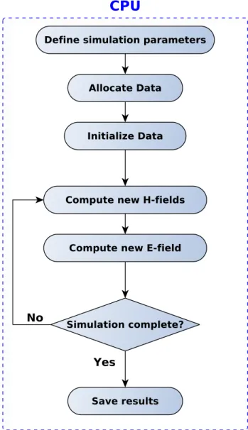
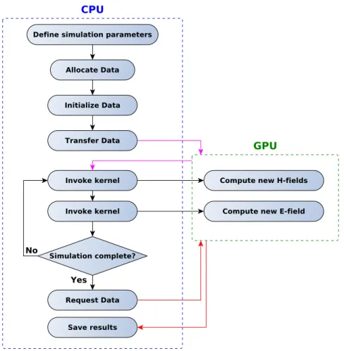
The flowchart for the FDTD method run on a CPU can be seen in Fig. 5.1. A proposed flowchart which also incorporates the GPU is shown in Fig. 5.2. The main difference being that memory transfers have been added since they are two different devices with their own embedded memory units. The computationally heavy part is now done on the GPU.

5.3.2 Design considerations

A sequential scheme could be applied and run on the GPU now as the design allows for data transfer between devices. That is, however, far from an optimal scheme for a GPU, thus some design considerations are in place.

(23)

Figure 5.1: Basic FDTD method run on CPU

Dividing the workload

A processing unit on the GPU typically have but a fraction of the computational power compared to that of a CPU. However, a GPU used for computational pur-poses can consist of several hundreds of those units, all of which can work si-multaneously. Thus in order to utilize the GPU properly, the workload needs to

(24)

Figure 5.2: Basic FDTD method run on GPU

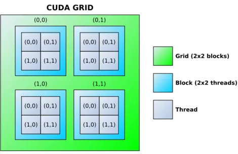
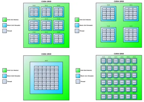
be divided evenly among those processing units. For this application it means mapping each cell to a specific thread in which the computation for that cell is specified. A CUDA thread resides in a thread block which in turn resides in a grid, both of which can have a dimensionality of 1 up to 3, depending on the GPU. The grid model can be viewed in Fig. 5.3. The next step is to dimension the grid and block so that the number of threads corresponds to the number of cells – at least. However, since the length of the dimensions in the grid and blocks can vary there are multiple solutions to this mapping scenario, all of which may perform differently. This can be seen in Fig. 5.4. In order to find suitable dimensions some testing will be needed.

(25)

Figure 5.3: CUDA thread model

Memory types

Another concern when designing applications on a GPU is that there exists differ-ent types of memory with differdiffer-ent scopes and speeds. Some examples:

• Register memory: thread specific and the fastest one

• Shared memory: block specific which makes communication between threads within a block possible

• Global memory: can be accessed by all threads in the grid, but resides off-chip and is comparatively slow

How to optimize the use of the different memory types is a complex matter and is well beyond the scope of this thesis. They should be used efficiently though.

Memory access pattern

One effective way of making better use of the global memory is to take advantage of coalesced reads. Requested memory comes in a block of bytes, whether the full

(26)

5.4. VALIDATION CHAPTER 5. MODELS & METHODS

Figure 5.4: Different grid & block sizes containing the same number of threads

block was requested or simply one byte, and are put into a cache. If other bytes which resides in that block are requested directly following that request they can be accessed through the cache(fast) instead of reloading the whole block(slow). This scheme is further explained in NVIDIA CUDA programming guide [7]. Knowing how the memory transactions work the data structures can be re-arranged in order to match that pattern. Which means seeing to that each specific property of a cell is placed next to the same property of an adjacent cell. This modification can be seen in Fig. 5.5.

5.4 Validation

The error for finite difference schemes is expected to tend to zero as its discrete operators (∆x, ∆y, ∆t) tend to zero. The rate at which the error tend to zero is known as the rate of convergence, or sometimes, order of convergence. Generally formulated as Eq. 5.1,

(27)

Figure 5.5: Array adaptations for GPU implementation

E(h) = C(hn) (5.1) where E is the error function dependent on the step size h, C a constant and n is the order of convergence. The order of convergence can be used as a measure of how accurately the FDTD method approximates the exact solution, where a higher order indicates a higher accuracy. Put simply the process will be as follows:

(28)

2. Chose a temporal step size which fulfils the CFL condition for all the spatial step sizes

3. Chose a point to observe

4. Run the different simulations and store the value of the observed point for all temporal steps

5. Calculate the order of convergence and check that it tends to 2 6. Chose a new point and go to step 4

5.4.1 Visual representation

Using subsequent heat map representations of the electromagnetic fields, the prop-agation of said fields can be visually analysed. Though not used as a way to prove the solution it can, however, give credibility to it. Moreover it can work as an early debug tool in order to find improbable behaviour. This given that the viewer possess an understanding of the physics at work. The proposed FDTD method is highly suitable for this scheme since it calculates the electric and magnetic fields for the whole problem area at all time steps.

(29)

6

Results

In this chapter the configurations and performance of the different implementa-tions will be presented. The MATLAB implementation have been replaced by an implementation in GNU Octave, moreover, another sequential implementation written in C have been added for the sake of comparison.

6.1 Test setup

OS: Ubuntu 14.04 64-bit RAM: 16 GB

CPU: Intel(R) Core(TM) i7-4770K CPU @ 3.50GHz GPU: GeForce GTX 780

NVIDIA Driver Version: 340.29

The simulations use 64-bit double-precision numbers to represent the different properties in each cell. The block size is set to (16, 16) threads and the grid size (c, c) is then set with regards to the block size and number of discrete points per dimension, n, according to Eq. 6.1

(30)

6.2. SIMULATION TIMES CHAPTER 6. RESULTS c =l n 16 m (6.1)

6.2 Simulation times

The measured times for the implementations to complete a simulation correspond-ing to a specific level of discretization can be seen in Fig. 6.1.

Figure 6.1: Simulation times for FDTD in 2D for different step sizes and imple-mentations

6.3 Computed cells per second

The efficiency of the different implementations, measured as the number of com-puted cells per second, can be seen in Fig. 6.2.

(31)

6.4. SPEEDUP COMPARISON CHAPTER 6. RESULTS

Figure 6.2: Computed cells per second for FDTD in 2D for different step sizes and implementations

6.4 Speedup comparison

The speedup factor of the implementations with respect to the Octave implemen-tation can be seen in Fig. 6.3.

6.5 Validation

The order of convergence have been calculated for a set of spatial coordinates all of which show to be 2nd-order accurate (O(h2)). The result of a specific point, (0.4, 0.3), can be seen in Fig. 6.4.

A visual representation of the electromagnetic field can be seen in Fig. 6.5, in this case depicting how much the electric field have propagated from the source, blue center, during a time period of 5 ns.

(32)

6.5. VALIDATION CHAPTER 6. RESULTS

Figure 6.3: Speedup factor for the implementations of FDTD in 2D compared to Octave for different step sizes

(33)

6.5. VALIDATION CHAPTER 6. RESULTS

(34)

7

Discussion

The MATLAB environment was not available on the test setup and as a conse-quence the original code had to be run through a different environment, in this case GNU Octave – an open-source alternative. GNU Octave is highly compatible with the MATLAB language and the code could be run as is. There is no guarantee that the program will perform the same way in the two different environments – either way these types of interpreted languages are prone to be slow when compared to compiled ones which is why an implementation in C was added.

It should be noted that if the number of cells in the simulation is not a multiple of 16 then the grid size will be oversized according to Eq. 6.1. This is still to be preferred as testing indicates that the used GPU performs better for grid sizes defined as multiples of 16, supposedly due to the inner workings of the hardware architecture. This means that if the number of cells is not a multiple of 16, there will exist dummy threads which would be mapped outside the scope of the data arrays that must be taken cared of. Moreover, it will affect performance for simulations with a low number of cells since the number of dummy threads will vary. Best performance being achieved when there are no dummy threads, i.e. the number of cells are a multiple of 16, and worst when the number of cells are a multiple of 16 plus one.

(35)

CHAPTER 7. DISCUSSION

As can be seen in Fig. 6.1, the CUDA implementation were much quicker than the other two when the number of cells increased – for the simulation with 960x960 cells, what took about one hour in Octave completed in about one minute in CUDA. It could also be seen that the computation time for the C implementation increased linearly with the increase of number of cells. This seems to be the case for the other implementations as well but only for higher levels of discretization. That can also be seen in Fig. 6.2 where both the Octave and CUDA implementations seem to converge to a constant number of computed cells per second. Further testing strengthened the sentiment, as can be seen in Fig. 7.1, where the CUDA implementation is tested for even higher levels of discretizations – this was not done for the other implementations as it would require too much time. It converges at around 1680 MCells/s, which would indicate a maximum speedup factor of around 60 and 20 times compared to the Octave and C implementations respectively. This seems to be roughly comparable with the results of Nagaoka et al. [11] who presented a speedup of 19.43 for 1024x1024 cells computed using CUDA compared to a C implementation running on a CPU.

Figure 7.1: Computed cells in millions per second for FDTD in 2D for different step sizes

(36)

CHAPTER 7. DISCUSSION

In Fig. 6.4 the value start to fluctuate after about 12 ns , this supposedly due to that the electric field at the point converge to zero. Since the method relies on the difference between discretizations, time periods with no measurable difference will yield incorrect information about the order of convergence.

(37)

8

Future work

8.1 Combining multiple parallel platforms

Combining multiple GPUs with each other in order to split up the computational burden. Since the FDTD method is highly parallel, the possibility to split up the problem domain onto separate GPUs seem viable as long as the intersections are taken care of. Combining multiple FPGAs could potentially be interesting as well, but that would suggest creating a solution for a single FPGA to begin with.

8.2 3D-FDTD

Solving the electromagnetic scattering problem in three dimensions using FDTD. The methods and models used to solve the scattering problem in two dimensions can just as well be used for three dimensions.

(38)

8.3. HARDWARE UPGRADE CHAPTER 8. FUTURE WORK

8.3 Hardware upgrade & single precision tests

Change the current GPU to one customized for numerical computations. Though they are expensive they usually have a much better performance with regards to double precision operations per time unit. It is also suggested that the implemen-tation is adapted to single precision operations and checked whether that precision is sufficient for the supposed applications.

(39)

9

Conclusion

A parallel solution to the direct scattering problem was implemented in CUDA based on FDTD in 2D. The solution was compared to sequential solutions imple-mented in C and Octave and proved to decrease the computation time in most use-cases. Analysis of the results suggested that the maximal speed-up for the parallel solution was 60 and 20 times that of the Octave and C implementations respectively. The results with regards to the validity of the 2D FDTD implementa-tion proved to be consistent with those of Monsefi et al. [8]. Suggesimplementa-tions regarding how to improve upon the existing solution have been discussed and proposed, as well as areas upon which to expand.

(40)

Bibliography

[1] L. Kun, Graphics processor unit (gpu) acceleration of time-domain finite element method (td-fem) algorithm (2009) 928–931.

URL http://ieeexplore.ieee.org/lpdocs/epic03/wrapper.htm? arnumber=5355772

[2] J. Zhang, D. Shen, Gpu-based implementation of finite element method for elasticity using cuda (2013) 1003–1008.

[3] L. Zhang, W. Yu, Improving parallel fdtd method performance using sse instructions (2011) 57–59.

[4] Y. El-Kurdi, D. Giannacopoulos, W. Gross, Hardware acceleration for finite-element electromagnetics: Efficient sparse matrix floating-point computations with fpgas, Magnetics, IEEE Transactions on 43 (4) (2007) 1525–1528. URL http://ieeexplore.ieee.org/lpdocs/epic03/wrapper.htm? arnumber=4137716

[5] L. Mattes, S. Kofuji, Overcoming the gpu memory limitation on fdtd through the use of overlapping subgrids, in: Microwave and Millimeter Wave

(41)

Tech-BIBLIOGRAPHY

nology (ICMMT), 2010 International Conference on, 2010, pp. 1536–1539. URL http://ieeexplore.ieee.org/lpdocs/epic03/wrapper.htm? arnumber=5524901

[6] M. Livesey, J. Stack, F. Costen, T. Nanri, N. Nakashima, S. Fujino, De-velopment of a cuda implementation of the 3d fdtd method, Antennas and Propagation Magazine, IEEE 54 (5) (2012) 186–195.

[7] NVIDIA, NVIDIA CUDA Programming Guide 7.0, 2015.

[8] F. Monsefi, M. Otterskog, Solution of 2d electromagnetic scattering problem by fdtd with optimal step size, based on a discrete norm analysis, 2014. URL

http://www.es.mdh.se/publications/3633-[9] G. Mur, Absorbing boundary conditions for the finite-difference approxi-mation of the time-domain electromagnetic-field equations, Electromagnetic Compatibility, IEEE Transactions on EMC-23 (4) (1981) 377–382.

[10] K. Yee, Numerical solution of initial boundary value problems involving maxwell’s equations in isotropic media, Antennas and Propagation, IEEE Transactions on 14 (3) (1966) 302–307.

[11] T. Nagaoka, S. Watanabe, Accelerating three-dimensional fdtd calculations on gpu clusters for electromagnetic field simulation, in: Engineering in Medicine and Biology Society (EMBC), 2012 Annual International Confer-ence of the IEEE, 2012, pp. 5691–5694.

Computational electromagnetic modeling in parallel by FDTD in 2D