Traffic as factor in pavement design

(1)

TRAFFIC AS FACTOR 1N PAVEMENT DESIGN

by

T Larson

RAPPORT Nr 107

(2)

STATEN S VAGINSTITUT- STOCKHOLM

The National Road Research Institute, 114 28 Stockholm, Sweden

TRAFFIC AS FACTOR IN PAVEMENT DESIGN

by

T Larson

RAPPORT Nr 107

(3)

SVI. Rapport. Nr 107.

'FOREWORD

This report is one of two prepared during the writers association with the Swedish Statens vaginstitut in the

summer of 1970. Mr Nils G Bruzelius, Director of the Institute, outlined the task in a letter of March 11, 1970 (Ref 39-70-0209)

in.which he suggested that principal attention be given " to application of the American road design criteria to the design of roads in Sweden . The work was performed under the

immediate direction of Mr Olle Andersson, Chief, Road Foundation Department.

0..

The writer had no previous knowledge of the Swedish roads or of the design methods used in that country. Therefore the two

papers are essentially briefing documents for those actually engaged in revising current pavement design procedures. During

the course of the summer, however, field trips and personnel travel provided an extensive overview of the excellent Swedish road system. Some of the opinions expressed in these papers are based on this limited type of observation.

The professional and administration staff of the Institute were

unfailingly gracious and helpful in prov1ding the many kinds of assistance a foreign traveler and worker needs. For everything

they have done and for the opportunity to work and live in

Sweden I express a very real gratitude.

T Larson

(4)

SVI. Rapport. Nr 197

Larson, T: Traffic as a factor ... Page 2

TRAFFIC AS A FACTOR IN PAVEMENT DESIGN

CONTENTS

LIST OF TABLES AND FIGURES

SUMMARY

INTRODUCTION

BACKGROUND

Effects of Traffic on Pavements

Requirements for a Mixed Traffic Index The Equivalent Wheel Load Concept

EXAMPLES OF PAVEMENT DESIGN TRAFFIC INDICES The Asphalt Institute

Great Britain Pennsylvania California

COMMENTS RELATING TO A SWEDISH TRAFFIC INDEX

REFERENCES

(5)

LIST OF TABLES

l. Cmmparison of Minimum Thickness Requirements

2. Equivalent Single Axle Load Factors

3. Typical Loadometer Data, Pt AC 41

4. Typical Loadometer Data, Pt AC 41, Page 2 5. Typical Loadometer Data, Pt D 11

6. Typical Loadometer Data, Pt D 11, Page 2

7. Calculations of Equivalency Factors Based on Shook

and Finn's Analysis of AASHO Data

8. Results of Equivalent Load Calculations, Site AC-él

9. Results of Equivalent Load Calculations, Site D-ll

10. Vehicle Classes Used in Loadometer Study

11. Comparisons of Vehicle and Axle Equivalency Factors

LIST OF FIGURES

1. Load Factors for Flexible Pavements

(6)

Larson, T: Traffic as a factor ...

Page 4

SUMMARY

The question of whether or not traffic load repetitions should be considered in pavement design, and if so by what relation-ship, is considered. From reports covering widely different experiences it is concluded that a continuum of pavement reaponse to traffic has been described. Local design practice together with traffic and environmental factors determine the sensitivity for any particular case. Comparisons between dimensions for roads of similar specification in Sweden, the UK and several states of the USA suggest that Swedish pavements might be rather insensitive to traffic loads.

A method for treating mixed traffic is required for the

development of a pavement design traffic index. The equivalent wheel load concept, with equivalency based on equal decrements

of serviceability, has been widely used for this purpose in the USA. This approach is justified through mathematical models relating pavement thickness to load applications. Such models reflect specific conditions and pavement design methods and so must be validated before any general adoption of load

equivalency factors developed elsewhere can be considered. A method for such validation based on experience in Minnesota is described.

Several traffic indexes are examined. The "standard" axle

approach used in the revised version of British Road Note 29

appears to offer convenience and an apprOpriate level of SOphistication.

Loadometer data (1966) are used to characterize the truck

traffic at two stations on the E4 road. From this very limited and out dated sample it appears that the "average" Swedish

truck is heavier than the others considered. As evidence of the instability of this parameter, even on a single road system, this average is different at the two loadometer points on the E system.

The number of standard axles calculated in the examples appears to be generally similar to that experienced on heavy duty roads elsewhere while, as noted earlier, the pavement dimensions are greater than those calculated for selected countries and states using assumed comparable conditions.

The new method for traffic and loadometer data collection proposed by Statens vaginstitut will serve the needs of a traffic index. The principal requirement for developing such an index appears to be the validation of the mathematical models relating pavement dimensions to load application in order that acceptable load equivalency factors can be specified.

(7)

TRAFFIC AS A FACTOR IN PAVEMENT DESIGN

INTRODUCTION

Several questions should be considered before undertaking the

development of a traffic index for pavement design. First there is the matter of whether or not traffic is a significant

contributor to the loss of pavement serviceability. It has been argued that if the road structure is designed to support some maximum load and to withstand climatic effects then load repetitions, per se, are relatively inconsequential. A related

question, if it is established that load repetitions are

significant, concerns Egg the traffic spectrum affects pavement serviceability. What is the nature of the relationship between pavement performance and wheel load applications?

Beyond these fundamental questions, and assuming that a traffic index for pavement design is necessary, there are practical problems. These include determining the nature of the index to be developed with respect to data availability and establish-ing techniques for extendestablish-ing its use to the entire road system.

A meaningful traffic index must accurately describe the loads to be supported by any existing or future road over its design

life. In some cases it might also be desirable to describe the

load history of existing roads.

Particularly since the AASHO road test there has been increased attention given to the matter of relating pavement dimensions to traffic. For example, the 3rd edition of Road Nete 29

(pending for publication) relates road dimensions to the total number of "standard" axle loads anticipated over the design

life. Similarly many states in the USA new follow the very

early example of California and have a traffic index in their

pavement design method.

The purpose of this paper is to consider the questions just stated in the context of the Swedish road system.using research

and development work from.UK and the USA. Following this, some

comments are offered concerning how a Swedish pavement design traffic index might be deve10ped.

BACKGROUND

Effects of Traffic on Pavements

At the AASHO road test various pavements were subjected to different but homogeneous axle loading and evaluated for present serviceability index (PSI) at frequent intervals.

(8)

Page 6

Analysis of this work (1)1) yielded curves relating decrements

in PSI to load repetitions. Furthermore, comparisons between

performance of similar pavements subjected to different loadings permitted load equivalences to be established. Similar but less detailed studies had previously been made by the State of California (2) and in connection with earlier road tests, the WASHO for example (3).

Not all road researchers, administrators and users have accepted the AASHO findings and this approach to the influence of traffic on pavements.Castiglia, et a1 (4) in a study of the AASHO road test cite the following deficiences in this work, particularly with respect to European flexible pavement practice:

a) Pavement foundations were inadequately compacted and on unusually bad soil.

b) Effects of climate were not adequately treated (they point to the WASHO test where 40 Z of the total damage occured during the second spring season after only 13 Z of the load applications). c) The entire pavement was underdimensioned to induce

rapid failure under the intense homogeneous loadings.

d) Arbitrary statistical models were used to develop factors; i.e. performance and equivalence factors, that do not have general physical significance. on using AASHO results elsewhere they summarize their position as follows:

"Concerning the tranSportation of the results obtained to conditions of structure, pavement, environment, traffic or duration that are different from those existing during the test, it should be recalled once again that very grave reservations have been made regarding the capacity of the experimental phase of the test to represent validly the situation of actual pavements in their normal condition of use.

The most judicious reply is that, regardless of the greater or lesser degree of rigour with which the HRB formulae

synthetize the data, there is no possibility of transferring these formulae to the case of different environments:"

Of course the authors of the AASHO reports did not suggest such a general use of their results. On the contrary, they specifically stated that the results could be transported

(9)

elseWhere only after extensive validating research. Guidelines for such so-called "satellite" research programs have been published by the Highway Research Board and many states in the USA have undertaken such work (5, 6).

In contrast with the AASHO test findings which emphasized traffic effects are those of Housel in Michigan. He reports that over many years of detailed observations in that state (7) climate and soil are the principal factors effecting pavement serviceability. It appears, then, that questions concerning the effects of traffic can be answered either

positively or negatively depending on the choice of references. The answer, of course, is that there exists a continuum of pavement sensitivity to traffic effects between the two extremes and the proper level can be determined only on the basis of local conditions.

The situation in Sweden with respect to such a continuum of traffic effects can only be inferred (by this writer) using background from somewhat similar regions elsewhere. Table 1 gives a comparison between thickness dimensions from several countries and states using current design procedures. Such a comparison must be used with extreme care since the parameters controlling in each design procedure can only be approximated. Minnesota has a severe climate but uses maximum spring season axle loads and as noted in Table 1 requires a pavement slightly more than one-half the thickness specified in Sweden. It might also be noted that the standard A~6 soil used in Minnesota would likely have a CBR of 3 to 6 as compared with the CBR lO estimated for class C soil (Swedish design chart).

The Pennsylvania method requires a minimum pavement thickness based on frost penetration. As shown in the table when the frost

penetration is estimated at 90 cm the required thickness is approximately 59 cm compared to 80 cm specified in the Swedish design table. It_should be noted, moreover, that this Pennsyl-vania specification has come under much criticism because it leads to over-design. The Asphalt-Institute method requires only a relatively thin full-depth asphaltic concrete layer and this is suggested as being adequate for the spring breakup period on CBerO soils. Frost heave is not directly considered in this design procedure.

From the above it might be inferred that the Swedish thickness requirement is based on frost protection and overdesigned with respect to traffic loads. If this is the case then traffic

effects on Swedish roads as now dimensioned might well be the

secondary ones from a structural vieWpoint. This is not to suggest that traffic has no influence, however. If the

(10)

SV I. Ra pp or t. Nr 10 7

Table 1. Comparison of Minimum Thickness Requirements (See Appendix I for details)

Country Soil Traffic _Thickness

(without frost) Thickness(frost minimums)

Sweden Class C UK (Pending RN 29) Minnesota »(1964 Design Table) Asphalt Institute th

(Thickness Design 8 Ed)

Pennsylvania (1968 Design Method) Moraine II FroSt gusceptible CBR 10

CBR 20

A 6 Soil CBR 10 CBR 10 > 3,000 Spring Commercial/ADT >30,000 Summer ADT 6 b 18.4x10 Standard axles

> 1,100 HCADTd

>10,000 ADT

9 Ton Spring Axle Limit

e N20 3,000 < Equiv 18,000-lb axlesg 618/1ane/day 39 46 24 45 cm cm CIT! CIR 80 45 46 24 59 cm CID cm cm CIR I «S Q U ' O Q Q l w

~ Brinck, Statens vaginstitut, Proc 94, p 17.

- Estm using 1,500 present one-way commercial traffic and a 5 2 growth rate for 20 years.

- Construction to full frost penetration depth ..estm.at 45 cm.

- This is the heaviest traffic class for this state. ,

Based on 1,500 heavy trucks per line, per day and a 20 yr.annual growth rate of 5 Z.

~ Full depth asphaltic concrete.

r Calculated using 3,000 commercial'ADT and Penna traffic factors.

- Based on 48-in (122 cm) frost penetration.

La rs on , T a I T r a f f i c as a fa ct or .. . Pa ge 8

(11)

construction is unstable or not adequately compacted rutting may occur. Also, surface polishing or wear under studded tires may be critical to the service life of the pavement. Finally,

the detailed character of Swedish truck traffic must be compared to that in the other countries represented in table 1 before any meaningful analysis of relative dimensions is possible. This matter is considered in a later section.

To sum up, the relationship between Swedish road performance and traffic follows from the Swedish design method which, in turn, reflects local conditions and practice. It is difficult, therefore, to estimate the applicabiblity of the US traffic influence factors such as equivalent wheel load and present serviceability index. It is even more difficult to assign numerical values to these terms based on foreign experiences. Nevertheless contemporary pavement design philosophy, namely that pavements should be built with the view that they will be "used up" by some volume of traffic, depends on these concepts and so their adaptation to Swedish use deserves attention.

Requirements for a Mixed Traffic Index

In the broadest sense, road traffic includes all vehicles moving over the pavement. Except on restricted residential or private industrial roads traffic includes cars, light trucks, numerous classes of heavy trucks and busses. Traffic measurements commonly identify the ADT (average daily traffic) and less commonly the percentage of trucks in the ADT. Special loadometer studies are made to identify the individual classes and weights of heavy trucks. Since loadometer data are expensive to obtain some sampling scheme is usually required for such work. This poses the further problem of aesuring that the data will be statistically reliable with respect to time, location,

class of road, and so on.

There is very general agreement that passenger cars have no significant structural effect on modern pavements. Except in unusual cases then, the mix of truck traffic should be used to deve10p a pavement design traffic index. As just noted, however, there is a mixture of trucks both with respect to size, axle configuration and loading and so some basis for dealing with this assortment must be found as the principal task in develoPing a pavement design_traffic index.

Specific data requirements for a mixed traffic index include the following:

A count by axle load increments and truck type of single, tandem and all axles at statistically selected points over the road system.

(12)

Page 10

b) Accepted equivalent axle load factors.

c) From (a) and (b), factors giving average equivalent (or "standard ) axles for truck traffic for various regions and road types.

The equivalent wheel load concept described in the next section 18 widely used as a means for systematically dealing with

mixed road traffic in the context of pavement design. The Equivalent Wheel Load Concept

The equivalence of different wheel loads or of various wheel configurations having the same load can be based on several premises;

a) that equivalent wheelloads cause similar pavements to suffer similar decrements in serviceability, b) that equivalent wheel loads cause equal deflections,

or

c) that they cause equal stress.

The equal deflection and/or equal stress bases were developed in connection with studies of landing gear configurations for heavy aircraft (8). More recently van Vuuren (9) has used this approach to study the effects on roads of very heavy vehicles, and Huang (10) has used it with elastic layered theory to study the effect of various design factors on.wheel load equivalences. The equivalence of wheel loads based on cumulative damaging effects of traffic appears to have originated in California with the so-called Brighton test track in 1940. This concept was further developed at both the Maryland and WASHO test

roads where much attention was given to comparing the effects of single versus tandem axles. The AASHO road test had as a principal objective the establishment of equivalent load factors for both flexible and rigid pavements.

Sherman (ll) explains the equivalent wheel load concept by stating that one application of a given load is equivalent in terms of potential damage to the pavement to some number of applications of a base load. Using a base load of 18,000 1b the EWL factor thus may be defined as the number of repetitions of an 18,000 lb axle load divided by the number of repetitions of some load that will cause the same amount of damage on

similar pavements. For example, a load which has an equivalence factor of 2 will, by definition, do as much damage in one

(13)

SVI° Rapport. Nr 107

axle load. Table 2 gives typical equivalent single wheel load factors.

Before looking further at the load equivalency concept it should be noted that during the AASHO Road Test Scrivner (14) proposed a theory for transforming pavement performance

equations based on homogeneous loadings to equations involving mixed traffic. He makes the following assumptions:

a) Damage accumulates over the fife of a pavement.

b) Accumulated damage can be measured by some index. c) A mathematical relationship exists between

accumulated damage and pavement design, traffic and environment.

d) Pavements with equal accumulated damage will react to a given load in the same fashion, if the pavements are of the same design and exist in the same

environment.

e) A representative sample of all loads passes each point on the pavement within a short time.

Using these assumptions Scrivner suggests equations relating total mixed traffic, pavement dimensions and performance index. The mixed load equations are derived as special cases of the single load ones and the load equivalency concept is not used.

Shook, et a1, (12) describe how the equivalent wheel load concept can reduce mixed traffic to a single traffic parameter and so accomplish what Scrivner has attempted on a more

theoretical level. The assumptions of this approach are: a) Load effects are independent of the shape of the

performance vs load applications curve. b) Load effects are independent of the order in

which various loads are applied.

c) The effect of any load can be expressed in terms of the application of some standard load.

d) Load equivalency is expressed in terms of equal decrements in performance index.

e) Pavement thickness required to maintain a given

level of performance is a function of the application of mixed loads eXpressed as equivalent loads.

(14)

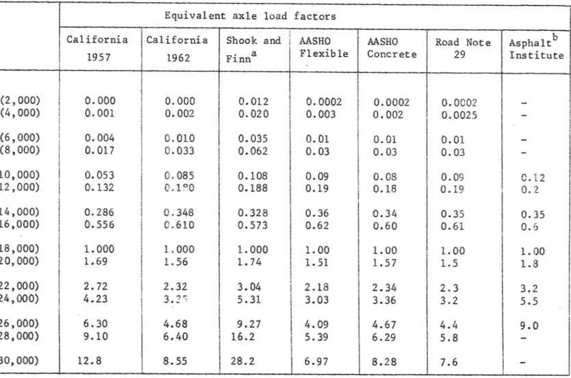
Table 2. Equivalent Single Axle Load Factors

Axle Load Equivalent axle load factors

kg (1b) _Asphaltb

Institute California California Shook and AASHO AASHO Road Note

Concrete 29 La rs on , T O O SV I. Ra pp or t. Nr 10 7 ₁₉₅₇ ₁₉₆₂ I a Finn Flexible 907.20 1,814.40 2,721.60 3,628.80 4,536.00 5,443.20

6,350.40

77,257.60 8,164.80 9,072.00 (2,000) (4,000) (6,000) (8,000) (10,000) (12,000) (14,000) (16,000) (18,000) (20,000) (22,000) 0.000 0.002 0.010 0.033 0.085 0.180 0.348 0.610 1.000 1.56 0.0002 0.003 0.00020.0025 Tr af fi c as a fa ct or .. . N v" m m 0 O N m 10,886.40 (24,000) 4.23

11,793.60 (26,000)

[6.30

4. 12,700.80 (28,000)

9.10

6

N _In m 0 \_O N 0 o 0 F 4 m o 0 4 ' 9 13,608.00 (30,000) 12.8 8.55 28.2 6.97 8.28 7.6 ~

a ~ From Shook et al, "The Use of Loadometer Data in Designing Pavements for Mixed Traffic." Highway Research

Record No. 42, 1963.

b ~ From.Fig C~1, Thickness Design, 8th Edition, The Asphalt Institute, 1969.

Pa

ge

(15)

This group of assumptions is given as purely hypothetical with no direct experimental evidence to support or deny them. They are similar to those proposed by Scrivner but more restrictive. Assumption (a) requires that load effect be independent of

the shape of the performance vs applications curve while Scrivner shows that it is9 in fact, dependent upon it. This problem is resolved when the relationship is a straight line. Assumption (b) is met if the mixed traffic notion advanced by Scrivner is satisfied, as seems likely to be the case except on special purpose roads. The remaining assumptions can be best examined using relationships suggested by Shook and Finn (13).

They suggest one general relationship between thickness and loading as

log T = a + b log Wi + c log Li (Model 1)

where: T = thickness factor

Wi = number of applications of load Li

a, b, c = factors which may or may not be functions of L or T

or T = 103 W.b L.c₁ ₁

But if thickness factor is held constant then the effect of load Li relative to an 18,000 lb load can be determined as follows:

.

lOaW.bL.C

Tl _ 1 1

T

₁₈

"

_{loE w18 18}

b c

and solving for W18 at equal thickness factor

L₁ c/b

W18 " ( 15)

then using AASHO data

(16)

Page 14

A second and the preferred model from Shook and Finn is as follows:

T = a + b log Wi + c L1 (Model 3)

where the terms are defined as before.

Solving for equal thickness factor at loads Li and 18 kip

T - a = b log Wi + c L1 = b log W18 + c 18

and

w b 10C18 .. w.b 10°13

₁₈ ₁

or

w = w.10°/b(Li "' 18)

₁₈ ₁

Again using AASHO data

w_{18 = W110}0.1405(Li a 18)

Shook and Finn have introduced a factor of safety into the preferred Model 3 so that the equivalency equation becomes

W_{18 = Wilo}0.12088(Li ~ 18)

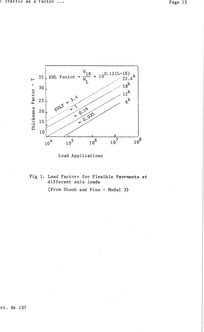
Figure 1 shows that the thickness factor applications curves of the Model 3 relationship by Shook and Finn are straight lines. Furthermores these curves are parallel. Therefore, within this model framework the equivalency factors are

independent of pavement dimensioning since T, in turn, is defined as

T = alD1 + 32D2 + a3D3

where D1, D2, D3 = thickness of surface, base and subbase reSpectively

a1, a2, a3 = material equivalency factors

The question of concern here is whether or not load equivalency factors develOped in the USA through field experience and road tests can be used elsewhere. On the basis of the previous analysis it appears that first there

(17)

z 10 k

w

w18

0.12(L~18)

35 .EWL Factor n»w _{f ).} _{2 2 a 4} L "Jr/u. 1 3 O . [du/ /uv" 8

u

IM/

»/

12 25 _

Q 3;//i://,////////// 6k

« fx» '9 //:///////

20. Q r

_M

:\ i

//f/?:/1§§ ' I 15 xx! / // 0. T h i c k n e s s Fa ct or ~ I

10 xx

//

Load Applications

Fig 1. Load Factdrs for Flexible Pavements at different axle loads

(From Shock and Finn - Model 3)

(18)

Page 16

must be confirmation or acceptance of the assumptions and the model on which the factors are based. A program for model verification might be similar to the work in Minnesota reported by Kersten and Skok (6). Basic steps include the following: a) Select research sections of relatively new roads of contemporary design to represent typical soil, load and climate conditions (use sections were a maximum of soil, construction, climate and

performance information is already available). Estimate the total load spectrum that each section

has been subjected to since it was open to traffic

and continue to record traffic and loadometer data throughout the study.

b)

Characterize the performance of the test sections using the CHLOE profilometer (15) and other devices such as wave propogation, Benkelman beam and plate bearing.

c)

Select an approach to numerical quantification of soil strength and evaluate the subgrade for each section.

d)

Use the dimensioning model and equivalent load factors deemed most apprOpriate of all available and predict performance.

e)

Modify the model and EWL factors as necessary based on experience with the test sections.

f)

Andersson (16) describes a laboratory approach for relating

Swedish soil performance to AASHO road test results. This has

the obvious advantages of lower cost and more rapid results. Castiglia, et al, (4) favoured a de~emphasis of road tests and there is currently a great emphasis on theoretical and

laboratory solutions to pavement dimensioning problems (work at the British Road Research Laboratory, Shell International, University of California, Statens vaginstitut, and Texas A and M University, for example), However, for decisions concerning a change in standard road dimensioning practice

some combination of theory and field verification will likely

be required.

EXAMPLES OF TRAFFIC INDICES FOR PAVEMENT DESIGN

Most pavement design methods include some consideration.of the effect of traffic on pavement dimensions. However, in various countries and states there are different ways of

(19)

calculating and using this traffic factor. Some typical examples will be given in the following paragraphs. The ASphalt Institute (USA)

The new thickness design manual for pavements by the Asphalt Institute contains a detailed description of the procedure for traffic analysis. In brief, a truck factor (standard axles per truck) is calculated from loadometer data9 then an initial traffic number (ITN) is determined using truck traffic counts and the previously determined truck factor. A design traffic number (DTN) is used for pavement dimensioning and reflects the projected increase in traffic over the life of the project and so is calculated using the ITN and some annual growth rate. For multilane highways the DIN is for the lane with a

concen-tration of truck traffic, normally the outmost lane. When traffic is very light (ITN 10 or less) and there is heavy auto and light truck traffic a chart is used to adjust the ITN upwards on the basis of experience.

This Asphalt Institute method uses the Shook and Finn equivalency factors in the form of curves and nomograms.

Problems of statistical reliability associated with calculating the truck factor are not discussed. The US Bureau of Public Roads guidelines for making loadometer studies are recommended for use.

Great Britain

The pending version of Road Note 29 (3rd edition) directs that

pavement design be based on the total number of "standard" axles to be carried during the design life of the project. The "standard" axle is 8,200 kg (18,000 lb) since in terms of both weight and numbers it is.the most damaging class of commercial vehicle axle on the British road system (commercial vehicles are considered to be those with an unladen weight exceeding 1,500 kg). Equivalency factors for calculating standard axles are the average of those developed at the AASHO road test for flexible and rigid pavements. Factors for calculating the number of standard axles per vehicle and per axle are given by road type and traffic volume. The total estimated number of standard axle applications over the life of the project is read from a curve after the current traffic in terms of standard axles and the traffic growth rate have been estimated. This approach includes an attractive combination of simplicity and rigor that should encourage its wide adOption and use by practicing pavement engineers.

(20)

Page 18

Pennsylvania (USA)

In the Pennsylvania pavement design method traffic is treated in terms of 18 kip daily single axle load equivalents. Axle equivalency is calculated using the AASHO flexible pavement load factors. Average truck traffic during the standard 20 year design life is estimated from the statewide loadometer and traffic counting system. Basic data for the actual route of the proposed construction project is used whenever this is

possible. The classification of trucks by truck type is

determined by means of a 24 hour survey on the route in question at a point that is representative of the entire project. Standard equivalency factors that convert truck counts to equivalent 18k axles are given for each of the major classes of trucks.

The individual truck class surveys together with the extensive traffic data available over the state make it possible to develop detailed estimates of 18 kip daily single axle load equivalents. Infact, the general precision of pavement design hardly justifies the level of refinement in this particular area.

California (USA)

The relationship between traffic and road performance in California has deveIOped from detailed observations of the road system and verification via the major road tests. In the current California pavement design procedure the following equation is given for expressing the effect of traffic.

fEWL)O.ll9 Traffic Index 6.7>

-106

The EWL (5,000 lb) applications are estimated for the design life of the project (usually 20 years). EWL constants for various classes of trucks have been developed from a

statistical sample of loaded and unloaded trucks weighed on state highways. These constants9 eXpressed as annual design EWL per vehicle per day, are given by axle group and highway class.

The pavement design equation includes the traffic index (TI) as follows

GE = 0.0032 (TI)(100 ~ R)

where GE = Gravel equivalent (a thickness index) TI = Traffic Index

(21)

It is worth noting, perhaps, that the complete performance versus thickness relationship in California was developed and only later was a traffic index identified within this equation. AASHO road test data have.been used to confirm the basic

California pavement design relationships.

COMMENTS RELATING TO A SWEDISH PAVEMENT DESIGN TRAFFIC INDEX Brinck (17) describes the Swedish loadometer studies begun in 1962. He notes that the stations for truck weighing were not chosen so as to be representative of the entire Swedish highway network and so the data must be used with discretion. By

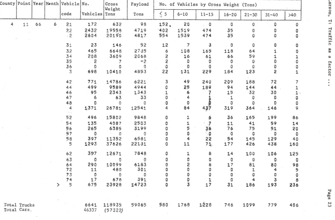
personal communication Mr. Rolf Jonsson, Statens vagverk, described how the 90 point loadometer survey is being replaced by a statistical sampling plan related to mixed traffic count and spot loadometer data. Mr. Jonsson also provided copies of data for two survey points from the extensive file collected during the time when the 90 point survey was Operated (1962-66). These are shown as tables 3, 4, 5 and 6 (two tables are used for each point. They give the 7 day results in different form). The survey points were chosen to illustrate different traffic levels on the E-system.

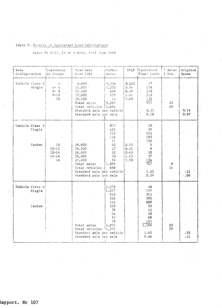
For purposes of illustration the load factor equations from Shook and Finn (also used by the Asphalt Institute) and the data provided by Jonsson were used to calculate equivalent vehicle and axle loadings for the two survey points. Calcula-tions for equivalent load factors to match the available load groups are shown in table 7.

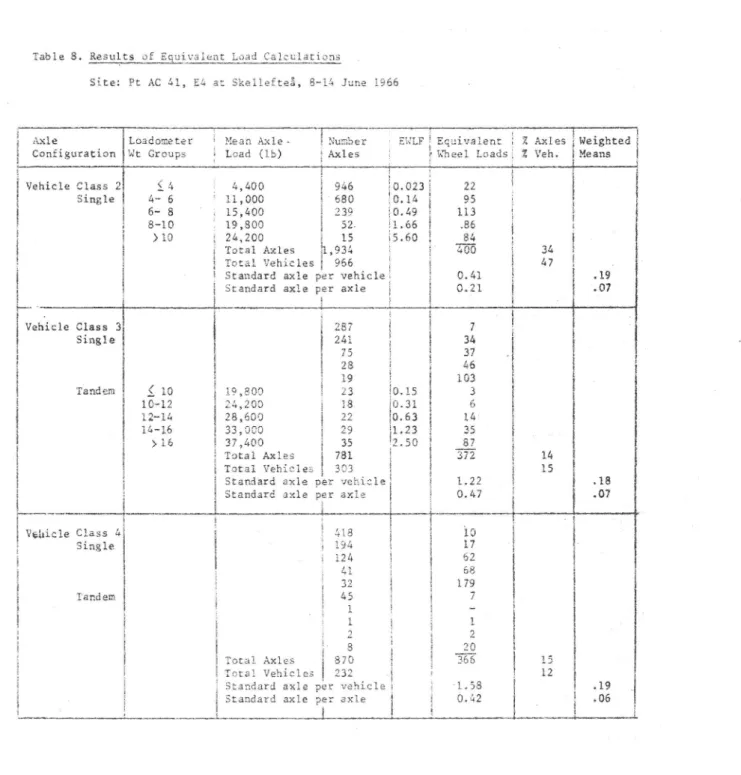
Tables 8 and 9 give "standard" axles per axle and per vehicle for each vehicle class at the two points° A weighted mean

value for these two parameters and the total number of standard axles for the seven day period is also shown. Table 10 shows the vehicle classes considered in the loadometer work.

Since the characterization of truck traffic by equivalent wheel loads has been used elsewhere, it is possible to compare

Specific traffic loadings carried by various pavement

thicknesses given in table 1. This comparison is shown in table 11. Sweden, PthC 41, shows a relatively big number of standard axles per commercial vehicle but the truck count is low at this point. Pt D ll has a slightly lower vehicle factor but the traffic count is high, thus creating an intense traffic

loading. Shook, et a1, (12) give weighted mean number of standard axles per truck for seven states in the USA. None of these is as high as the comparable value for point AC 41 in Sweden. However, the range in this value among the states in the USA

is great since each state sets the axle load weight restrictions on its highway system. In general it does appear that the

(22)

pf SE I, Ra pp . nr 10 7

.Table 32 Typigal Loadometer Data, Pt AC 41, Road E4 at Skellefteé (8 14 Jun2 1966)

ounty Pelnt Year Month Vehicle No. 6f Single Axles by axleloads No. of Tanéem Axles by axle lbads.

' d _ in tons _ in tons ~ : - _ co 8 £4 5-6, 7-8 9-10 >10 A Total $10 11 12 13-14 15~16 >16 Total J r R :

21

125

2 o

o

_

o

127

22

821

676

239

52

15 1807

2

946

680

239

52

15 1934

o

D O C . ) G O O D O C ) O D D 31 60 , 0 0 0 32 188 171 62 27 1 34 39 7o 13 1 35 0 0 I 0 o _ o o 0 0 3 287 241 75 28 1 60 0 465 0 128 23 O f) N N H 653 23 r! N N 6) o o m ' o o m o a o o o a m m m o o m o o m o o n N v-i 42 376 152 104 28 2 44 . 27 36 18 10 46 3 6 2 3 47 12 0 0 0 48 0 0 0 0 4 418 194 124 41 3 684 102 44 12 0 5 4 0 0 9 3

9

0 U 0

2

812

45

52 42 165 130, 91 92 523 14 0 4 0 0

6

0

1 0 0 0

7

H m 0 0 0 o o m o o m O W M D O Q M O H D O a m

54

12

45

15 o

74

34

56

76

59

29

21

191

56

57 .

o

0 o

58 o

o

0 o

5

130

269

174

112 .9

M N r i f f 788 104 N 385 ( 3 0 0 0 0 0 G r i t -1 0 C ) , O N N C J O Q P O C D O N O O W m I'\ m m m m 4 9 -! 1 0 62 41 152 101 60 4 63 0 O 64 44 14 72 3 6 73 6 1 74 45 2 > 5 139 175 ' 11 401 66 q 401 . 2 76 15

52 ,

551

6

c: c a c a c q c zc r o c a c n a c a c u5 h c > d ) < ) c > ¢: ) 1 1x _9'),4 ) Q' ₄₁₁

Total Axles

»

1920 .1559

h 731

300

209 4266

241

92

148 164 2329

932;

La rs on , T T r a f f i c as a fa ct ar .. .

Pa

ge

23;

(23)

$2316 6. Typicai Lea ometer Data, Pt A3 41, Page ",4. County P01nt Year Month Vehicle

a)

code No. vehicles Grqss Welght Tons Payload Tons

No. of Véhicles by Gross Weight (Tons)

<35- - 6-10 11~15 16*20 21-30 31-40 O Q A T 24 4; 66 6 21 22 2 31 32 34 35 36 3 SV I. Ra pp or t. Nr 10 7

42

44

46

47 4a

4

52

54

58

57

58

5

62 63 64 72 73 74 > £3 Total Trucks Total Cars

-a) See Table 10 with code-key.

b) This weighing Point is not included in the 90-points system

63 903 966 20 155 128 0 0 303 171 51 7 3 0 232 174 74 63 311 200 12 225 2037 19872 270 8337 8607

93 2242

2444

o

0 4779 3165 1034 215 21 0 4435 6749 2549 1456 0 0 10754 8632 0 348 219 15 169 9383 37958 23846 73 2825. 2898 12 938 1492 C 0 2442 1265 560 1387 0 1970 4657 1679 691 0 0 7027 5920 0 176 133 8 49 6286 20623 51 104 155 m ,4 " 3 0 0 0 v-l O O O N O N 0 0 0 0 0 0 0 0 0 0 0 0 0 175 12 477 489 Q l) m a r -4 °0 0 0 0 0 0 0 0 0 0 0 0 0 0 9 532 V) N m m ! 0 0 * N W '21 93 86 55 70 «a m N O N O O V o o o a o O l e a n n o un t v~o r; 458 244 0 3 0 : 0 22 41 63 23 18 43 20 15 23 0 0 9 0 1 3 0 1")

203

D O C . ) a o m o o m P O W V O C J H C ) N 64 28 O N N D D O

123

0 0 0 0 0 0 0 0 0 M O O D V 238 Tr af fi c as a fa ct or .. .A La rs on , T Pa ge 21

(24)

Table 5. Typical Loadometer.Da a, Pt D 11, Road E4 at Svérta (9~15 June 1966)

st

x

.

County Poznt Year Month VehicléINo. of Single Axles by axle loads No. of Tandem Axlés_by axle loads

code in tons in tons

{$4. 5-6 7~8 9~10 >10 Total gélo 11~12 13 14 15 16 >16 5... O (J (G ,4 R a p p o r t

4 11 66

5

21

335

7

1

9 o

344

22 2999

1243

445

128

42 4865

2 3334

1255

446

123

42 5209

O ., .9 . £3 0 0 Nr iL Q7 q -Tatal Axles 31 32 34 35 36 3 42 44 46 47 48 4 52 54 56 57 58 v '62 63 64 72 73 74 5 55,9 64 697 110 6 0 877

3.569

408 77 24 0 20?8 381 50 350 0 617 1398 201 0 537 13 0 41 792 3479 2 334 85 O O 421 717 304 $4

1977.

520 73 197

596 1386

283 477 12 36 810 4949 464 146 33

643

304

$1

151

459

925

113 397 32 552 2801 2 114 0 0 0 116 241 $5 1% 352 1?5 229 462 64 254 14 334 1 23 3 0 0 27 92 43 7 0 0 142 105 38 86 229 70 1397 208 1681 3086 999 152%? G O O D O N O O N Q 0 *0 @ V O O M N ['0 V353 96 81 178 355 260 O O Q O O Q q ? 3%a} g ! 136 110₍ 3 0 3 0 0 0 31% C 3 0 0 V } l) w. IV ) L a r i W r i D O G ( 3 9 6 3 0 0 0 m m m wa m 3 9 m m m C) !! ! H {r -3 ' 6& 1) 3 0 C ) r4 '43 ' N 2} C ) H O O V O O G O O Q O Q O O V C 3 m m $ 3 }m e m , FN-126 £89 D O C ) D U Q O O C ) N m . C ) N 499 95 594 $96 271 265 1032 714 2578 La rs on , T: Tr af fi c as a fa ct or .. . Pa ge 2 1?as

(25)

Table 6. Typical Loadometer Data, Pt D 11, Page 2 .County Point Year Manth Vehicle No. Gross

Weight Payload No. of VehiCles by Gross Weight (Tons)

Tons § 5~...- n Vehicles Tons 6~10 11-15 16 20 21~30 31-40 >40. SV I. Ra pp or t. Nr 10 7 Total Trucks Total Cars 66 58

52

63

64

72

73

74

172 2432 2604 23 465 208 2 0 698 771 499' 95 6 0 $371 496 135 265 0 397 1293 397 6641 46337 632

19558

20190

146 6648 3609 7 0 10410 14786 9589 2343 63 0 26781 15802 4087 6385 ' 0 11352 37626

12671

0 10099 480 O 678 23928

113935

(5732@

98 4719 4817 52 2755 2068 "2 0 4853 6221 4944 1343 33 0 12541 9848 2503 3199 0 6581 22131 7848 _ 0 6183 301 0 391

$4723

59065 152. 402 554 N H \ O N N O N V O D r f C J O V O G D C O O O D O O O O D 580 20 1519 1539 7 108 16 0 0 131 o wn V N 1768 «> v-c zv s4 wi m zc > ~r c r l C 3 0 d C 1 C 5 C 3 P )

. 0

474

3 165 61 0 0 229 ( 3 0 wa s N ? " V rwwi g w» i h wl c h t ¥¥ {B C i m H D < 3 v4 r \ 1-!

$225

0 35 35 0 118 66 0 O 184 209 94 15 319 36 11 76 54 177 14 17 31 766 426 100 81 186

1099

D O C ) G r i t -{C O N 129 438 106 80 193 779 G Q C J D D i n t ! ! ! 3 ' 160 125 9B 236 406 D O C ) O a t -{D C }? ! N H d O D O La rs on , T O 0 T r a f f i c as a fa ct or .. . Pa ge 23

(26)

Page 24

Table 7. Calculations of Equivalenoy Factors Based on Shook _Analysis of AASHO Data.

. - a

and_F1nm's

. k

10O.12088(L -18 )

Single axle equivaionoy factor a

L a axle loaé in Rips

9.12083(L 1sk)

Tandem a le equivalency factor a 10

1.1%

L = 2 Lt (Lt m Tandem.axle load)

gingle Agle Facgggg

b)

Load (Tons) Factor

2 0.023

7 0.49

9 1.66

11

5.60.

gandem Axle §ac§gg§

Load (Tons) Factor

9 0.15

11 0.31

13 0.63

15 1.23

17 2.50

a) Shook and Finn Thickness Design Relationships for Asphalt Pavemants", lst Ann Arbor Conference on Structural Design of ASphaltic Pavements.

(27)

Table 8. Results of Equivalent Load Calculations

Site: Pt AC 41, 10 a: Skellefte , 8~14 Junm f \C) ox 0

Axle Loadometer E Mean Axle» {Number f EHLF§ Equivalent é Z Axles Weighted

Con iguration Wt Groups § Load (lb) Axles ; g %eel Loads: Z Veh. Means

| i Vehicle Class 2. £_0 0,400 946 $0.023 22 % Single aw 5 = :1,000 680 30.14 95 g 6~ 8 ' g 15,400 239 0.49 113 8~10 ? 19,800 52. §1.66 .86 1 >10 24,200 15 $5.60 84 ' 5 Tara} Axles 1,934 2 ' 300 34 5 Total Vehicles 966 E 47 .

Standard axle per vehicle? 0.41 .19

Standard axle per axle 0.21 .07

*~.~ _ i .. Vehicle Class 3 287 _ 7 Single 241 34 ' 75 37 £8 46 V 19 103 Tandem g 10 19,800 .3 0.15 3 10 12 24,200 18 0.31 6 12*10 28,600 22 0.63 14 1$~16 33,009 29 1.23 35 >15 37,400 35 7 SO U§Z Total Axles ?81 372 14 Tatal Vehicles 303 15

Standard axle per vehicle 1 22 I .18

Stan ard axle per axle 0.47 .07

%

s 2 vehicle C1335 5+ I 5318 10 Single § 194 17 E .24 62 g 41 68 g 3: 179 38ndem g 45 7

g 1

0

-i 1 3 1 2 E 2 1 0 § 20 Total Axles 870 § 300 15 Tetal Vehicles 232 § 12

Standard axie per vahicle 5 '1.38 .19

Standard axle per 3x19 V 0.32 .06

f .

(28)

-Table 8. (Continued)

Site: Pt AC 51 ... Pa{.37 (D k)

Axle :Loadometer Mean Axle i Number EENLF :Equivalent $2 Axles Weighted

Configuration éwt Groups Load (1b) i Axles i EWheel Loads $2 Veh. Means

? ; L 2 § 1 T I Vehicle Class 5i 3 130 ; § 3 i Single 5 , 259 E 5 38 , ; ; 174 g g 86 g i 112 g i 186 z -96 g g 540 Tandem 3 ' 104 i E 16 E 27 g 8 i 42 g 27 g 58 g 71 130 3 _m;Z§ Total Axles 1,173 1,350 4 Total Vehicles 311 . 15

Standard axle per vehicle $.33 .65

Stanoard axles per axle 1.15 .23

Vehicle Class >5 139 3 Single 175 25 119 59 57 110 47 260 Tandem 59 10 46 14 83 52 73 92 136 340 Total axles 962 9 5 17 Total Vehicles 225 11

Standard axle per vehicle { 4.28 .&7

Standard axle per axle g 1.0 .17

I9:.1 axles all 213.595 = E 3?ZG 100

fetal vehicles all clas:3a : 3 2037 100

Total standard axle: a i 3453

3 2

weighted mean standard axle per vehicl; = 1.68

Heighted mean standard axle per a le : 0.60

5 k

(29)

Table 9. Re§ult9 0? Equivalent Luad Calcuiations

lte: Pt D~13 Ea at S rta, 9~15 June 2966

; 7 ~

Axle gLeadometer Msan Axle Number ENLF Equivaismt 3i Axlea weighted

Canigurazion :Kt Stumps Load (1b) Axle Wheel Loadsé-Z Veh. Means

. ;

Vehicle ClaS$ 2 &,500 3,334 0.023 ?7 g.

Singia 4~ a 11,003 1,255 0.14 :26 ;

é~ 8 15,i00 4&6 O.£9 220 g

8 10 19,300 128 1.6% 213 §

10 2%,200 £1 $.6L _§;§ g

Total axlés 5,209 21 E 25

g Totai v&h§c1es 2,604 g 30

? Standafd axle per vehicl: u 0.33 g 0.15

g Standard ax1e per axie 0.28 g 0.07

u..- E i Vehicle Class 3? 877 2 Single : 421 5§ i 335 11§ ' 116 195 2? . 150 Tan em 10 19,800 62 0.15 9 IOHIZ , 2A,200 27 0.31 8 12*14 28,600 32 0.53 20 14*16 33,000 30. 1.23 37 16 . 37,45 54 2.50 .ng Totai axles 1,889 747 9 Total vehiclas 698 11 .

Standard axle per vehicle 1.03 ; .12' Standard axle par axle 0.39 ' ' - +.04.;4 4

Vehicle Class 4 . 2,6?8 48 Single 1,07? 150 g 643 315 g 352 585 Q 142 800 Tandem g 353 53 E 39 12 % 64 ' '40 i 55 68 , ?8 19§ '

Total axles a,595 2,266 23_

* Total vehicles 1,371 20

Standard axle per vehicle 1.65 .33

Standard axle per axle 0.46 - ,' .11

-l . ;

(30)

.> -. .-~ » SV I. Ra pp or t. Nr 10 7 w. 4uu».- v..§... ._ _-»...- .w .... ..." ... .. haw. - . au. . . .... .-rv~ w'h . 0~"*g.n-l mr .. .. .». .«M u ,3 u . ,V I at I ,3 I?_. L». '9"?- km-2 '~LA)_{2 .} m.-' '_-f:_~ :7: -» bu m *5. "I. _{. ~4} _{_} :1: (1} t p . A r-...-.-v «-"13 11: « 0 ». "AA-..."...nW ...-r K v; Vr1 r in _r ., ta .i vx , a. .7 1 ,v «2 4 ' . "aI .23 "' i 5 » Lu_, _ J.J r - TC! Ir- 1' i_ i H C. JON.J .6 p -_, . a ah .r. x m 9': 5 "-1 «51* L C) n: w m a: Li! M m K" M * ~ ~ w w r-m x ("1; ~ .H u» w w\l m w in CH 3.x N c; w n .a. .., ; , x '3l. "'35 S l X v3. C} e / '3 n. I. p L) ' T I. a .3 {I 5 1. v. _{2'3 b; 0';- Ch J:~ (L i." m u;- h:-} _er 3 q r r) T) 1 :8. '1 L9 1 .14 ,.r v-... .._, . \; gm; LC)

i rm; (7 :... . iL_w«v?t"_r» (3 ~ I.-.x ..n 1;.) p4_, (A).. r v1.}_I _{~" "3}. a _{W x: A}, :J.r u"I =

{a} » it;a n; L.) l» r11, 13: . I if V) f :w» AU '3 "412* A.» {Ric} Lu 3 .) {a 1,; (3 Q) 3.x Ln 9 ;-UH N 20 I» U! :2" x? Cu 1:) Lo L}2"(h :. 7:; n S 3, 3 .1 '1. 4 Ci .5 0 LJ NJ 5 ; (I:.. ;_: ..-La rs on , T: Tr af fi c as a fa ct or .. . .. 4...»... Page 28

(31)

the standard axle basis and compared with other countries and states. The Swedish E~road traffic loadings (1966) appear to be generally comparable to those used in designing the heaviest classes of roads in the UK and USA. Pavement dimensions,

however, are in excess of those calculated for other countries and states.

As noted earlier, the development of a traffic index does, of course, require the selection of a load application versus deterioration model and from.this a calculation of load

equivalency factors. Once these matters are resolved then the "standard axle" approach as a means for treating traffic loads in pavement design appears to be the preferable one. It is very simple to use for all pavement design problems, including those associated with very heavy roads and industrial highways. The pending version of Road Note 29 gives an excellent description of this approach along with useful examples of application. It does seem doubtful that in Sweden a single standard-axles per-vehicle factor should be used over the entire country even for a particular class of highway. The calculations for two points of road E4 described in this paper show the variations that can occur between different regions of the country. However, through careful statistical treatment it can be made as reliable as pavement design methods in general. Deacon and Deem.(l8) have described some of the factors affecting axle load equivalencies

over a road system. Their work suggest how "standard" axle

factors could be developed for various classesof highways in various parts of the country through statistical treatment of the variables affecting this parameter.

Referring again to the requirements for a mixed traffic pavement design index stated earlier in this paper, it appears that the new Swedish scheme for gathering traffic and loadometer data will satisfy the first requirement of good data. Axle load equivalency factors, the second requirement, shouldbe based on validated models relating thickness to load applications and this must include extensive laboratory and field work. When these two requirements are met the existing method of treating mixed traffic, as illustrated in this paper, can be used to deveIOp an appropriate pavement design traffic index.

(32)

Larson, T: Traffic as 3 facts: ,e. Page 36

Table 10. Vehicle clagses used in loadometer study by Rolf Jonsson

E

. Percent 'Avg.

Axle Truck group "weighed" gross

group Symbol occurrenCe ¥eéght ._o

1963 1966 1966 code

1 4_ b Q W u. i » u A. f i

2 21 :3 0 {Kara 4&1 a~e<tiég : giii::e§:§3ta 2 4 4 0 4 5

22:

E:L....

₍₂ _o

(1...

_a _an

53,4

. 44,8

8,6

Sum PAY-18 .

55,8

49,4

8,2

31 C, o E; 5R3 15- {kart hjulbas) 1,3 1,3 6,7

32'

,

(3

.

a 1 6

3 g"? '6

a? o

o

00 o

8 8

7

5

34 1 599 593 18:1 p 00 . .

35" Ovriga Baaxliga kart hjulbas 0,1 0,1 5,8

36 léng hjulbas a _ «I «A

Sum.3~Axle 16,1 14,5. 15,7 {1 _9,8 _9,6 _20:6 ~ 0 0 O 0 o 05 c; o -- ._ 44 CL... .... m 3,0 4,3 20,1 4 o o 00 o 0 00 o 00 00 _

46' CL... ..

₀ _{00 oh}

{3W

₀ ₀₀ _o

1,3

0,9

25,8-47 Gvriga 4-axliga kart hjuibas 8,8 0,6 9,4

. X

48 1§21g hjulba

(w

( 5') , Ce)

Sum [P AX18 I 0 oz) Q o 5 54: M 1,3 1,5 33,1 0 oo 00 - 0 GO Gt)

'

. _.

....

.. .

G 7

3 1

24 a

56 c:

c; o 00 c3

5 3 0 oo

57 Svriga Ewaxliga kart hgulbas 0,? 0,1 §,G

58 ling hjulbas 0,5 2,6 31,5 A

Sum zAxle 11,3 13,8 31,1

{1

'

.

0 2

6

62 O

00 0 00

1 7

4 3

4:

53 Gvriga 6~axliga kart hjulbas (-) (~) {-}

64 léng hjulbas b,2 2,2 35,4

Sum swam .

1,9

6.6 38,6

72 ?~ax1iga kart hjulbaé {a} (-) (~}

7 74'

l ng hjulbas

1 (e)

9,3

42,2

Sum 7*Ax1é (~} 0,} 42,2

Grand total:

100,9

100,0

16,4

(33)

SV I. Ra pp or t. Nr 10

7 Table ll. Comparisons of Equivalency Factors and Pavement Loadings and Dimensions

a

(State) Highway 4 axle All Trucks Standard 18k Axles Frost No Frost

5 §

§ Country Type Equivalency Factor _{Average Annual} _{Typical Pavement Dimensions}

3 a L... -U m b n n M f V " .

Sweden (Pt 8-11) V E

1.03

1.44 506,000C

80 cm

-Sweden (Pt AC 41)

E

1.58

1.68 180,000C

80 cm

UK

Motorway

1.08 590,000d

45 cm

39 cm

Pennsylvania Interstate 9.64 - 225,000d 59 cm; 45 cm

Minnesota

Interstate 1.75

~

300,0008

46 cm

a, See Table l for details

b. The figure represents standard axles per vehicle while the second number of the set represents standard

axles per commercial axle

-c. Calculated from actual loadometer data

d. Estimated based on 1,500 commercial vehicles per day in design lane a. Reported by Kerston and Skok (6)

La rs on , T O 0 Tr af fi c as a fa ct or .. . P a g e 31

(34)

Larson, T: Traffic as a factor ... SVI. Rapport. Nr 107 Page 32 REFERENCES l. 2. 10. ll. 12. 13.

"The AASHO Road Test: Report 5 - Pavement Research". HRB

Special Report 61E, 1962.

F.N. Hveem and R.M. Carmony, "The Factors Underlying the

Rational Design of Pavements , HRB Proc 28, 1948.

"The WASHO Road Test; Part 2 Test Data, Analysis,

Findings." HRB Special Report 22, 1955.

Cesare Castiglia, et a1, "Study and Research on Road

Technique and the Economy of Infrastructures", International Road Transport Union, Geneva, 1968.

P.E. Irick and W.R. Hudson, "Guidelines for Satellite Studies of Pavement Performance , NCHRP Report 2A, 1964. M.S. Kersten and E.L. Skok, "Application of AASHO Road Test Results to Design of Flexible Pavements in Minnesota", HRB Record No. 291, 1969.

William S. Housel, "The Michigan Pavement Performance Study for Design Control and Serviceability, Preprint Vol. Supplement, lst Conference on Structural Design of Asphalt Pavements, 1962.

W.K. Boyd and C.R. Foster, "Design Curves for very Heavy

Multiple Wheel Assembliesz, Proc. Am. Soc. Civ. Engrs., Vol. 75, 1959.

D.J. Van Vuuren, "The ESWL Concept and its Application to Abnormally Heavy Vehicles on Roads", The Civil Engineer in South Africa, Vol. 11, No. 8, Aug. 1969.

Y.H. Huang, "Computations of Equivalent Single Wheel

Loads Using Layered Theory", HRB Record No. 291, 1969.

G.B. Sherman, "Recent Changes in the California Design Method for the Structural Design of Flexible Pavements",

California Dept. of Public Works, Sacramento, 1958.

J.F. Shook, et a1, "Use of Loadometer Data in Designing

Pavements for Mixed Traffic", HRB Record No. 42, 1963. J.F. Shook and F.N. Finn, "Thickness Design Relationships

for Aspahlt Pavements , Reprint Vol. lst Conf. on

(35)

SVI. Rapport. Nr 107 14. 15. 16. 17. 18.

F.H. Scrivner, "A Theory for Transforming AASHO Road Test

Pavement Performance Equations to Equations Involving Mixed Traffic", HRB Special Report 66, 1961.

0. Andersson, "Various Aspects on the Analysis of

Longitudinal Surface Profile by Means of the $10pe

Measuring Profilometer", Paper under preparation for

PIARC, Conf. , 1971.

O. Andersson, "Mbdification of AASHO Road Test Results

for Use with Other Soil Types", Paper under preparation

for PIARC, Conf., 1971.

C.E. Brinck, "Benefits of Increased Axle Loads", Proc. 94, Statens vaginstitut, Stockholm, 1968.

John A. Deacon and Robert C. Deen, "Equivalent Axle Loads for Pavement Design", HRB Record No. 291, 1969.

(36)

Page 34

APPENDIX I

Calculations for Thickness Requirements

Assumed Design Factors (See also notes to Table l)

§gil (except as noted in calculation)

Swedish Class C - Gravel, sand or normal moraine frost susceptible

Estimated CBR 10

Traffic (except as noted in calculation) ADT 30,000

Heavy commercial ADT 3,000 (average gross wt 40,000 lb) 5 z annual traffic increase Over 20 year life

Single axle load 11m: 10 tons (229000 1b}

Esaterseses

Maximum deflection for layered system calculation to be 1.5 mm. Road Note 29 m 3rd edition

Traffic - If present commercial traffic is 1,500 vehicles in

each direction Fig 3 gives total cumulagive number of commercial vehicles on design (slow) lane as 17x10 .

Cumulative standard axles from Table II. 6

17x10 x 1.08 = 1804x106 standard axles Subbase

Figure 6 specifies a minimum subbase of 150 mm for soils with CBR less than 30.

§urface and Base

Figure 7 Specifies a minimum of 10 cm surfacing plus 14 cm rolled aSphalt roadbase.

Total thickness 39 cm.

(37)

Asphalt Institute (Thickness design 8th edition) From Fig III°1 ITN = 2,200

From Fig III 3 Growth rate factor l.60(§?5 2

Therefore DTNZO = 2,200 x 1.60 = 39520

From Fig V l Total required thickness equals 9.5"

or 24 cm Minnesota (USA)

Assume 9 ton Spring season axle load limit and over 1,100 heavy

commercial vehicles (heaviest design class).

Total pavement thickness in inches of gravel equivalent is 31 l/Z in,

3 1/2-in surface 4 1/2*in

4 1n

bituminous base

bituminous treated base

8 -in

20

sand-gravel subbase . -in actual pavement or 51 cm

This design is for A-6 soil (CBR 2 to 3). For CBR 10 they may be reduced to 6uin or a total pavement thickness of 18~in or 46 cm.

Pennsylvania (USA)

Traffig (18 kip load applications over 20 years)

Assumed Design Lane Traffic (1,500 vehicles) Type Z Number 3 Factor Equiv. 18k

I 2 axle 37 555 .17 93 3 " 33 495 .48 238 4 " 20 300 .64 192 5 " 10 150 .64 95 Total 618 SVI. Rapport. Nr 107

(38)

222251225

From 2.14.26, Fig 3 the required structural number is 4.4. Table 1 gives minimum dimensions

surface 1 l/2-in

bituminous concrete base 8 ~in subbase 8 "in

Construction number (CN) must be greater than structural number (SN).

CN = alD1 + azD2 + a3D3

From.Table II a1 = 0.44 a2 = 0.40 a3 = 0.11

and using minimum values to check ON

ON 0.44(1.5) + 0.40(8) + 0.11(8) 4.74 (greater than SN 4.4)

Frost

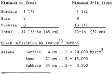
n.-Assume 3-ft penetration (90 cm). Fig 1, Section 2.14.19 requires a minimum pavement dimensions of 23~in. Therefore find

dimensions are as follows:

Minimum no frost 'Minimum 3-ft frost

Surface 1 1/2 1 1/2

Base 8 8

Subbase 8 13 1/2

Total 17 1/2 in (45 cm) 23 in (59 cm)

Check Deflection by Ivanovl) Method

20, 000 kg/cmz

Assume Surface 4 cm .. E =

Base 21 cm .. E = 15,000 Subbase 34 cm .. E = 3,500

1) USSR Report at XII World Road Congress, Rome 1964. SVI. Rapport. Nr 107

(39)

E1h1,+ Ezhz + E3h3 = 209000(4)~+15,000(21)+3,500(34)=

Average E = _{h1 + h2 + h3} ₅₉

= 8,700

9

Egeneral of the system by Koganes graph

E_{$011 _ 200}. _{__}

EL,='§2 =

E

_ave

8,700

0'023

Zr

37 1'6

where r = average radius of tire contact assumed as 18.5 cm

h = total thickness

2 thenEgeneral - 0.2 x 8,700 ~ 1,740 kg/cm

Then pavement deflection is

£l== I 1'5 p 2 2 r

(13p )

E_general

where p - contact pressure taken as 4.83 kg/cm2 poissons ratio taken as 0.3

)1

_ 1.5 x 4.83 = '

A - (1974OC1-.09)) 37 0.18 cm >0.15

Exceeds deflection criteria

(but Assumed Base "E" of 15,0001n probab1y 15w)

(40)