An ensemble learning approach based on
decision trees and probabilistic
argumentation
Istiak Ahmed
Istiak Ahmed
Spring 2020
Degree Project in Computing Science, 30 credits Supervisor: Juan Carlos Nieves Sanchez Examiner: Jerry Eriksson
This research discusses a decision support system that includes different machine learning approaches (e.g. ensemble learning, decision trees) and a symbolic reasoning approach (e.g. argumentation). The purpose of this study is to define an ensemble learning algorithm based on for-mal argumentation and decision trees. Using a decision tree algorithm as a base learning algorithm and an argumentation framework as a de-cision fusion technique of an ensemble architecture, the proposed sys-tem produces outcomes. The introduced algorithm is a hybrid ensemble learning approach based on a formal argumentation-based method. It is evaluated with sample data sets (e.g. an open-access data set and an extracted data set from ultrasound images) and it provides satisfac-tory outcomes. This study approaches the problem that is related to an ensemble learning algorithm and a formal argumentation approach. A probabilistic argumentation framework is implemented as a decision fu-sion in an ensemble learning approach. An open-access library is also developed for the user. The generic version of the library can be used in different purposes.
I would like to thank my supervisors Juan Carlos Nieves and Christer Gr¨onlund, who has contributed expertise in computer science topics and medically related topics, granting ac-cess to data used, and introducing the idea for this research, as well as providing assistance by correcting this report.
1 Introduction 1
1.1 The aim of this research 2
1.2 Organization of this research 2
2 Background 3
2.1 Ensemble Learning Algorithm (ELA) 3
2.2 Decision Tree Algorithm (DTA) 4
2.2.1 Entropy 4
2.3 Argumentation Framework 5
2.3.1 Probabilistic Argumentation Framework (PAF) 6
3 Related Works 8
3.1 Implementation of Learning Algorithm 8
3.2 Multi-Agents System 8
3.3 Data Mining Techniques 9
3.4 Argument Mining 9
3.5 Summary 10
4 Theoretical Framework 11
4.1 The formal integration between decision tree and probabilistic argumentation 11
4.2 Algorithm and analysis 12
5 Evaluation 16
5.1 An argumentation-based ensemble learning algorithm 16
5.2 Evaluation of the theoretical framework 18
5.2.1 Probability function and accuracy 23
5.2.2 Evaluation of the open-access data set 25
6.1 Functionality 32 6.2 User Manual 32 6.3 Example 34 6.4 Evaluation 36 6.4.1 Graphical Representation 36 6.5 Target User 36 7 Discussion 39
8 Conclusion and Future Work 41
1 Introduction
Machine learning approaches have a considerable contribution to develop different types of decision support systems. Learning algorithms are important for classifying data and pre-dicting outcomes based on training data [27]. A learning algorithm is an algorithm used in machine learning to assist applications to imitate the human learning process [14]. It can learn something new from a given situation. On the other hand, the symbolic reasoning is an operation of cognition that allows rules, axioms, facts, etc to generate new knowledge from existing knowledge [1]. The combined effort of the learning algorithms and symbolic reasoning can produce better outcomes [7] [18]. Whereas, it is not possible for a single approach. Many studies have been done for developing decision support systems in medi-cal science. Several artificial intelligence techniques and machine learning approaches, for instance, neural network, decision tree algorithm, multi-agents system, etc are implemented to develop a system that can easily detect dangerous diseases [15] [22] [19]. Nevertheless, there are some limitations, e.g., produce conscious outcomes, produce outcomes in case of data overlapping. The general problem statement of this research is to develop a system for the sake of resolving the limitations of previous researches that can produce conscious and satisfactory outcomes for practical usage, e.g., medical decision support systems, by implementing an ensemble architecture that includes different approaches. The research presented by Kahneman et al. (2010) introduces system 1 and system 2 [17] where system 1 produces unconscious outcomes based on training data and system 2 produces conscious outcomes through a decision making process. In this research, a learning algorithm and a probabilistic argumentation framework (PAF) are implemented as the learning approach and symbolic reasoning approach in an ensemble architecture. The learning approach and symbolic reasoning approach are implemented as system 1 and system 2 respectively. An ensemble learning algorithm (ELA) usually executes a base learning algorithm multiple times and creates a voting classifier for the resulting hypothesis [5]. ELA provides more accurate outcomes than any of its component models. It is beneficial to implement an en-semble learning approach in this specific problem. An enen-semble learning approach produces better outcomes than any single learning algorithm [24].
In this thesis, a data set of ultrasound images is used to evaluate the introduced ELA ap-proach. Moreover, decision tree algorithms (DTA) are used as the base learning algorithm of ELA that generates outcomes by classifying data set and PAF generates more accurate outcomes from the existing outcomes. DTA classifies data set from ultrasound images and generates satisfactory output with the help of the probabilistic argumentation framework. Sample data set such as an open access data set is used for evaluation of the introduced ensemble learning approach. DTA classifies data set into three different groups. Classifica-tion is a process to divide data into several groups or categories based on different decision rules. Data classification is important to categorize data set for prediction. The proposed system of combining ELA and PAF is designed to diagnosis cardiovascular diseases. Car-diovascular disease atherosclerosis is a life-threatening disease. It amasses plaque in the
carotid and coronary corridor divider, which can prompt dangerous conditions, for exam-ple, brain stroke and heart stroke [16]. It is important to develop an efficient system that can recommend the specific diagnosis to a patient by analyzing data set from ultrasound images of carotid and coronary arteries. Machine learning is useful for solving problems in the medical sector that provide promising outcomes. It is interesting to implement an argumentation approach and an ensemble learning algorithm in medical science for solving puzzles. An argumentation approach has been used for modeling aggregation and decision making [20]. The combining effort of both approaches produces accurate outcomes that are essential for medical decision support systems. Furthermore, it is an innovative idea to im-plement ELA and PAF in medical decision support systems. On the other hand, It is difficult to get accurate outcomes by implementing only machine learning approaches for detecting stroke diseases by analyzing images of the carotid and coronary arteries. The accuracy of the system depends on the machine learning model and data set.
The proposed system implements DTA for classifying the sample data set. The different approaches of DTA work like different models and they produce different outcomes. PAF generates an outcome combining the outcomes of different models. The main concern of this study is to combine the outcomes from several models of a learning algorithm (DTA) and produce feasible outputs through an argument process (PAF). The PAF works combined with DTA to generate more accurate outcomes. Both of the learning algorithm and the argu-mentation framework are crucial for this research. PAF produces more accurate output by using the outcomes from different models of DTA. The contribution of this research is to in-tegrate PAF with ELA for obtaining feasible outcomes. The different models of DTA work like a multi-agents system and the agents argue through PAF for producing an accurate and satisfactory result. A pipeline architecture is implemented to combine the learning algo-rithm and the argumentation framework. An argumentation framework works as a decision fusion in the ensemble learning approach that combines outcomes from multiple models.
1.1 The aim of this research
This study aims to introduce a probability argumentation approach as a decision fusion in an ensemble architecture. The probability argumentation approach combines outputs gen-erated from different models of an ensemble learning approach and produces final outputs. The research question is given below.
Research question: How to define an ensemble learning approach based on formal argu-mentation?
1.2 Organization of this research
The rest of the paper is designed as follows: chapter 2 presents the working procedure of ELA, DTA, and PAF; chapter 3 describes some related works in the literature; chapter 4 presents a pipeline architecture and the algorithm being used; chapter 5 analyzes the experimental results; chapter 6 discusses an open-access library, chapter 7 discusses the discussion and finally, chapter 8 presents conclusions and future work.
2 Background
This chapter discusses different approaches of ELA, DTA, and PAF. It also explains the working procedure of each approach.
2.1 Ensemble Learning Algorithm (ELA)
An ensemble learning algorithm (ELA) conducts a base learning algorithm multiple times and produces an outcome. A decision fusion technique such as a voting classifier helps to elect the optimal outcome. ELA follows a different approach such as it finds a set of hypotheses rather than finding a best hypothesis to explain the data and the hypothe-ses participate in a voting process [5]. The voting process selects an optimal hypothesis to illustrate the data. More definitely, an ensemble approach constructs a set of hypoth-esis {k1, k2, ...., kn}, picks a set of weight {w1, w2, ..., wn} and constructs a voting process
H(x) = {w1k1(x) + ... + wnkn(x)}. If H(x) ≥ 0 then the voting process will return +1
other-wise, it will return -1. The base learner components generate the hypotheses by executing a base learning algorithm which can be neural network, decision tree, or other kinds of machine learning algorithms [28]. A number of base learners can be constructed in a par-allel or sequential style. The efficiency of an ensemble method depends on the outcomes of base learners. The outcomes should be more exact and more diverse as possible. Sev-eral processes are available such as cross-validation, hold-out test, etc for calculating the accuracy of the outcomes. There are two distinct ways to design ELA. The first way is to construct the hypotheses independently that the resulting set of hypotheses is accurate and diverse. That is why each hypothesis has a low error rate for making predictions. Such an ensemble of hypotheses ensures a more accurate prediction than any of its component clas-sifiers. According to the second way, to construct the hypotheses in a coupled fashion that the weighted vote of the hypotheses provides a better structure to the data. Breiman(1996) introduces a method called Bagging (Bootstrap Aggregation) [5] [24] [2]. In this method, there is a given data set m. The different samples of data set {d1...dn} will be provided to
the different models (base learners) {m1...mn} of the base learning algorithm. The size of
each sample data set {d1...dn} is less than the source data set m. The models generates a
set of result {r1...rn}. The generated result from each model or base learner will be
con-sidered a vote. Then the voting classifier combines all of the different votes from several models and produces a final result. The result from the voting classifier is finalized based on the majority of the voting [2]. The following example explains, how does the voting classifier produce an output. For instance, five different models (m1, m2, m3, m4, m5) exist in
an ensemble approach. The models predict outcomes based on classified data and training data. The class label contains two different values, one is Y ES and the other is NO. A total of three models (m1, m3, m5) predict Y ES as outcomes and the rest of the models (m2, m4)
pro-duces Y ES as an output. The number of the vote as Y ES is greater than NO and that is why it generates Y ES as an output.
2.2 Decision Tree Algorithm (DTA)
Decision tree algorithm (DTA) is a tree-shaped diagram used to determine a course of action and each branch of the tree represents a possible decision. DTA is suitable for recommend-ing and predictrecommend-ing based on trainrecommend-ing data set. In generally, DTA constructs a trainrecommend-ing model which can use to predict class label or value of target variables. A training model consists of a set of training data and a set of decision rule and the model predicts value by learning decision rules. A training data set T S = {(x1, y1), (x2, y2), ..., (xn, yn)}, where, xi∈ X and
yi∈ Y (i = 1, ...., n). DTA starts processing from the root node for predicting a class label.
It compares the values of the root attribute with the record’s attribute. Then the algorithm follows the branch corresponding to that value and jumps to the next node. It also compares the record’s attribute values with other internal nodes of the decision tree. The process will be continued until reach the leaf node. The leaf node contains predicted class value. A deci-sion tree follows a disjunctive normal form that presents the sum of product. Every branch from the root node to the leaf node has the conjunction (product of values) class and differ-ent branches ending in the disjunction (sum) class. The greatest challenge in DTA is to find out the attribute as a root node. Different attribute selection techniques such as information gain, Gini index, and so on can be implemented to identify the root node at each level. In the proposed research entropy is implemented as an attribute selection technique.
DTA has two approaches for implementation one is decision tree classifier and another is decision tree regression [23]. In the classification approach, the target variable can be a discrete set of values. Furthermore, the tree produces a categorical solution like true or false, yes or no, 0 or 1 and in regression, the tree predicts values analyzing the values from previous states. In the regression approach, the target variable can take continuous val-ues. Algorithms like Naive Bayes, Logistic Regression, K-Means can work in classification problems. These algorithms are perfect for working with simpler data [12]. However, DTA is suitable to work in a classification problem with large and complex data sets. It is simple to understand, interpret, visualize and little effort required for data preparation. Decision Trees can deal with both numerical and the group of data [23]. The decision tree algorithm follows the greedy approach [27]. It uses a top-down recursive method for tree construc-tion. The ID3 algorithm is implemented in the proposed research. The algorithm constructs decision trees implementing a top-down greedy search approach. The tree has several deci-sion nodes and each decideci-sion node has two or more branches. It starts with the sample data set as the root node. Then it calculates the entropy of each attribute. It selects the attribute based on the highest or lowest entropy. The selected attribute splits the sample data set into smaller subsets. It is a recursive process. The algorithm always selects the attributes that never selected before. The leaf node represents a decision.
2.2.1 Entropy
Entropy is an important term in DTA. Entropy is the measurement of randomness and un-predictability in the data set. It is high in the decision or root nodes of the Decision Tree and it decreases gradually in the child nodes [23]. Entropy ensures the splitting points of a
data set. DTA picks a node with the highest information gain to construct or split a decision Tree. Entropy helps to select the right attribute or node for constructing a decision tree. The lowest entropy is calculated by the following equation (2.1).
Entropy=
e
∑
i=1
Pi(−log2Pi) (2.1)
Let Pibe a discrete random variable that takes values in the domain {P1,..., Pe}.
The overall entropy is calculated by the following equation (2.2).
OverallEntropy=
2
∑
j=1
Pj(lowestEntropy) (2.2)
The overall entropy determines the best splitting nodes.
2.3 Argumentation Framework
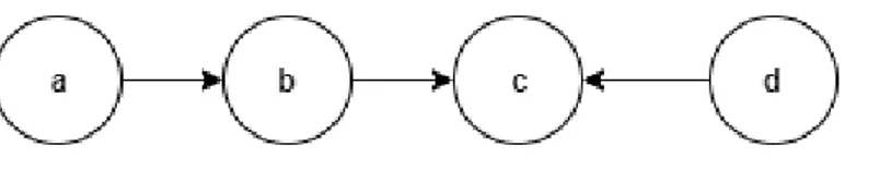
Argumentation is the process of how decisions can be decided through logical reasoning. It includes deliberation and negotiation that are important for a decision-making process. Two or more agents can participate in an argumentation process and finally, a decision can be made through an argumentation process. The strength of an argument depends on the social values and one argument attacks another. The success of an argument depends on the comparative strength of the values [1]. The argumentation framework is a pair of arguments and attacks. AF = (AR, attacks) where AR is a set of arguments and attacks is a binary relation AR [6]. For example, there are two arguments A and B. The meaning of attacks(A, B) is that A attacks on B. A set of arguments S attacks on B that means B is attacked by an argument that exists in the arguments set S. The important thing is whether a given argument should be accepted or unaccepted [6]. The example below (Fig.1) illustrates more clearly the working method of an argumentation approach. For instance, A is a set of abstract elements, and R is a set of attacks. The argumentation system S = (A, R), where, A= {a, b, c, d}, and R = {(a, b), (b, c), (d, c)} (Fig.1). A contains four arguments and R contains three attacks (a attacks b, b attacks c, d attacks c). An argument a ∈ A is acceptable with respect to E ∈ A if E defends a, that is ∀b ∈ A such that (b, a) ∈ R, ∃c ∈ E such that (c, b) ∈ R. A set of argument E is conflict-free if there is no attack between its arguments ∀a, b ∈ E, (a, b) /∈ R. An argument set E is admissible if and only if it is conflict-free and all its arguments are acceptable with respect to E. Argument labeling is a way to express the status of an argument such as where it is accepted (in), rejected (out), or undefined (undec). The following statements explain the status of an argument. ∀a ∈ A, L(a) = in if and only if ∀b ∈ A such that (b, a) ∈ R, L(b) = out. ∀a ∈ A, L(a) = out if and only if ∃b ∈ A such that (b, a) ∈ R, L(b) = in. ∀a ∈ A, L(a) = undec if and only if L(a) 6= in and L(a) 6= out. L is a set of arguments labeling that consists of a set of arguments and labeling, L= (arguments, labeling). There are different labels and the outcomes of the last example L= {(a, in), (b, out), (c, out), (d, in)}.
An argumentation approach is suitable to take an accurate decision in a complex situation. Multiple agents can argue to establish their ideas through an argumentation process. This approach provides optimal results in case of data conflicting or overlapping. That is why
Figure 1: There are four nodes a, b, c, and d define four arguments and the edges presents the attacking relation between arguments.
it is fruitful to implement an argumentation approach for generating more reliable results. In the proposed system, an argumentation approach is implemented as a decision fusion approach instead of a voting classifier.
2.3.1 Probabilistic Argumentation Framework (PAF)
Probabilistic argumentation defines different formal frameworks regarding probabilistic logic. There are different approaches of the probabilistic argumentation frameworks [8]. In the probabilistic argumentation process, qualitative aspects can be handled by an underlying logic and quantitative aspects can be captured by probabilistic measures. The underlying logic can be different rules and the probabilistic measure can be the probability, weight, or other measurements. The process can be divided into the constellations approach and the epistemic approach [9] [26]. In the constellations approach, the probabilities of arguments and attacks are considered as probabilistic assessments. The probabilistic assessments eval-uate the acceptability of arguments. In the epistemic approach, one believes more in an ar-gument rather than an arar-gument attacking it. This approach is modeling beliefs and agents. The agents are unable to change or directly add in the argumentation graph. The probabili-ties of arguments are denoting as the belief that an argument is acceptable. P is a probability function and A is an argument, P(A) ≥ 0.5 denotes that the argument is believed, P(A) ≤ 0.5 denotes that the argument is disbelieved, and P(A) = 0.5 denotes that the argument is nither believed or disbelieved [9]. The arguments in the graph that are believed to be acceptable to some degree (i.e. P(A) ≥ 0.5). Figure 2 illustrates an argumentation process where A, B, C are three arguments. The attacking relation of arguments is defined according to the rules of the admissible arguments framework. {A,C} is an admissible argument set. An argument A attacks an argument C because {A,C} is conflict-free and they satisfy the rules of the admissible argumentation framework. Whereas, {A,B} and {B,C} are not conflict free, A directly attacks B and C directly attacks B.
Figure 2: There are three nodes A, B, and C defines three arguments and the edges presents the attacking relation between arguments.
In the proposed study, two approaches of DTA namely decision tree classifiers (DTC) and decision tree regressors (DTR) work as two models component of ELA. The two different result sets from DTC and DTR act like two nodes and each node acts as an argument. A and Bare the two different sets of arguments. In admissible arguments, A does not attack itself, but A attacks B and B attacks A. Figure 3 illustrates the admissible arguments, where {A, B} is a set of arguments and they attack each other based on the probabilities of the arguments. In this scenario, Attacks is defined in a different way in the settings of ELA. The accuracy
of an argument is calculated by different probability functions that are discussed in the Evaluation chapter. The accuracy works as the probability of an argument. The probability values of arguments define attacking relations. It decides which argument will attack whom. The argument with high probability attacks the argument with less probability.
Figure 3: There are two nodes A and B defines two arguments and the edges presents the attacking relation between two arguments.
AF= (AR, Attacks) (2.3)
According to the Figure 3, AR = {A, B} and Attacks = {(A, B)}or{(B, A)}. The attacking relations depend on the probabilities of the arguments. An argument with high probability attacks the argument that holds less probability. For example P(A) = 0.8 and P(B) = 0.46 that means P(A) attacks P(B) and P(B) can defend. In this example, P(A) > 0.5 which means L(A) = in. L(A) is the labeling status of argument A. L(A) = in means A is accepted. Let’s discuss another example, where P(A) = 0.48 and P(B) = 0.76 that means P(B) attacks P(A) and P(A) can defend. In this example, P(B) > 0.5 which means L(B) = in. L(B) is the labeling status of argument B. L(B) = in means B is accepted. On the other hand, P(A) < 0.5 and L(A) = out that mean A is unaccepted.
If the probabilities of both arguments are above 0.5 then the argument with high probability will be accepted and the other one will be defeated. If the values of both arguments are similar then they will not attack each other (an extended rule that is implemented in the proposed system). The number of arguments nodes depends on the number of models of ELA. The outcomes from each model act as arguments. If the number of models is 3 then the number of arguments node will be 3 such as A, B, C. In case of more than two arguments, an argument with maximum probability attacks an argument that holds minimum probability and the accepted argument attacks an argument that holds the next maximum probability. The attacking process will be continued until the last argument in the process. For example P(A) = 0.8, P(B) = 0.46 and P(C) = 0.66. In this scenario, P(A) attacks P(B) and P(B) can defend. P(A) > 0.5 which means L(A) = in. L(A) = in means A is accepted. Then, P(A) attacks P(C) and P(A) > P(C), L(A) = in that means A is accepted. There are different labels such as in, out, and undec. The labels depend on the status (accepted, unaccepted, and undefined) of arguments. The proposed system implements modified rules of probabilistic argumentation framework in the settings of ELA for producing better outcomes.
A pipeline architecture is discussed in chapter 4 that implements the concepts of an en-semble learning architecture. In this architecture, decision tree classifiers and decision tree regressors are implemented as models and a probabilistic argumentation framework is im-plemented as a decision fusion technique.
3 Related Works
This chapter discusses previous researches that are related to ensemble architectures, learn-ing algorithms, and argumentation approaches.
3.1 Implementation of Learning Algorithm
The learning algorithm is implemented for data classification. The algorithm classifies data based on different class labels for prediction. It predicts the outcomes based on classified data and training data. The research presented by [13] explains a robust technique for diag-nosing brain diseases such as ischemic stroke, hemorrhage and hematoma and tumor from brain magnetic resonance (MR) and computerized tomography (CT) images. The system aims to help the physicians to detect different types of diseases for further treatments. It is implemented in a decision tree classifier to classify the data set. The data set is sent to the decision tree classifier and the classifier optimizes the data set for generating classification results. CT scan images of the brain are used for constructing training and testing data set. The classifier classifies data based on the training data set. The proposed system provides a better solution to the physicians to identify the actual diseases. The article provides a tangible idea to implement a decision tree algorithm for the proposed study.
The paper discusses three decision support systems and implemented machine learning ap-proaches. [3]. The first decision support system helps an individual to select a hospital. The system makes the decision to suggest the appropriate hospital to the individual based on mortality, complication, and travel distance. Machine learning and optimization techniques help the system to make an appropriate decision. The second system assists an individual by suggesting the diagnostic test based on the types of diseases. The system can accelerate the diagnostic process, decrease the overuse of medical tests, save costs, and improve the accu-racy of diagnosis. The third decision support system recommends the best lifestyle changes for an individual to minimize the risk of cardiovascular diseases (CVD). This system also uses machine learning and optimization techniques for recommendation. This research is an example of implementing different approaches of a decision tree algorithm for performing different tasks. In the proposed study, two approaches of a decision tree algorithm namely decision tree classifier (DTC) and decision tree regressor (DTR) are implemented.
3.2 Multi-Agents System
The research presented by [19] explains a multi-agents system where each agent remains in the network and represents a formal argumentation approach to take a consensus decision. A model-based architecture ensures reflective capabilities among the surrounding environ-ments and the agents. The model is more successful for the agents to achieve their goals.
The model will be updated when the observations of an agent’s surroundings indicate that the model is inaccurate. The agents can communicate with each other and share informa-tion among them. Moreover, the agents can alter their model to reflect the model aspect. The argumentation framework provides a consistent truth in case of conflicting and over-lapping situations. In the multi-agents system (MAS), each agent has a Bayesian Network as a model and all of the agents unitedly construct a consistent network. The formal ar-gumentation framework plays an important role to construct a consistent network. Several models of the agents argue through the formal argumentation framework and consequently, a consensus network is developed. Different models represent their joint model through the argumentation framework that works like a joint domain knowledge. The idea of working with multi-agents and argumentation framework is inspirational for the proposed research. In the proposed research, DTC and DTR work like multi-agents and the probabilistic argu-mentation framework (PAF) combines the outcomes from different agents and conducts an argumentation process.
3.3 Data Mining Techniques
The research introduced by [10] illustrates a decision tree-based approach for cardiovascu-lar diagnosis. Data mining helps to find out the unknown patterns of the data exploring a large data set. The data set contains heart bit rate, blood pressure, mental stress, breathing rate and so on. There are three phases namely data pre-processing, data modeling, and data post-processing are applied for data processing and pattern recognition. The decision tree algorithm creates a model that learns simple decision rules from the data features and pre-dicts outcomes. The ID3 algorithm is implemented to develop the system and the C4.5 algo-rithm ensures some improvements that enhance the performance of the ID3 algoalgo-rithm. The algorithm smartly conducts some crucial tasks such as choosing appropriate attributes, han-dling training data with missing attribute values, managing attributes with different costs, pruning the decision tree, and operating continuous attributes. The algorithm constructs a decision tree from the training data set using the concept of entropy. It follows the divide and conquers approach for tree construction. This research is an excellent example of a decision tree implementation for cardiovascular diagnosis. This article provides a mature knowledge to use data mining techniques for data preparation. Furthermore, it explains the decision tree construction process for detecting a particular disease.
3.4 Argument Mining
Argument mining research presented by [4] explains the process of extracting arguments component and the predicting relations (attack and support) between the participant argu-ments. The research is implemented neural network models for performing an argument mining approach. It mentions several neural network architectures for predicting the attack-ing or supportattack-ing relations between the arguments based on different data sets. The neural network models use a binary classification approach to classify the data sets. A neural net-work determines parent and child relation between the arguments. Four types of features namely embeddings, textual entailment, sentiment features, and syntactic features are cal-culated to define the parent and child relation. The parent and child arguments pass through
different layers and generate outputs. This research is an inspiration to work simultaneously with learning algorithms and an argumentation approach.
3.5 Summary
Several studies follow different approaches for solving classification problems. The pre-vious studies implement different approaches such as decision tree algorithms, neural net-works, arguments mining, and so on to classify data set for predicting outcomes. The data sets are pre-processed by different data mining techniques before transmitting to different approaches.
After all, the performance (e.g. accuracy and F-score) of a classification system is important and one should not neglect the fact that explainable outcomes might be of great importance for practical usage in e.g. medical decision support systems.
To the best of our knowledge, no previous study exists which uses an ensemble learning algorithm with an argumentation approach for analyzing classification problem. Although previous studies have analyzed similar assessment tasks by using classification algorithms or artificial intelligence (AI) approaches.
4 Theoretical Framework
This chapter introduces a pipeline architecture that integrates DTC, DTR, and PAF. It also introduces a formal algorithm of the proposed system.
4.1 The formal integration between decision tree and probabilistic argumen-tation
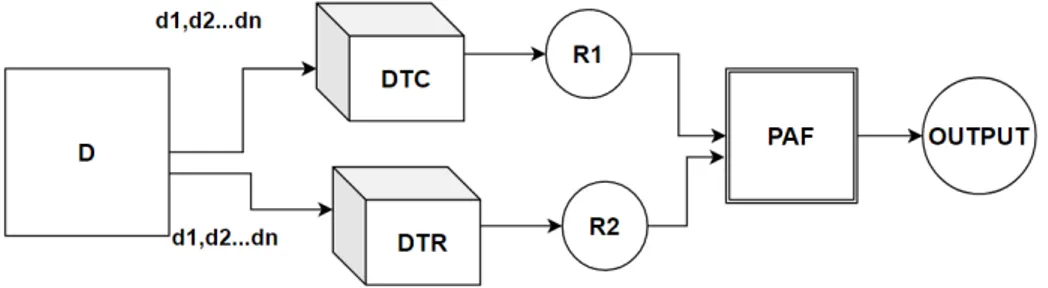
This study introduces a pipeline architecture of an ensemble learning approach. The ar-chitecture consists of different models of a learning algorithm (DTA) and a probabilistic argumentation framework. Several data mining techniques such as data fusion, data pre-processing, learning method, and decision fusion are important for pattern recognition of a data set extracted from ultrasound images. A decision tree algorithm (DTA) is implemented
Figure 4: Represent the pipeline architecture of the proposed system where D is a data source that transmits different subsets of data, e.g., d1, d2, ..., dn, to the models DTC and DTR. The size of the subsets should be less than or equal to the size of the data source. R1 and R2 contain the outputs generated by DTC and DTR. R1 and R2 send the outputs to the probabilistic argumentation framework (PAF) and PAF generates the final output.
as a learning algorithm in the proposed system. Two different approaches of DTA namely decision tree classifier (DTC) and decision tree regressor (DTR) work as two different learn-ing models. DTC and DTR classify the sample data set for prediction. Each model splits the sample data set into training and testing data set and predicts the output based on train-ing data set. The models always update their knowledge base through a learntrain-ing process for future prediction. They learn from various types of data sets and situations. The pre-dicted outputs from the models will be performed as inputs of a probabilistic argumentation framework (PAF). A classical ensemble learning algorithm implements a voting classifier as a decision fusion approach. The proposed architecture is implemented PAF instead of
a voting classifier. PAF generates outcomes through a decision-making process where the predicted outcomes from different models can argue. Furthermore, PAF helps to generate a consistent outcome in complex situations such as conflicting and overlapping information [19]. Figure 4 illustrates the pipeline architecture of the proposed system. According to Figure 4, D is a data source that contains a sample data set. The data source D divides the data set into subsets d1, d2, ..., dn. D transmits different subsets of data, e.g., d1, d2, ..., dn, to
the models namely DTC and DTR. The size of a subset is less than or equal to the size of the source data set. DTC and DTR classify the given subsets of data and predict different out-puts R1 and R2. The PAF conducts an argumentation process to produce an output. R1 and R2 are the participant arguments in the argumentation process and they attack each other. A probability function decides the attacking relation (which argument attacks to whom). If the values of both arguments are similar then they will not attack each other. The ac-cepted argument will be produced as an output. The combined effort of the models and PAF generates a reliable output.
The prototype of the proposed system is designed in Python language. Anaconda and Jupyter notebook is the integrated development environment for implementation.
4.2 Algorithm and analysis
Algorithm 1 illustrates the implemented algorithm of the proposed system. According to Algorithm 1 it analyses a sample data set S, target variables T , and attributes att. S, T , att, and estimator (number of models) are the parameter of the main function. S is a data set (e.g. test.csv) that contains numerical or categorical values. T and att are numpy array type of variables. estimator is an integer variable. le f t and right are boolean variables. S should not be empty and att should be greater than 0. “createNode” function creates nodes for all models based on the sample data set and target variables. It creates a new node by checking the availability of the left and right branches of a node. The newly created nodes will be converted into root nodes if the condition will be satisfied. “classify” function classifies the data set for the created nodes according to the different class labels. “findBestSplit” function calculates the best splitting points by calculating the entropy of different attributes. It selects an attribute as the best splitting point that holds the lowest entropy. The entropy calculation method is described in the Background chapter. Each root node has two or more child nodes. A child node can be converted into a root node by satisfying the condition of a root node. It is a recursive process. The process will be continued until finding the leaf nodes. A leaf node holds a decision. MR is an array that holds the outcomes from different models. “prediction” function predicts the outcomes of different models based on training T R and testing T S data sets. The “argumentation” function generates outcomes using MR as a set of arguments and the probabilities (P) of arguments. An argument that contains maximum probability attacks an argument that holds minimum probability. If the values of both arguments are equal then they will not attack each other. The labeling status (L) of an argument depends on the probability function. If the probability of an argument is greater than 0.5 then the labeling status will be accepted. If the probability of an argument is less than 0.5 then the labeling status will be unaccepted. If the probability of an argument is equal to 0.5 then the labeling status will be undecided. “prediction” function sends the predicted outcome sets (MR) of different models to “argumentation” function as a parameter. The values of MR argue in “argumentation” function based on probabilities and
the accepted value is considered as an output. Algorithm 2 represents the “argumentation” function. It is a simple probabilistic argumentation process. “argumentation” checks the probability of arguments. If there are more than two arguments in the process then an argument with maximum probability attacks the argument that holds the next maximum probability. The process will be continued. The experimental results of the algorithm are explained in the Evaluation chapter.
Algorithm 1 EnsembleArgumentation algorithm
procedure ENSEMBLEARGUMENTATION(S, T, att, estimator) file S = sampledataset
array T = targetvariable array att = attributes
integer estimator = numberofmodel boolean le f t = leftbranchofnode boolean right = rightbranchofnode s6= 0 & att > 0 function createNode () do node=null if le f t or right then node= root return node end if return node end function
function findBestSplit(S, att) do
maxGain← 0
splitS← null e← entropy.att for all a in S do
gain← infogain (a, e) if (gain > maxGain) then
maxGain← gain
splitS← a end if
end for end function
for all es in estimator do
if stopcondition(S, T )! = 0 then lea f = createNode () lea f.classLabel = classify () return lea f
end if
rootNode= createNode ()
rootNode.condition = findBestSplit ( S, att ) N= {n|n outcome of rootNode.condition} for all n in N do Sv= {s|rootNode.condition s ∈ S} child= Sv root← child end for end for array MR = estimator.prediction(T R, T S) array selectedarg = argumentation (MR, P) return selectedarg
Algorithm 2 Function: argumentation() function argumentation(MR, P) do ai j∈ MR
ai= max
aj= nextmax
if value(ai) = value(aj) then
No attack end if
if value(ai)! = value(aj) and P(ai) = max then
max(P(ai)) attacks min(P(a j)) end if
if value(ai)! = value(aj) and P(aj) = max then
max(P(aj)) attacks min(P(ai))
end if
if P(ai,or, j) > 0.5 then
L(ai,or, j) = in
end if
if P(ai,or, j) < 0.5 then
L(ai,or, j) = out
end if
if P(ai,or, j) = 0.5 then
L(ai,or, j) = undec
end if
return L(ai,or, j)
end function =0
5 Evaluation
The implementation of the argumentation-based ensemble learning algorithm and the ex-perimentation with different data sets such as an extracted data set from ultrasound images and an open-access data set are discussed in this chapter.
5.1 An argumentation-based ensemble learning algorithm
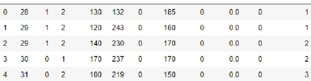
ELA is defined for implementing the proposed system that can predict the result sets based on training data sets. Two kinds of data sets were used to evaluate the proposed system. One is an open-access data set and the other is an extracted data set from ultrasound images. Figure 5 illustrates the open-access data set. The data set contains 5500 rows of data and a total of 11 attributes (Age, Sex, cp, testbps, chol, fbs, thalach, exang, oldpeak, num, and classlabel). The “classlabel” is a dependant variable and the rest of the attributes are the independent variables. The dependant variable contains three class labels such as 1, 2, and 3 which are equivalent to C1, C2, and C3. The values of the dependant variable depend on the values of the independent variables.
Figure 5: An open-access data set with a total of 11 attributes where classlabel is a de-pendant variable and the rest of the attributes are the independent variable. The dependant variable holds three class labels such as 1, 2, and 3.
Figure 6 illustrates the extracted data set from ultrasound images. The ultrasound images contain information and it is important to extract the information from ultrasound images to construct a data set. The data set contains 4900 rows of data and a total of eleven attributes. The classlabel attribute is the dependant variable that contains three values 1, 2, 3 that are equivalent to C1, C2, C3 and the rest of the attributes are the independent variables. The image segmentation approach helps to extract important information as a data set from ultrasound images. Several image filtering techniques namely Gabor, Robert, Sobel, Pre-witt, Gaussian s3, Gaussian s7, Scharr, and Median s3 applied to filter the ultrasound images for constructing the data set (Figure 6). The implemented filter techniques are used in image processing for feature extraction, stereo disparity estimation, texture analysis, and analysis
Figure 6: An extracted data set from ultrasound images with a total of 11 attributes where classlabel is a dependant variable and the rest of the attributes are the independent variable. The dependant variable holds three values such as 1, 2, and 3.
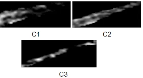
of complex oscillation. The filtering techniques extract features from ultrasound images. The values of theta, sigma, lambda, and gamma are calculated in the implementation of the Gabor filtering technique. The Robert, Sobel, Prewitt, Gaussian, Scharr, and Median are the building image filtering techniques of the scikit-image (skimage). The system can work both the open-access data set and ultrasound images. The decision tree algorithm (DTA) is used as a base learning algorithm in the ensemble learning architecture. DTA classifies the data set (sample data set or extracted data set from images) for prediction. There are three different groups of ultrasound images such as C1, C2, and C3. Figure 7 illustrates the ultrasound images based on different groups. Two approaches of DTA namely decision tree classifier (DTC) and decision tree regressor (DTR) act like two models. The models split the data set into two different data sets, one is the training data set and the other is the testing data set.
Figure 7: Ultrasound images have three different class such as C1, C2 and C3. Each class represents different information. For instance, C1, C2 and C3 represent the heath conditions of a patient such as good, bad and serious successively.
The 20% of randomly selected data from the sample data set constructs the testing data set and the rest of them construct the training data set. Entropy helps to locate the splitting point of a data set. The algorithm analyzes data from the training data set and produces outputs based on analyzed data. It learns from various situations and updates the training data set. DTC and DTR fit the training and testing data set for prediction. The models predict class labels based on the training data set. The testing data set is used as input. whereas, the training data set works as the knowledge base. Both models namely DTC and DTR take
testing data set as input and produce different result sets analyzing the input data set. The testing data set (input data set) is similar for both models. The knowledge base (training data set) helps to analyze the input data set for predicting a result set. The result set contains several class labels regarded as values. The values of two result sets can be similar or not and each value has its own accuracy. DTC and DTR send the result sets to the Probabilistic argumentation framework (PAF) for producing an output. The predicted results from both models argue in PAF. Each result act as an argument. Arguments of both models can attack each other. The accuracy function calculates the accuracy of each argument that also works as a probability in PAF. The attacking relation of arguments depends on the probabilities of arguments. An argument holding high probability attacks an argument that contains low probability. One argument is accepted through the argumentation process. On the other hand, the other is rejected. The accepted argument is regarded as a final output.
5.2 Evaluation of the theoretical framework
The results sets of the experiment are varied with different testing data sets. In this scenario, the system takes 20% of testing data sets as input and predicts outcomes. The outcomes from different models and PAF are explained below.
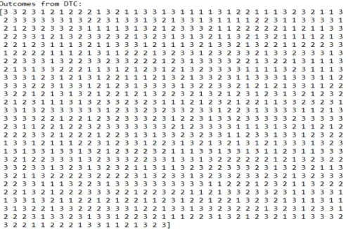
Figure 10 illustrates a predicted outcome set and graphical representation of DTC model. The outcome set (Fig.8) contains a total of 980 values and three class labels such as 1, 2, and 3. Outcomes from the outcome set of DTC act as arguments in PAF. For instance, the index positions 0, 1, 2, 3 of the outcome set contain 3, 3, 2, 3 as the outcomes, and they argue with the outcomes at index positions 0, 1, 2, 3 in the outcome set of DTR. The graphical illustration (Fig.9) depicts the graphical view of the outcome set generated from DTC. The X-axis illustrates the index positions of existing outcomes. The Y-axis illustrates the class labels (outcomes 1, 2, 3). The graph represents 980 outcomes. For example, index positions 0, 1, 2, 3, 4, 5, 6, 7, 8 present the class labels 3, 3, 2, 3, 1, 2, 1, 2, 2 respectively.
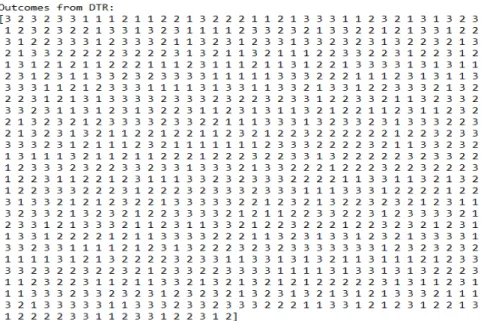
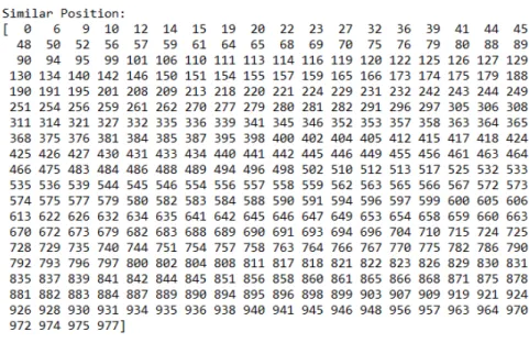
Figure 13 illustrates a predicted outcome set and graphical representation of DTR model. The outcome set (Fig.11) contains a total of 980 values and three class labels such as 1, 2, and 3. Outcomes from the outcome set of DTR also act as arguments in PAF. For instance, the index positions 0, 1, 2, 3 of the outcome set contain 3, 2, 3, 2 as the outcomes, and they argue with the outcomes at index positions 0, 1, 2, 3 in the outcome set of DTC. The graphical illustration (Fig.12) depicts the graphical view of the outcome set generated from DTR. The X-axis illustrates the index positions of existing outcomes. The Y-axis illustrates the class labels (outcomes 1, 2, 3). The graph represents 980 outcomes. For example, index positions 0, 1, 2, 3, 4, 5, 6, 7, 8 present the class labels 3, 2, 3, 2, 3, 3, 1, 1, 1 respectively. Figure 16 illustrates the similar index positions and outcomes. Figure 14 illustrates the in-dex positions of the outcome sets of DTC and DTR where they produce similar outcomes. Figure 15 represents similar outcomes according to similar index positions (Fig.14). Both outcome sets contain 346 similar outcomes according to similar index positions. Further-more, the outcomes will not attack each other. For example, at index positions 0, 6, 9, 10, 12, 14, 15, 19, 20 the outcome sets of DTC and DTR hold the outcomes 3, 1, 2, 1, 2, 1, 2, 1, 1 successively.
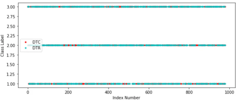
Figure 17 illustrates the graphical presentation of both result sets generated from DTC and DTR. The light blue color indicates the outcomes of DTR whereas the red color indicates
Figure 8: Represent the generated outcome set from DTC that contains 980 values. The outcome set contains three class labels such as 1, 2, 3.
Figure 9: Represent the graphical representation of the generated output set from DTC. X-axis and Y-axis illustrate the index number and the class label of the available outcome successively.
Figure 10: Represent the outcome set of DTC and graphical representation of the outcome set.
the outcomes of DTC. The X-axis and Y-axis depict the index number of existing values in the result sets and the class labels respectively. The two graphs locate some points in the same locations that imply the values of the identical location are similar. Both outcome sets contain the same class labels in the identical location and they will not attack each other. There are 346 similar values that exist in similar positions of both outcome sets. For example, index positions 0, 6, 9, 10, 12, 14, 15, 19, 20 present the class labels 3, 1, 2, 1, 2, 1, 2, 1, 1 respectively for both of the models (DTC and DTR).
Figure 18 illustrates the accepted outcome set of PAF. The outcome set contains a total of 639 values and three class labels such as 1, 2, 3. The outcome set of PAF is different from the outcome from DTC and DTR. The outcomes from two different outcome sets (DTC and DTR) participate in an argument process through PAF. They argue among themselves for finalizing outcomes (accepted outcomes). PAF produces an outcome set that contains only accepted outcomes. For example, The outcome sets of DTC and DTR hold the outcomes 3
Figure 11: Represent the generated outcome set from DTR that contains 980 values. The outcome set contains three class labels such as 1, 2, 3.
Figure 12: Represent the graphical representation of the generated output set from DTR. X-axis and Y-axis illustrate the index number and the class label of the available outcome successively.
Figure 13: Represent the outcome set of DTR and graphical representation of the outcome set.
and 2 respectively at index position 1. The outcomes 3 and 2 argue among themselves based on probability. Finally, 3 is considered as an acceptable outcome.The accepted outcome 3 locates the index position 0 in the outcome set of PAF. Figure 19 depicts the graphical view of the accepted outcome set generated from PAF. The X-axis illustrates the index positions. The Y-axis illustrates the class labels. The outcome set has three different class labels such as 1, 2, 3. The graph represents 639 outcomes. For example, index positions 0, 1, 2, 3, 4, 5, 6, 7, 8 present the class labels 3, 2, 3, 1, 2, 2, 2, 3, 1 respectively.
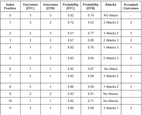
Figure 20 illustrates the attacking relations of the outcomes of different models. It represents only 12 values from the experimented outcome sets (DTC, DTR, PAF) to illustrate the attacking relations based on different probabilities and conditions. The outcome sets contain class labels such as, 1, 2, and 3. The outcomes of both models act as arguments and they attack based on probability. An outcome with a high probability attacks the outcome that contains less probability. PAF decides which argument is accepted. If the same index
Figure 14: Represent the index positions of similar outcomes from both outcome sets.
Figure 15: Represent similar outcomes based on the similar index position from both out-come sets.
Figure 16: Represent the sets of similar index positions and similar outcomes from both models (DTC and DTR).
position of both outcome sets holds similar values then they will not attack. For example, the index positions 0, 6, 9, 10 of both outcome sets hold 3, 1, 2, 1 as the similar outcomes respectively and they do not attack. At index position 1, the outcomes sets of DTC and DTR hold 3, 2 as the outcomes. The probability of outcome 3 is 0.72, whereas, it is 0.63 for outcome 2. Outcome 3 attacks outcome 2. Finally, outcome 3 is accepted through an argumentation process. The outcome sets of DTC and DTR hold the outcomes 3 and 2 respectively at index position 3. The probability of outcome 2 is 0.88, whereas, it is 0.67 for outcome 3. The outcome 2 attacks outcome 3 and 2 is regarded as the accepted outcome. In similarly, The outcome sets of DTC and DTR hold the outcomes 2 and 1 respectively at index position 7. The probability of outcome 1 is 0.94, whereas, it is 0.92 for outcome 2. The outcome 1 attacks outcome 2 and 1 is regarded as the accepted outcome. Similarly, the rest of the outcomes of DTC and DTR attack each other based on probability and PAF produces the outcome set of accepted outcomes.
Figure 17: Represent the generated output sets from DTC and DTR. Y-axis and X-axis illustrate the different class labels and the index position of the values suc-cessively. Both of the result sets have some similar values in similar index positions.
Figure 18: Represent the accepted outcome set of PAF that contains 639 values. The out-come set contains three class labels such as 1, 2, 3.
Figure 19: Represent the generated accepted output set from PAF. Y-axis and X-axis illus-trate the different class labels and the index number respectively.
5.2.1 Probability function and accuracy
This section discusses two probability equations that are implemented to calculate the prob-ability of an argument. Probability1 : (y, ¯y) = (n ÷ s) (s−n)
∑
i=0 1( ¯y= yi) (5.1)n= number of match element
s= number of sample element (a total number of element) i= index number of element
Equation 5.1 illustrates a probability equation where n, s, i define number of match element, number of sample element, and index number of element successively. The probability of result sets from different models is calculated by the probability equation.
Probability2 : p = (T P + T N)/(T P + FP + FN + T N) (5.2)
T P= true-positive T N = true-negative FP= false-positive
Figure 20: Represent the attacking relation between different arguments based on the prob-ability and shows the final accepted outcomes.
FN = false-negative
Equation 5.2 illustrates a probability equation where T P, T N, FP, FN define true-positive, true-negative, false-positive, and false-negative successively. True-positive means the actual condition is positive, but it is truly predicted as positive. Whereas, true-negative defines the actual condition is negative and it is truly predicted as negative. False-positive means the actual condition is negative, but it is falsely predicted as positive. Whereas, false-negative denotes the actual condition is positive, but it is falsely predicted as negative. The probabil-ity of result sets from different models is also calculated by the probabilprobabil-ity equation. It is a common equation for calculating the accuracy of a decision tree algorithm. Both equations are applied for calculating the accuracy of results. The accuracy of a result is regarded as the probability of an argument. The probability of arguments plays a significant role in the probabilistic argumentation framework for data mapping. In this scenario, equation 5.1 performs better than equation 5.2. The accuracy of equation 5.1 is comparably higher than equation 5.2.
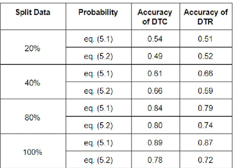
Figure 21 explains the accuracy of DTC and DTR based on the amount of splitting data and probability function. Two different probability equations (eq.(5.1) and eq.(5.2)) are applied for calculating the accuracy of different models. Using eq.(5.1) in the case of 20% split data, the accuracy of DTC is 0.54 whereas it is 0.51 for DTR. On the other hand, it is 0.49 for DTC and 0.52 for DTR by using eq.(5.2). Using eq.(5.1) in the case of 100% split data, the accuracy of DTC is 0.89 whereas it is 0.87 for DTR. In contrast, it is 0.78 for DTC and 0.72 for DTR by using eq.(5.2). The accuracy increases with the increasing amount of splitting data. Analyzing the data from Figure 21 it can be said that, the efficiency of eq.(5.1) is better than eq.(5.2) for calculating accuracy.
Figure 21: Represent the accuracy of two models namely DTR and DTC based on differ-ent probability functions (eq.(5.1) and eq.(5.2)). The accuracy varies with the amount of splitting data.
5.2.2 Evaluation of the open-access data set
This section presents the evaluation of the open-access data set. In this scenario, the system takes 20% of testing data sets as input and predicts outcomes. The outcomes from different models (DTC and DTR) and PAF are explained below.
Figure 22 illustrates a predicted outcome set of DTC model. The outcome set contains a total of 919 values and three different class labels such as 1, 2, and 3. Outcomes from the outcome set of DTC act as arguments in PAF. For instance, the index positions 0, 1, 2, 3 of the outcome set contain 2, 3, 3, 3 as the outcomes, and they argue with the outcomes at index positions 0, 1, 2, 3 in the outcome set of DTR. Figure 23 depicts the graphical view of the outcome set generated from DTC. The X-axis illustrates the index and the Y-axis illustrates the class labels. The graph represents 919 outcomes. For example, index positions 0, 1, 2, 3, 4, 5, 6, 7, 8 present the class labels 2, 3, 3, 3, 3, 3, 1, 1, 3 respectively.
Figure 22: Represent the generated outcome set from DTC that contains 919 values. The outcome set contains three class labels such as 1, 2, 3.
Figure 24 illustrates a predicted outcome set of DTR model. The outcome set contains a total of 919 values and three different class labels such as 1, 2, and 3. The outcome set of DTR is different than DTC. Outcomes from the outcome set of DTR also act as arguments in PAF. For instance, the index positions 0, 1, 2, 3 of the outcome set contain 2, 2, 1, 2 as the outcomes, and they argue with the outcomes at index positions 0, 1, 2, 3 in the outcome set of DTC. Figure 25 depicts the graphical view of the outcome set generated from DTR. The X-axis illustrates the index positions of existing values in the outcome set. The Y-axis illustrates the class labels. The outcome set contains three different class labels such as 1, 2, 3. The graph represents 919 outcomes. For example, index positions 0, 1, 2, 3, 4, 5, 6, 7, 8 present the class labels 2, 2, 1, 2, 1, 1, 2, 2, 1 respectively.
Figure 23: Represent the graphical illustration of the generated output set from DTC. Y-axis and X-Y-axis illustrate the different class labels and the index number suc-cessively.
Figure 24: Represent the generated outcome set from DTR that contains 919 values. The outcome set contains three class labels such as 1, 2, 3.
they produce similar values. Figure 27 represents similar values according to similar index positions (Fig.26). Both of the outcome sets contain 285 similar values according to similar index positions. Furthermore, the values are not attack each other. For example, at index positions 0, 11, 16, 19, 23, 24, 25, 27, 34 the outcome sets of DTC and DTR hold the outcomes 2, 1, 1, 2, 1, 3, 3, 1, 3.
Figure 28 illustrates the graphical illustration of both outcome sets generated from DTC and DTR. The light blue color indicates the result set of DTR whereas the red color indicates the result set of DTC. The X-axis and Y-axis depict the index number and the class labels respectively. The two graphs locate some points in the same locations that imply the values
Figure 25: Represent graphical illustration of the generated output set from DTR. Y-axis and X-axis illustrate the different class labels and the index number respectively.
Figure 26: Represent the index positions of similar values from both outcome sets.
Figure 27: Represent similar values based on the similar index positions of both outcome sets.
of the identical location are similar. Both outcome sets contain the same class labels in the identical location and they will not attack each other. There are 285 similar values that exist in similar positions of both outcome sets. For example, index positions 0, 11, 16, 19, 23, 24, 25, 27, 34 present the class labels 2, 1, 1, 2, 1, 3, 3, 1, 3 respectively for both models
(DTC and DTR).
Figure 28: Represent the graphical presentation of the generated output sets from DTC and DTR. Y-axis and X-axis illustrate the different class labels and the index position successively. Both of the result sets have some similar values in some points.
Figure 29 illustrates the accepted outcome set of PAF. The outcome set contains a total of 634 values. The outcome set of PAF is different from the outcome sets of DTC and DTR. The outcomes from two different outcome sets (DTC and DTR) participate in an argument process through PAF. They argue among themselves for finalizing outcomes (accepted out-comes). PAF produces an outcome set that contains only accepted outcomes. For example, The outcome sets of DTC and DTR hold the outcomes 3 and 2 respectively at index posi-tion 1. The outcomes 3 and 2 argue among themselves based on probability. Finally, 3 is considered as an acceptable outcome. The accepted outcome 3 locates the index position 0 in the outcome set of PAF. Figure 30 depicts the graphical view of the accepted outcome set generated from PAF. The X-axis illustrates the index positions. The Y-axis illustrates the class labels. The data set has three different class labels such as 1, 2, 3. The graph represents 634 outcomes. For example, index positions 0, 1, 2, 3, 4, 5, 6, 7, 8 present the class labels 3, 3, 3, 3, 3, 1, 1, 3, 1 respectively.
Figure 31 represents only 12 data from the experimented outcome sets of DTC, DTR, and PAF and presents the attacking relations and accepted outcomes. It shows where the argu-ments attack each other based on probability and different conditions. An argument with high probability attacks the argument that holds less probability. If the similar index posi-tions of both outcome sets (DTC and DTR) hold similar values then they will not attack. For example, at index positions 0, 11, both of the outcome sets hold 2,1 as outcomes and they do not attack. At index position 2, the outcomes sets of DTC and DTR hold 3, 1 as the outcomes. The probability of outcome 3 is 0.77, whereas, it is 0.57 for outcome 1. Outcome 3 attacks outcome 1. Finally, outcome 3 is accepted through an argumentation process. The outcome sets of DTC and DTR hold the outcomes 3 and 1 respectively at index position 4. The probability of outcome 1 is 0.92, whereas, it is 0.76 for outcome 3. The outcome 1 attacks outcome 3 and 1 is regarded as the accepted outcome. In similarly, The outcome sets of DTC and DTR hold the outcomes 3 and 1 respectively at index position 8. The probability of outcome 1 is 0.89, whereas, it is 0.86 for outcome 3. The outcome 1 attacks outcome 3 and 1 is regarded as the accepted outcome. Similarly, the rest of the outcomes of DTC and DTR attack each other based on probability and PAF produces the outcome set of accepted outcomes.
Figure 29: Represent the accepted outcome set of PAF that contains 634 values. The out-come set contains three class labels such as 1, 2, 3.
Figure 30: Represent the graphical illustration of the accepted output set of PAF. Y-axis and X-axis illustrate the different class labels and the index number successively.
5.2.3 Evaluation of without an argumentation framework
This section represents the evaluation of an ensemble learning algorithm without an argu-mentation framework. A classical ensemble algorithm (CELA) [21], e.g., a random forest, is evaluated with an open-access data set. The 20% of randomly selected data from the data set constructs the test data set and the rest of the data constructs the training data set. The algorithm has two models (Decision tree classifiers) and it generates a different set of outcomes. Figure 32 illustrates the final outcome set. The outcome set contains 980 values. It contains the class labels 1, 2, and 3. Figure 33 presents the graphical representation of the outcome set, where the X-axis and Y-axis represent the index position and class labels successively. The graph represents 980 outcomes. For example, index positions 0, 1, 2, 3, 4, 5, 6, 7, 8 present the class labels 3, 1, 1, 3, 1, 2, 2, 3, 3 respectively.
The produced outcome set of CELA is different from the outcome set of an ensemble learn-ing algorithm with an argumentation approach. The accuracy of CELA is less than an
ensemble learning algorithm with an argumentation approach. The accuracy of CELA is 79%, whereas the accuracy of an ensemble learning algorithm with an argumentation ap-proach is 88%. The evaluation will be extended with different data sets in future work. An argumentation approach works as a decision fusion to combining the outcomes from differ-ent models. The integration of an argumdiffer-entation approach improves the performance of an ensemble learning approach.
Figure 31: Represent the attacking relations between different arguments based on the probabilities of the arguments and shows the final accepted values.
Figure 32: Represent the outcome set of a classical ensemble learning algorithm. The outcome set contains 980 outcomes.
Figure 33: Represent the graphical representation of the outcome set of a classical ensem-ble learning algorithm, where the X-axis and Y-axis represent the index position and class labels successively.
6 Open Access Library
This chapter introduces a newly developed open-access library of the proposed system namely Basicensembleargumentation. The functionality and user manual of the library are explained in this chapter. The library is available at “pypi.org” and “github.com”. Github Link: https://github.com/Istiak1992/BasicEnsembleArgumentation.git
6.1 Functionality
The library has several methods namely Classi f iers, Regressors, Argumentation, andPlotGraph. Classi f iersmethod classifies a data set and predicts outcomes using a decision tree classifier algorithm. Regressors method classifies a data set and predicts outcomes using a decision tree regressor algorithm. Argumentation method conducts an argumentation process and generates accepted outcomes. It also represents the data set of similar values and index po-sitions. Classi f iers and Regressors methods act like two different models and they produce different sets of outcomes. Argumentation method receives the produced sets of outcomes as input parameters and pursues an argumentation process. In the argumentation process, outcomes of different models attack each other based on the probability function. If the outcomes of both models are similar, then they will not attack each other. The probability function also plays a crucial role to select the status of an argument. There are three kinds of status e.g accepted, unaccepted, and undecided. PlotGraph method generates a total of four graphs. The first graph represents the outcomes of the decision tree classifier model. The second graph represents the outcomes from the decision tree regressor model. The third graph and fourth graph illustrate the outcomes from both models and the accepted outcomes from PAF respectively. The third graph also presents the attacking relations of arguments that participate in the argument process. Furthermore, the library package contains files such as setup.txt, README.md, MANIFEST.in, LICENSE.txt,CHANGELOG.txt, requirement.txt, and ensembleArgument.py. setup.txt file contains all kinds of setup and installation require-ments. LICENSE.txt file contains the license policy provided by MIT. MANIFEST.in file helps to work with different types of files (e.g. .txt, .py). README.md file explains the user manual and requirements to use the library. CHANGELOG.txt file represents information about the release date and version of the library. requirement.txt file contains the required Python packages. ensembleArgument.py file contains the definition of all of the methods.
6.2 User Manual
The user needs to set up the environment for using the library. Python 3.5 (minimum ver-sion), pandas, numpy, matplotlib, and sklearn are the required packages for the environment. A user needs to follow the following steps to use the library.
• Set up the environment with the required packages (panda, numpy, matplotlib, and sklearn).
• Install the library package.
Command Line: pip install Basicensemblelearningargumentation (Figure 34).
Figure 34: Install the library package typing the command line in the command interpreter.
• Import packages in the python file (Figure 35).
Figure 35: Import the packages in the test python file (e.g.text.py).
• Import an additional package (Figure 36).
Figure 36: Import an additional packages in the test python file (e.g.test.py).
• Upload a data set using pandas (Figure 37).
Figure 37: Upload a data set (e.g. variableName = pd.read csv(“directory/fileName”)).
• Define the independent and dependant variables. (Figure 38).
• Call the two functions namely Classifiers and Regressors and instantiate the two func-tions into two different variables such as c1 and c2. (Figure 39).
Figure 38: Represent the independent (x) and dependant (y) variables. “class label” is the last column name of the data set that contains class labels.
Figure 39: Assign the outcomes of two models into two different variables e.g. c1, c2.
• Call the Argumentation function with the required parameters (e.g.c1, c2). Instantiate the function in a variable (e.g. c3) (Figure 40).
Figure 40: Represent how to call the Argumentation function with the required parameters and instantiate in a variable.
• Call the PlotGraph function with the required parameters (e.g.c1, c2, c3) (Figure 41).
Figure 41: Represent how to call the PlotGraph function with the required parameters.
• Call the show() function to represent the graphical views (Figure 42).
Figure 42: Represent how to call the show() function to represent the graphical views.
6.3 Example
The following example (Figure 43) helps the user about using the library. To use the library user should install the required packages (section User Manual). The user should create a
python file e.g. test.py and import all of the required packages in the python file (test.py). In the next step, the user should upload a data set (Figure 37) by using pandas and define the dependant and independent variables. Call two building functions namely Classifiers and Regressors with the required parameters. Then the user should call Argumentation and PlotGraph functions with the required parameters to generate reliable outcomes and graphical representation of the outcomes successively. The user should call the show() function for the sake of representing the graphical views. The outcomes of Classifiers and Regressors functions should be placed as parameters in the Argumentation function. Example 1 (Fig.43) explains: how to implement the library in a python file. An open access data set (Fig.44) is used for the example.
Figure 43: The figure represents an example using the library.