Developing a weighting set based on monetary damage estimates: Method and case studies

(1)

Developing a weighting set based on monetary damage

estimates. Method and case studies

Sofia Ahlroth

Environmental strategies research – fms, Department of Urban studies, Royal Institute of Technology, Stockholm

Version 1.0, March 2009

Environmental strategies research– fms Department of Urban studies Royal Institute of Technology

100 44 Stockholm www.infra.kth.se/fms

(2)

Title:

Developing a weighting set based on monetary damage estimates. Method and case studies Author:

Sofia Ahlroth ISSN

TRITA-INFRA-FMS 2009:1, version 1.0 March 2009 Printed in Sweden by US AB, Stockholm, 2009

(3)

Preface

This report has been produced within the project “Common techniques for environmental systems analysis tools” (Gemensamma metoder för miljösystemanalystiska verktyg, MEMIV). The project is a cooperation between researchers from the Department of

Environmental strategies research – fms at the Royal Institute of Economic Research (KTH), the Department of Environmental Economics at the University of Gothenburg, Energy Systems Technology at Chalmers University of Technology, Environmental Technique and Management at Linköping University, Environmental Statistics at Statistics Sweden and Stockholm Environment Institute. The project is financed by The Foundation for Strategic Environmental Research – Mistra. The aim of the project is to develop and test techniques that may be common to several environmental systems analysis tools. In this report, a weighting set proposed for use in several systems analysis tools is developed.

(4)

Summary

In environmental systems analysis tools such as cost-benefit analysis (CBA) and life-cycle assessments (LCA), generic values for impacts on the environment and human health are frequently used. There are several sets of generic values, which are based on different valuation methods, e.g. willingness-to-pay, abatement costs, taxes or non-monetary

assessments. This study attempts to derive a consistent set of damage-based values based on estimation of willingness to pay (WTP) to avoid damages. Where possible we compile

existing damage cost estimates from different sources. Currently, there are no generic damage costs available for eutrophication and acidification. We derive damage values for eutrophying and acidifying substances using WTP estimates from available valuation studies. For

eutrophication, we derive benefit transfer functions for eutrophication that allows calculation of site-specific values. We compare the derived ecosystem damage values to existing

estimates of the cost for reducing nitrogen and phosphorus emissions to water. The analysis indicates that many abatement measures for nitrogen have a positive net benefit while most measures to reduce phosphorus cost more than the benefit achieved when estimated on a general level and should, instead, be assessed on a case-specific level. Moreover, a

comparison of the existing environmental taxes on nitrogen, nitrogen oxides and phosphorus in Sweden show that the current tax rates do not reflect the externalities from these pollutants. Subsequently, we construct a weighting set by combining the derived values with existing generic damage values for human toxicity, photochemical oxidants and global warming. The weighting set - labelled Ecovalue09 - is applied to three case studies and the outcome is compared to the results using other weighting sets.

(5)

1. Introduction

Impact assessments rely on valuation of environmental impacts in order to facilitate comparison of total impacts from different projects and products. These valuations can be expressed in terms of monetary values or non-monetary weights. In cost-benefit analysis (CBA), the aim is to monetise all costs and benefits from the analysed project. For example, impacts on the environment, time use and health are often monetised, making them

comparable to the monetary costs and revenues of the project. In other systems analysis tools, such as Life Cycle Analysis (LCA), Environmental Management Systems (EMS), Life Cycle Costing (LCC) and Strategic Environmental Assessment (SEA), valuation is used to assess the total impact on the environment from e.g. a product or a project, and to compare this with the impact from alternative projects or similar products (Finnveden and Moberg, 2005; Ness et al., 2007).

In the environmental systems analysis tools mentioned above, sets of generic values for different substances and impacts are frequently used. In Sweden, values for pollutants from transport are calculated regularly at the behest of the government in the so-called ASEK (Arbetsgruppen för SamhällsEkonomiska Konsekvensanalyser) projects (SIKA, 2004). These generic values are routinely used in CBAs of infrastructure planning in Sweden, a practice that has parallels in many other countries (Navrud, 2000). On the EU level, generic values for pollutants from energy generation and transport have been calculated within the ExternE program and related projects (www.externe.info, www.methodex.org). Examples of other sets of generic values, both monetary and non-monetary, include Ecotax02 (Finnveden et al., 2006), Eco-indicator 99 (Goedkoop and Spriensmaa, 2000), EPS2000 (Steen 1999) and the Ecoscarcity method (Ahbe et al., 1990). The generic values for ecosystem effects in these weighting sets are based on abatement costs (ASEK, ExternE), environmental taxes

(Ecotax02) or damage assessments/expert judgments (Ecoindicator, EPS). The aim with the weighting set derived in this paper is to form a consistent weighting set that is useful in different environmental systems analysis tools such as LCA and CBA. To be useful in such tools, the values derived should estimate the environmental change in monetary terms and capture as much of the impacts from the pollutants as possible.

(8)

To be suitable for use as generic values in cost-benefit analyses, the values should preferably reflect welfare loss connected to a lower environmental quality. For many goods and services, market prices may be a good indicator of their marginal social value, unless some market imperfection is present i.e., imperfect competition, government intervention in the market or absence of a market (Hanley and Spash, 1993). Environmental goods and services, such as clean air and swimmable water, typically do not have a market value. Several methods are available to try to determine the value of such goods. For example, one could estimate the cost to reach a certain target that society has decided upon, where the cost represents an implicit value of reducing the damage. Another method is to interpret an environmental tax as the value society attaches to an environmental improvement.

Another approach is to capture the welfare loss to individuals due to a lower environmental quality. There are a number of methods available for this approach. For example, one can use available information from related markets (so-called revealed preference methods) or by constructing hypothetical markets where people are asked to make hypothetical choices (so-called stated preference methods). Examples of the former are the travel cost method (TCM) and hedonic pricing, and the latter include methods such as contingent valuation (CV) and choice experiments. Stated preference methods are more inclusive than revealed preference methods - they can capture both use and non-use values - whereas revealed preference methods typically capture the value for a certain group of people, such as tourists or real-estate owners. However, the advantage with revealed preference approach is that it is based on real choices; in contrast stated preference methods are based on a hypothetical setting, which can give rise to several types of biases (see e.g. Mitchell and Carson (1989) for a discussion). Since the early nineties, when the NOAA panel on contingent valuation made recommendations for the use of contingent valuation (Arrow et al. 1993), these valuation methods have been further developed and applied in various policy situations (e.g. Navrud and Pruckner 1997, Pearce 2007, Methodex 2007a).

For our weighting set, we need to have a broad approach that can be used for many different types of impacts and pollutants. Thus, we have chosen to use welfare-based estimates derived from stated preference studies for non-market assets. This method is not only the most encompassing, but the availability of many valuation studies based on this method makes our

(9)

task easier. Further, we will rely on market prices when possible (i.e., in cases of market assets)

The ExternE projects (ExternE, Methodex, Espreme) have derived generic values for health effects and different pollutants, as well as effects from tropospheric ozone on crops and materials. Several studies estimate the cost of climate change (see Tol 2008). However, there are currently no generic damage values for the ecosystem effects from eutrophying and acidifying pollutants. Dose-response functions for effects on ecosystems are not as well developed as exposure-response functions for health effects. Also, ecosystems and their sensitivity to pollution differ between countries. In contrast, the human body reacts much the same to exposure to pollutants regardless of where a person lives. On the other hand, attitudes toward health risks differ greatly between countries, just as attitudes toward changes in ecosystem quality (Ready et al., 2004). However, it is possible to value end-points such as changes in ecosystem services. While the effect of different substances varies in different geographic areas, the environmental amenities themselves are similar. Here, we attempt to use a welfare-based approach to calculate generic damage values for the ecosystem impacts arising from nitrogen, sulphur and phosphorus in Sweden. The values are derived using information gathered from valuation studies estimating willingness to pay (WTP).

The report is divided into two parts. In the first part, we describe the derivation of generic values for eutrophication and acidification. Section 2 describes the methods used for

transferring WTP values, aggregating the results and calculating generic values per pollutant. Results are presented in section 3, and uncertainties are discussed in section 4. We compare our values with other generic ecosystem values for Sweden in section 5. In section 6, we compare our damage values with (1) the environmental taxes levied on these pollutants in Sweden and (2) the cost estimates of reducing nitrogen and phosphorus emissions to water.

In the second part we describe the construction of the weighting set. In section 7, the derived ecosystem damage values are combined with existing damage values for other endpoints (health effects, climate change and photochemical oxidation) as well as values for resource depletion, to form a weighting set. This weighting set is then applied to three LCA case studies in section 8, and the outcome is compared with the results when using other weighting sets. The method and results are discussed in the concluding section.

(10)

Part 1. Deriving generic values for eutrophying and acidifying

pollutants

In Part I we will derive generic values for the impacts of eutrophication and acidification on Swedish ecosystems which will be used in conjunction with other generic values reflecting damage costs in the weighting set derived in Part II. The valuation is done in three steps. First, we survey available valuations studies and select a benefit transfer method. An empirical background to the ecosystem impacts is also given. Second, we apply the chosen method and compute total values for reducing eutrophication and acidification. Third, we calculate generic values per unit of pollutant. We then compare the derived values to other generic values, as well as to tax rates and avoidance costs.

2. Valuation method

2.1 Valuation of damages

To find suitable data, we conduct a survey of valuation studies using the EVRI database (www.evri.ca), the Swedish Value BaseSWE (Sundberg and Söderqvist, 2004) and the Nordic database NEVD (Navrud et al., 2007). We complement these databases with a literature search, including both scientific journals and reports from different agencies. Due to variations in the availability of data we used different methods for valuing the various impacts. The ambition was primarily to use Swedish studies in order to capture Swedish preferences for the environment and avoid the ambiguities with transfers between countries apparent in many benefit transfer studies (e.g. Loomis, 1992; Barton, 1999; Ready et al., 2004). When this was not possible, we relied on studies from countries with a similar natural environment and economic structure to Sweden.

For reducing eutrophication levels in the entire Baltic Sea, we rely on national estimates for the value of the required quality improvement. The valuation studies for eutrophication of freshwater and coastal waters, however, generally cover a confined area such as a lake or a bay. Therefore, we require a method for extrapolating the local values to the national level in a consistent manner.

To aggregate these values we require a benefit transfer procedure, i.e. a method to transfer values estimated for one site to other sites. For this purpose, we used a method called

(11)

structural benefit transfer. A criterion when choosing a transfer method is that its application should be easy for practitioners and that it rely only on readily available data. The structural benefit transfer method is attractive in that it provides a framework based on economic theory, producing theoretically consistent estimates. Double-counting risks are also eliminated. The method is based on a theoretical framework where the utility function is calibrated from available data and the functional forms are based on theory rather than empirical estimation (much like in Computable General Equilibrium, CGE, modelling). This approach has both advantages and disadvantages. From a practical point of view, it is an advantage that the required data can be found without extensive data-mining or by performing special surveys (i.e., the high cost of data collection is the main argument for relying on benefit transfer instead of performing new valuation studies). A disadvantage with this theoretical approach is that the utility function is not based on empirical observations, but relies instead on theoretical assumptions about people’s preferences.

Another attractive quality of the method is its ability to account for both the level of quality and the size of the quality change. Further, it includes results from both travel cost (TC) and contingent valuation (CV) studies. The coastal areas along Sweden vary with regard to eutrophication levels. Due to different characteristics (e.g. salinity), the reference values of sight depth (visibility) and nutrient levels also differ. This implies that the required

environmental change to reach a given water quality will vary from area to area. When making transfers to coastal areas it is desirable to adjust for these types of differences (e.g., in the level and required quality improvement). There were two types of valuation studies available that estimated the value of improved water quality at coastal areas in Sweden: TC studies and CV studies. In the TC studies on water quality from Sweden, the estimated functions included sight depth as a variable (the indicator used for water quality). In the CV studies, the valuation functions did not include quality levels or quality change. This

information is, however, provided in the TC studies, which argues for a method that can integrate these TC and CV studies. As with any other benefit transfer procedure, it is

important to take into account both similarity of sites and the quality changes when doing the transfer. In the following, we will describe the logic behind the method. The description draws heavily on Smith et al. 2000, where a more detailed description can be found.

(12)

The basic idea is to calibrate a utility function using the measures estimated in valuation studies. TC studies, hedonic pricing (HP) studies and CV studies all give estimates of different economic measures that can be linked to a common utility function. Here, we will deal with measures from TC and CV studies.

We rely on a utility function from the frequently-used Cobb-Douglas form. To capture the recreational values we use a cross-product repackaging form (Willig 1978; Hanemann 1984). Here, the value of the quality change is expressed as a reduced cost, i.e. the effective cost of the trip for a site visitor is lower. The indirect utility function is written as

V = ((P-r(q))-αm )K₍₂₎

where P is a relative price (the price of the aggregate good is normalised to 1) that represents the travel costs, r is a valuation function which describes how the environmental quality affects the effective price of a trip, q is an index for environmental quality (e.g. sight depth, pH value, fish catch, etc), m is income and α, K are parameters.

Using Roy’s identity, we can derive the demand for trips, X:

) 3 ( ) (q r P m V V X m P − = − = α

From travel cost studies, we obtain an estimate of the marginal consumer surplus (MCS) for an environmental improvement. The MCS associated with the chosen utility function takes the following form:

) 4 ( ) ( ) ( ' 0 0 P r q q r m XdP q q CS Pc P − = ∂ ∂ = ∂ ∂

∫

α

From (4), we can solve for r´(q), which shows how much the effective price of one trip is perceived to be reduced with a quality change:

r'(q)= ∂CS ∂q αm (P₀− r(q)) = ∂CS ∂q X (5)

(13)

The willingness to pay (WTP) for obtaining a certain improvement is defined as

V(m, P, Q0, α) = V(m-WTP, P, Q1, α) (6)

From the specification of the indirect utility function, WTP can be written as

m q r P q r P m WTP α ⎟⎟ ⎠ ⎞ ⎜⎜ ⎝ ⎛ − − − = ) ( ) ( 0 1 ₍₇₎

The WTP is thus linked to the experienced change in effective price for using the amenity. Values of r´(q) are obtained from TC studies and WTP values are derived from CV studies. With these data at hand, it is possible to calibrate the parameters needed. α can be solved from eq.(7) : ) 8 ( ) ( ) ( ln ln 0 1 ⎟⎟ ⎠ ⎞ ⎜⎜ ⎝ ⎛ − − ⎟ ⎠ ⎞ ⎜ ⎝ ⎛ − = q r P q r P m WTP m α

and calibrated by inserting values on WTP, m, P, q0 and q1 from a valuation study.

To proceed, we need to find a suitable functional form for r(q), which can be expressed as a function of the quality index q and some parameter β. It is calibrated by inserting the marginal value per trip from the chosen travel cost study. The functional form for the r(q) function can reasonably be assumed to take a logistic form. In two travel cost studies, Sandström (1996) and Paulrud (2003), use conditional logit (CL) models to estimate willingness to pay. Both displayed a declining marginal utility of quality, so that the

willingness to pay for 1-metre improvement of sight depth was smaller at larger sight depths.

A model that mimics this form is

( ) 1 q (9)

r q =Pγ⎛_⎜ −e−β ⎞_⎟

⎝ ⎠

where P is the travel cost, q is a quality measure, and β and γ are parameters. γ is treated as an exogenous parameter and should be set to a value equal to or below one so that it will not

(14)

exceed the cost. This means that the respondent will always perceive some positive amount as a cost, which seems like a reasonable assumption, especially since the values elicited from travel cost studies in this paper are well below the total travel costs (Sandström 1996, Paulrud 2004a, Soutukorva 2005). The derivative of this function, r´, becomes

) 10 ( ) (_q _P _e q r_′ ₌ β −β

r´ corresponds to the increase in consumer surplus per trip attached to an increase in

environmental quality. β is calibrated by inserting values of r´, P and q from the selected TC study into (10). Since β cannot be solved for analytically from r´(q), the value of β is derived numerically, using Solver in Excel. β influences how much r changes in response to changes in quality, q. Together with γ, it influences the curvature of the transfer function (7), i.e. how much marginal WTP changes between different quality levels.

To calibrate the γ parameter, we use the model in equation (9) and apply different values of γ with data from two travel cost studies that value water quality: Soutukorva (2005) and

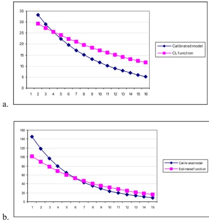
Sandström (1996). We compare the resulting functions with the CL functions estimated on the raw data in the original studies.

The marginal functions (value of increasing visibility by one metre at different sight depths) for the calibrated model and the estimated functions from the original studies are shown in

Figure 1. For both travel cost studies, a γ value of 0.8 was found to best mimic the original

functions. We chose not use the original functions directly because they are estimated for data that cannot be obtained from general data sources for the policy sites.

(15)

a. 0 5 10 15 20 25 30 35 1 2 3 4 5 6 7 8 9 10 11 12 13 14 15 16 Calibrat ed model CL f unct ion b. 0 20 40 60 80 100 120 140 160 1 2 3 4 5 6 7 8 9 10 11 12 13 14 15

Calibr ated model Estimated f unction

Figure 1. Marginal value of increasing visibility. Estimated conditional logit functions function vs. calibrated models after a) Soutokorva (2005) and b) Sandström (1996).

For coastal areas, we aggregate by transferring the value from one county to all other coastal counties in Sweden, correcting for differences in water quality and income levels, and then adding them up. We assume this transfer from the available county-specific studies is valid for all other coastal counties in Sweden. The valuation studies used seemed well suited for this purpose. The population in the CV studies used include both users and non-users from the adjacent counties and is representative of the country populations. The respondents in the TC studies also came from areas in the adjacent counties. Income levels differ between counties, which is corrected for in the transfer.

Other important aspects for the validity of the transfer are similarity of sites and quality changes, as well as availability of substitutes. Whether or not a given sites can be viewed as similar depends upon the site you use for comparison. Coastal areas in Sweden are fairly similar (in particular if one excludes the northern areas), in relation to the Mediterranean or the Atlantic coast. On the other hand, there are several dissimilarities between the west and the east coast of Sweden, such as the salinity of the water and the character of the

(16)

archipelagos. However, the available study estimates from the west and the east coast were very similar for the same quality change. The coastal counties studied are large and

encompass different types of sites (archipelagos, beaches etc). All counties have areas that are attractive for recreation.

The studies used (Soutokorva 2005, Söderqvist & Scharin 2000) valued an approximate one meter change of sight depth (from 2.3 to 3.4 meters based on a secchi disc reading). Data on sight depth as well as reference sight depth (corresponding to water quality of class 1) for each area are available from the county administrations and the Swedish EPA (for sources, see Table A1 in appendix A).

No freshwater studies from Sweden were available. Instead, we rely on valuation studies from adjacent countries in Northern Europe. These studies estimate the value of improving water quality in a lake or watercourse. They were similar in design and valued a quality change in terms of moving from one quality class to another. Water quality was classified on a five-level scale based on total phosphorus content. The description of quality classes include turbidity, algae growth and oxygen levels. Respondents were local residents. The availability of similar substitutes is not reported for all the studies. The Orre and Vansjö-Hobol lakes in Norway are reported to have no similar substitutes in the surrounding area, while

Steinsfjorden is reported to have at least one substitute. The size of the lakes vary considerably, from 1 to 900 km2, the median being 10 km2.

There are lakes larger than 10 km2 in each of Sweden's counties and in all but two counties there are lakes larger than 100 km2 (SMHI, 2008). Eutrophication levels vary across the country. Computations are done given the average quality and income level in each county. The assumption made is that the population in each county is prepared to pay for reducing eutrophication in one (1) lake or freshwater course, in relation to the eutrophication level in that country. The values for each county are subsequently aggregated to a value for the whole country. Assuming that the transfer is valid, the aggregation is likely to be a conservative estimate, since the quality levels used are an average for each county, so there will be lakes that have lower quality. The inhabitants may however be willing to pay for reducing eutrophication in more than one lake or watercourse, or none,, which is not taken into account. This may lead to either an under- or an overestimation.

(17)

2.2 Allocating damage values to pollutants: empirical issues

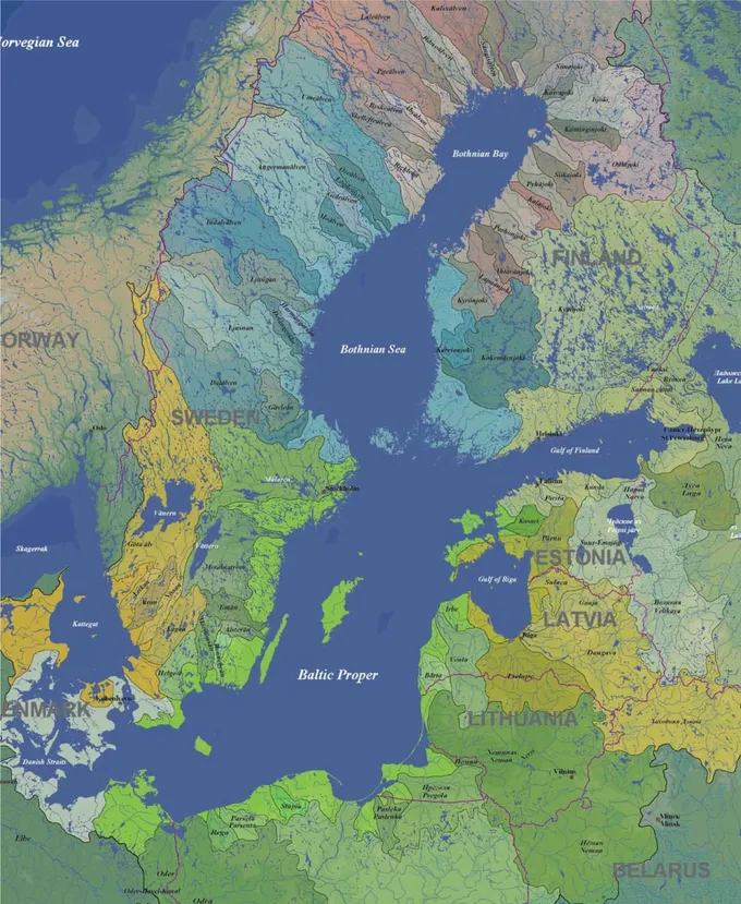
The Baltic Sea (Figure 2) has long been affected by eutrophication, due to high levels of nitrogen and phosphorus entering the system. The emissions originate from all countries adjacent to the Baltic, and also via air deposition from other European countries, such as the UK. Among the impacts of eutrophication are turbidity, reduced sight depth, more algae blooms in spring and summer and less biodiversity (Swedish EPA, 2005). Blooms of

Cyanobacteria (often called toxic blue-green algae) are an increasing problem, with the most severe occurrence in the summer of 2005 (Länsstyrelsen i Stockholms län, 2006).

In the last few years there has been a lively debate on the influence of nitrogen and

phosphorus on the eutrophication of the Baltic, with some experts claiming too much focus on reducing nitrogen, resulting in too little effort to reduce phosphorus (Boesch et al., 2006 ). This is important for reducing Cyanobacteria (or blue-green algae) blooms, which are a considerable problem in the east coast. Phosphorus concentration is the limiting factor for Cyanobacteria growth since they fix nitrogen from the air (i.e., they are not dependent on nitrogen content in the water). However, for other algae blooms in the spring, nitrogen is the limiting factor (Swedish EPA, 2005). Moreover, the situation differs between the west and east coast of Sweden. On the west coast, reduction of nitrogen emissions is more important than on the east coast. On the east coast, opinions differ on the importance of nitrogen reduction for improving water quality in the Baltic. According to some experts, nitrogen reductions are more important than phosphorus reductions for the inner archipelagos, while the opposite is true for the open sea (Boesch et al, 2006, Gothenburg University 2008). The Gulf of Bothnia is not as affected by eutrophication as the Baltic, and nutrient loads are also lower there (Swedish EPA 2005, Boesch et al., 2006 ).

(18)

Figure 2. The Baltic Sea.

To relate the derived damage values to the causing pollutants, the total damage value for each ecosystem is divided by annual deposition of each pollutant. However, since one kilogram of nitrogen (N) does not have the same eutrophying effect as one kilogram of phosphorus (P), the deposition of each pollutant needs to be weighted by its eutrophying potential in different ecosystems. As discussed above, a scheme for developing these weights is not self-evident

(19)

and may differ between ecosystems. Ideally, a dose-response function would be needed to allocate the eutrophication damage to N and P. The Department of Systems Ecology at Stockholm University estimated this type of function for sight depth in the Baltic Proper (Söderqvist and Scharin, 2000). They found that P was not significant in their estimation.

Thus, applying this function would allocate the entire estimated damage value exclusively to nitrogen. However, for the eutrophication of the Baltic, it is clear that phosphorus plays an important role (Boesch et al, 2006). Sandström (1996) carried out a simple regression for sight depth on N and P concentrations from three municipalities and found that both

pollutants were significant. The estimated weights were 78 percent for N and 22 percent for P. These functions only address the linkage between sight depth and nutrient concentrations. If Cyanobacteria blooms are taken into account, a much higher weight should be given to phosphorus than in the above-mentioned functions, which consider only sight depth.

There are generic characterisation factors that estimate the eutrophication potential of nitrogen and phosphorus, similar to the Global Warming Potential (GWP) for greenhouse gases.

According to the standard set in the Handbook on Life Cycle Assessment, the operational guide to the ISO standards (Guinée, 2002), one kilogram of P has seven times more

eutrophying potential than one kilogram N. This is a generic value for emissions to air, water and soil. This relationship coincides with the so-called Redfield ratio (Redfield 1963), which has been found to be appropriate for use in the Gulf of Finland (Kiirikki et al, 2003).

In these calculations, we will follow the method used by Helcom (Kiirikki et al 2003) and use the generic characterisation factors. We provide sensitivity analyses showing results using different allocation methods in section 6.

Eutrophication of land ecosystems like forest and meadow lands lead to higher biological production, changed species composition and, in some cases, reduced biodiversity. Species that are adapted to nutrient-low environments may be crowded out. However, these aspects are not included in the damage values because the valuation studies concern only

(20)

For the case of acidification from different pollutants, we apply an approach similar to the eutrophication adjustment . In NIER (1998), approximately 67 percent of the damages from acidification are allocated to sulphur and the remaining 33 percent to nitrogen. This

assumption is based on expert assessments from the Swedish EPA (personal communication). In the Handbook on Life Cycle Assessment (Guinée, 2002), best estimates of the acidification potential of SO2, NOx and NH3 are set at 1, 0.7 and 1.88, respectively. However, these

characterisation factors are not well suited for Sweden, where nitrogen retention is much higher (leading to reduced acidification impacts). Taking into account both the considerations in NIER (1998) and statements on the website of the Swedish NGO Secretariat on Acid Rain (www.acidrain.org), we believe that the NIER values best reflect the acidification impact of the pollutants in Sweden. Sensitivity analyses showing results for alternative characterisation factors are given in section 6.

3. Results

3.1 Total damage values

Eutrophication of coastal areas

Eutrophication of coastal areas in Sweden has been valued in several Swedish studies. Söderqvist and Scharin (2000) and Soutukorva (2005) estimated the value of halving

emissions to the Stockholm archipelago, corresponding to an improvement of the sight depth from two to three meters. Water clarity is linked to eutrophication levels in different quality class systems (see e.g. Swedish EPA, 1999; Norwegian State Pollution Control Agency, 2003). It is also an observable feature that influences people’s experience of the sea, which is why sight depth is often used as the describing variable for marine areas.

The Swedish travel cost studies Sandström (1996) and Soutukorva (2005) both value an increased water quality in terms of reduced nutrient concentrations. Both used sight depth as the indicator for water quality. In Sandström (1996) the study concerned water quality along the entire Swedish coast and therefore includes all Swedish residents in the survey population. The study relied on a national database, but information about short trips (e.g. day trips to the local beach) was not included. Soutukorva (2005) valued increased water quality in the

(21)

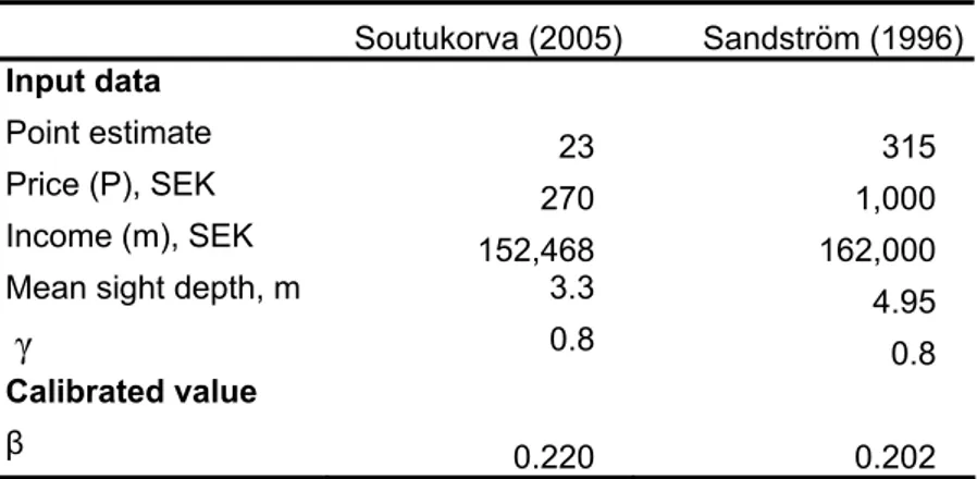
Stockholm archipelago, a relatively small and well-defined area in the vicinity of Stockholm. In that study, short trips were included. The survey population included the two counties adjacent to the archipelago. Inserting data from the two studies in equation (9), β values were calibrated. Input data and the calibrated β values are shown in Table 1.

Table 1. Input data and calibrated β values from two travel cost studies.

Soutukorva (2005) Sandström (1996)

Input data

Point estimate _{23 315}

Price (P), SEK _{270 1,000}

Income (m), SEK _{152,468 162,000}

Mean sight depth, m 3.3 _4.95

γ 0.8 _0.8

Calibrated value

β _{0.220 0.202}

For the purpose of this analysis we will use the β value calibrated from Soutukorva (2005) for the coastal areas because this study addresses a local population and a confined area. Further, the local pollution sources are likely to be of high importance in determining water quality. Mean travel cost (P) and the calibrated β value was inserted into eq. (1) together with county-specific values of income (m) and water quality (q). This transfer function was then used to compute damage values for other regions and water quality levels.

Given the current regional water quality class of the coastal counties in Sweden, we are able to calculate the value of restoring each coastal zone to a non-eutrophied state for that zone (as defined by the Swedish EPA, see Table A1 in Appendix 1). The estimates are adjusted for income differences between the counties (SCB, 2007). Data on current water quality status are taken from county annual reports (sources, see Table A1). The total value is seven billion Swedish Kronor (SEK), which corresponds to an average value per inhabitant of 1,400 SEK.

Eutrophication of the Baltic Sea

In addition to the water quality along the Swedish coast, we also consider the eutrophication status of the Baltic Sea as a whole because it too has value for coastal residents. Söderqvist (1996) estimated the basin-wide value for increasing visibility in the Baltic Sea from 5 to 8.7

(22)

metres, which represents a water quality with almost no eutrophication. This quality change was assumed to be achieved by halving nutrient deposition to the Baltic through reducing emissions from all countries in the drainage basin. The WTP in Sweden for this quality change was estimated at 2,500 SEK per person per year, inflated to 2005 year value using a 4 percent discount rate. All values presented in this paper are in 2005 SEK values unless otherwise noted. This amounted to a national aggregate of 17 billion SEK. The total value for residents in other countries around the Baltic Sea estimated in 1996 is equal to approximately 23 billion SEK in 2005 value.

Eutrophication of freshwater

For eutrophication of freshwater, studies from adjacent countries were used since there were no Swedish valuation studies available (Table 2). The studies are from other north and western European countries that have a similar natural environment to Sweden and a similar use-pattern, with fishing and swimming being common activities (other common activities are sunbathing and walking along the lake, see Methodex 2007a).

The studies all valued a one-class improvement in water quality using a five-step water quality ladder (Norwegian State Pollution Control Agency, 1989). In freshwater, visibility is very much affected by the content of humus and organic material in the water; thus, sight depth may not be suitable as the only indicator for eutrophication in freshwater. The water quality ladder include indicators for visibility, oxygen, algae growth, living conditions for salmon and frequency of algae blooms. The resulting water quality is interpreted in terms of the water´s suitability for drinking, bathing, irrigation, recreational fishing and boating. The initial quality class - as well as the end quality level reached - differed among the studies. This is taken into account in the calibration.

(23)

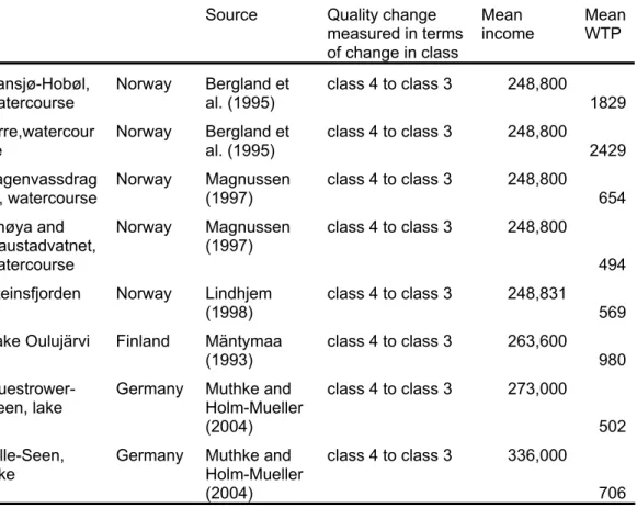
Table 2. Mean point estimates from Scandinavian and German CV studies on reducing eutrophication of freshwater (2005 SEK values)

Source Quality change

measured in terms of change in class

Mean

income Mean WTP Vansjø-Hobøl,

watercourse Norway Bergland al. (1995) et class 4 to class 3 248,800 1829 Orre,watercour

se Norway Bergland al. (1995) et class 4 to class 3 248,800 2429 Lagenvassdrag

et, watercourse Norway Magnussen (1997) class 4 to class 3 248,800 654 Ånøya and Gaustadvatnet, watercourse Norway Magnussen (1997) class 4 to class 3 248,800 494 Steinsfjorden Norway Lindhjem

(1998) class 4 to class 3 248,831 569

Lake Oulujärvi Finland Mäntymaa (1993)

class 4 to class 3 263,600

980

Guestrower-Seen, lake Germany Muthke Holm-Mueller and (2004)

502 Ville-Seen,

lake Germany Muthke Holm-Mueller and (2004)

706

Converted to SEK using PPP adjusted exchange rates (www.oecd.org/dataoecd/61/56/1876133.xls)

We estimated benefit transfer functions for each of these sites by inserting data on income and WTP values from each study into eq. (1), together with the β value estimated from

Soutukorva (2005). The α values calibrated from the different studies are shown in Table 3. To illustrate the difference in WTP estimates implied by different values of α , WTP for a one-class quality change (from class 3 to class 2) is also shown (Table 3). The values are calculated with mean Swedish income for 2005 (Statistics Sweden, 2007).

(24)

Table 3. Parameter values for transfer functions calibrated on CV studies from Scandinavian countries. WTP estimate for Sweden for a water quality increase from class 3 to class 2, using transfer function with Swedish mean income level 2005. β = 0.22

Study site α (SEK) WTP

Vansjö-Hoböl 0.029 1,844 Orre 0.038 2,439 Lagenvassdraget 0.010 658 Ånøya 0.008 497 Steinsfjord 0.008 518 Randers fjord 0.014 895 Lake Oulujärvi 0.013 840 Guestrower-Seen 0,007 442 Ville-Seen 0,008 505

Sources: see Table 2.

The benefit transfer functions yield values that range from 440 to 2,430 SEK for improving water quality from class 3 to class 2. As can be seen from Table 3, the estimates from Orre and Vansjö-Hobol lie considerably higher than the other locations, as has been noted in several benefit transfer studies (e.g., Muthke and Holm-Muller 2004, Methodex 2007a). They both represent large lakes (8 and 37 km2_{, respectively) without similar substitutes nearby. The}

mean α value is 0.015 if Orre and Vansjö-Hobol are included, and 0.010 otherwise. This corresponds to a WTP value for an improvement from class 3 to class 2 of SEK 965 and 645, respectively. Since substitute sites are likely to be available in most Swedish counties (SMHI 2008), we will use the lower α value of 0.010 and perform a sensitivity test using the higher α value.

Damage values for each of Sweden’s 21 counties are computed (see Table A3 in Appendix 1) using eutrophication mappings for each county (Swedish EPA, 1995) and adjusted for

income. The national aggregate amounted to 3 billion SEK, which corresponds to an average of 450 SEK per person.

Nitrate in groundwater

High nitrate (NO3) content in drinking water is carcinogenic and causes health problems to

infants. These impacts have been valued by Silvander (1991) and NIER (1998). Both studies give a value of around 330 SEK per person per year to avoid nitrate levels in groundwater above recommended limits. This is equal to a total value of 2.9 billion SEK per year at 2005 values (aggregating for the population between 18 and 64 years of age).

(25)

Acidification

For acidification, few valuation studies exist in Europe. There are no studies where the willingness to pay is related to a quality measure. The valuation study that encompasses most of the impacts of acidification in Sweden is NIER (1998). In that study, respondents were asked to state their willingness to pay to eliminate acidification of all lakes and forests in Sweden through emission reductions and prudent liming of some heavily acidified lakes and forest areas. The estimated average value was 890 SEK per person per year for eliminating acidification of freshwater lakes and watercourses, and 420 SEK per person per year for eliminating acidification of forests. In total, this amounted to 8.7 billion SEK for the population aged between 18 and 64 years.

3.2 Generic damage values per pollutant

In order to use the damage data in tools such as CBA and LCA, and for modelling exercises with economic models, damage values are best expressed per kilogram of pollutant. The procedure for allocating values per pollutant requires a distribution of the eutrophication and acidification impacts to the substances responsible.

To avoid double counting when aggregating values to the national level, we treat the values for the coastal areas and the Baltic as partially overlapping for inhabitants in coastal counties. Thus the value per person for overall water quality enhancement in the Baltic was reduced by the value for local water quality enhancement for inhabitants in coastal counties. Inhabitants in inland counties were only ascribed the value for the Baltic water quality improvement. Northern counties were ascribed only the value for reducing eutrophication in the entire Baltic Sea, since the Gulf of Bothnia is not as affected by eutrophication as the Baltic Proper and the western seas (Boesch et al., 2006). The damage value per kilogram for pollutants deposited by the coast becomes higher than the value per kilogram of pollutants deposited outside Swedish coastal waters because the reduction of nutrients needed to enhance water quality at a

confined coastal area is smaller than the reduction needed to enhance quality in the Baltic as a whole. For nitrogen and phosphorus deposited in the Baltic Sea, there is also a value

associated with water quality improvements for inhabitants in other countries that border the sea. These values are taken from Söderqvist (1996)and allocated to the eutrophying

(26)

substances. Table 4 shows the total damage values computed for the relevant population. The values for coastal areas and freshwater are derived from the county calculations (see Tables A1 and A3 in the Appendix).

Table 4. Total damage values for eutrophication of water and acidification

Total value, billion SEK Eutrophication of the Baltic

Swedish population, for local coastal areas1 7 Swedish population, for entire Baltic Sea1 10

Other inhabitants around the Baltic2 ₂₃

Eutrophication of freshwater1 ₃

Nitrate in groundwater3 2.9

Acidification3 8.7

1_{Own calculations (see Table A1, A2 and A3 in Appendix 1)}

2_{Söderqvist (1996)}

3_NIER(1998)

The total damage values are allocated to the pollutants responsible in order to obtain the damage value per kilogram of pollutant. For eutrophication of the sea, we use the

characterisation factors mentioned in section 2.2. For freshwater, the eutrophication values are allocated only to phosphorus because phosphorus is the limiting substance in lakes and rivers in Sweden. Thus, nitrogen deposition does not have any impact on eutrophication levels (Swedish EPA, 2003a).

The damage from nitrate in drinking water is allocated to different nitrogen compounds in proportion to their share of nitrogen deposition. Annual deposition of nitrogen emissions to air is about 130 thousand tons (kton) (Swedish EPA, 2003a) and emissions to freshwater are about 102 kton (Swedish EPA, 2007). The average retention rate of nitrogen deposited in soil and lakes is about 30 percent, while the retention in watercourses is negligible (Swedish EPA 2002, TRK 2007). Taking account of the retention to estimate the nitrogen load to

groundwater, the damage value amounted to 9 SEK per kilogram nitrogen. The values for NO3 and NH3 to groundwater are computed in the same way.

The main acidifying substances are sulphur dioxide (SO2), nitrogen oxides (NOx) and

ammonium (NH3). As discussed in section 2.2, the total damage value for acidification is

allocated to these substances using expert assessments, where the acidification potential of sulphur is about twice as large as that of nitrogen.

(27)

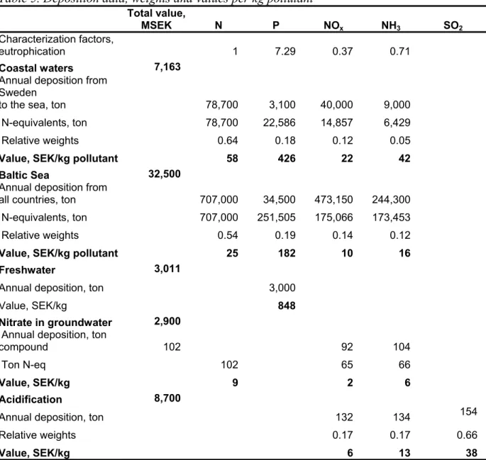
The total damage values shown in Table 4 are allocated to different pollutants as described above and divided according to deposition of each pollutant. Input data and resulting values per kilogram of pollutant are shown in Table 5. The calculations are based on deposition data for the Baltic from HELCOM (2005b) and for Swedish coastal waters and freshwater systems from Swedish EPA (2003a).

Table 5. Deposition data, weights and values per kg pollutant

Total value,

MSEK N P NOx NH3 SO2

Characterization factors,

eutrophication 1 7.29 0.37 0.71

Coastal waters 7,163

Annual deposition from Sweden

to the sea, ton 78,700 3,100 40,000 9,000

N-equivalents, ton 78,700 22,586 14,857 6,429

Relative weights 0.64 0.18 0.12 0.05

Value, SEK/kg pollutant 58 426 22 42

Baltic Sea 32,500

Annual deposition from

all countries, ton 707,000 34,500 473,150 244,300

N-equivalents, ton 707,000 251,505 175,066 173,453

Relative weights 0.54 0.19 0.14 0.12

Value, SEK/kg pollutant 25 182 10 16

Freshwater 3,011

Annual deposition, ton 3,000

Value, SEK/kg 848

Nitrate in groundwater 2,900

Annual deposition, ton

compound 102 92 104

Ton N-eq 102 65 66

Value, SEK/kg 9 2 6

Acidification 8,700

Annual deposition, ton 132 134 154

Relative weights 0.17 0.17 0.66

Value, SEK/kg 6 13 38

Deposition data: (Swedish EPA, 2003, 2004, 2007; HELCOM, 2005); characterisation factors: (Guinée, 2002).

Regional values can also be computed using local deposition levels. Table 6 shows both the national average and values for one kilogram of pollutant deposited in two regions of different sizes, namely the southern drainage basins and the Stockholm archipelago. The regional

(28)

values were calculated using the site-specific values derived here (see Table A1 in Appendix) and deposition data from Swedish EPA (2003a) and Söderqvist and Scharin (2000). As can be seen, the values vary widely for different regions. This is due to the differences in quality levels, numbers of people affected and the deposition of pollutants in each area. The high value per kilogram deposited in the Stockholm archipelago is mainly due to the fact that it is a densely populated area.

Table 6. Damage value for eutrophication of the sea. SEK per kg

N P NOx NH3

Average for all drainage basins around

Sweden 83 608 31 60

South drainage basins 93 528 35 67

Stockholm archipelago 238 1,212 63 39

The values derived here refer to pollutants that end up in freshwater, coastal water and the Baltic Sea and, for the case of acidification, deposited in forests. To calculate generic values for pollutants emitted elsewhere in Sweden, these values are corrected for the average fraction of Swedish emissions that end up in the respective ecosystem area. Thus, the value of nitrogen emissions to air was weighted with the percentage that is deposited in the Baltic sea, which is about 16 percent (EMEP, 2000a). This decreases the value of NOx to about 3 SEK and the

value of NH3 to about 5 SEK. The remaining 84 percent of N emissions are deposited on soil.

This part was valued using the damage value for nitrate and acidification. About 20 percent of sulphur emissions in Sweden end up in the Baltic Sea or the Atlantic, giving a weight of 0.8 for the sulphur value (EMEP, 2000b). The average retention rate of nitrogen emissions to soil and water is about 30 percent (TRK 2007). The value for nitrogen was thus weighted at 0.7. The resulting generic values obtained are presented in Table 7.

Some fractions of the Swedish emissions end up in other countries. Ideally, models of emission transport should be used together with valuation of the damage they cause in different regions. Instead, we use a simplified approach, assuming that the damage value due to nitrate and acidification is as large in other countries as it is in Sweden. Thus, the fraction of the emissions that do not end up in the sea are valued using the damage values derived for Sweden.

(29)

Table 7. Generic damage values (SEK) for sulphur, nitrogen and phosphorus per kg pollutant. Site-independent average

N P NOx NH3 SO2

Eutrophication of the sea 83 608 31 60

Weight 1 _{0.7 0.75 0.16 0.16} Generic value 58 456 5 10 Eutrophication of freshwater 848 Weight 1 _0.25 Generic value 212 Nitrate in groundwater 9 2 6 Weight 1 ₁ _{0.84 0.84} Generic value 9 2 5

Generic value eutrophication 67 668 7 15

Acidification 6 13 38

Weight 2 0.84 0.84 0.8

Generic value acidification 5 11 30

Total generic value SEK/kg 67 668 12 26 30

1_Nitrogen: _{Retention rates from TRK(2007) and transport data from EMEP (2000a) Phosphorus: estimates from} Swedish EPA (2004)

2 _{Transport data from EMEP (2000b).}

4. Uncertainty

Since there are no markets for the environmental goods and services valued here we do not know the “true” marginal value attached to these amenities. The valuation methods used here give one estimate of the welfare loss. One way to test whether these values are representative of the populations’ valuation of the amenities is to compare these values with other studies that value the same goods. Even if there are several such studies available, we do not know which study comes closest to the “true” value. The relative standard error in the original studies lies between 2 and 8 percent of the WTP values (Söderqvist 1996, Söderqvist and Scharin 2000, Soutukorva 2005). In addition to the uncertainty of the valuation studies, the practice of benefit transfer also involves transfer errors. These are

equally difficult to assess, since original values are missing. Below we will discuss transfer errors by comparing with available studies and discuss some of the assumptions made in the derivation of the generic values.

We were able to make a simple estimate of the transfer error for the function from the

Stockholm archipelago by comparing it with a similar study available for the Laholm Bay on the south-west coast of Sweden. The Stockholm archipelago is a popular tourist area and lies in a densely populated part of the country, where prices and wages are higher than in more

(30)

rural parts of the country. A higher willingness to pay in this area could therefore be expected. Frykblom (1998) estimated WTP for reduced nutrient emissions to the Laholm Bay on the south-west coast of Sweden. The quality change was described as moving from quality class 4 to class 2, which corresponds approximately to a sight depth change from 2.5 to 4 metres (Swedish EPA, 1999). Mean annual WTP was estimated at 820 SEK (discounted present value). The value for this quality change calculated with the transfer function derived above is 850 SEK when the income level in the transfer function was adjusted to the level in Laholm. The error rate can be calculated with a formula suggested in Kirchoff et al. (1997):

(WTPtransferred-WTPpredicted)/WTPpredicted) where WTPpredicted is the estimate from the

site-specific study, in this case the Laholm study. The error rate between Stockholm and Laholm is 4 percent.

The transfer errors for the freshwater sites used above have been tested (Ahlroth,

forthcoming) and found to range between 0 and 55 percent when using a medium estimate of the calibration parameter (α). As mentioned in section 4.3, the estimated damage values in the Norwegian studies for Orre and Vansjö-Hobol were “outliers” in the set of valuation studies. Including them in our calculations, which changes the α value from 0.010 to 0.015, increases the total damage value from 3 to 4.6 billion SEK. This changes the damage value for

phosphorus from 850 to 1,300 SEK/kg, which is about 50 percent higher.

There is no similar study with which to compare the basin-wide value of reducing

eutrophication. The population mean WTP chosen is a conservative estimate (Söderqvist, 1996). This is also the case for the WTP value used for the estimates in coastal areas

(Söderqvist and Scharin, 2000). To get an idea of the total uncertainties involved, we made a rough estimate using assumptions about the error rates based on the discussion above. If a 100 percent error rate is used for the basin-wide values, 10 percent for coastal values and 60 percent for the freshwater values, the error range of the values for N and P becomes around 40 percent. This, of course, excludes the uncertainties inherent in the valuation studies

themselves.

In our calculation of damage values, we have chosen the allocation method tested for a part of the Baltic Sea by Kiirikki et al. (2003). To illustrate how a different allocation could influence

(31)

the damage values we calculate damage values using an ad hoc-function derived in Sandström (1996). The function is derived by making a simple regression on sight depth and nutrient concentration data for different areas in the Stockholm archipelago.

To illustrate the impact of the assumptions for allocating the total damage values to different pollutants, we show the values per kilogram of pollutant using different assumptions in Tables

8 and 10.

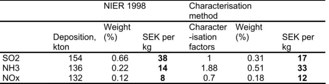
In Table 8, different allocation factors for acidification are shown. The weights from NIER (1998) are based on expert assessments. In the ‘characterisation method’, NOx and NH3

deposition is converted to SO2 equivalents using characterisation factors from Guinée (2002),

and relative weights are calculated from the respective pollutant’s fraction of the total SO2

equivalents. As can be seen in the table, the relationship between sulphur and ammonia shifts when the characterisation factors are used instead of the NIER weights.

Table 8. Acidification: damage values for SO2 , NH3 and NOx using different weights (2005

SEK values) NIER 1998 Characterisation method Deposition, kton Weight (%) SEK per kg Character -isation factors Weight (%) SEK per kg SO2 154 0.66 38 1 0.31 17 NH3 136 0.22 14 1.88 0.51 33 NOx 132 0.12 8 0.7 0.18 12

Sources: Weights and characterisation factors from Guinée(2002) and NIER (1998); deposition data from Swedish EPA(2003c).

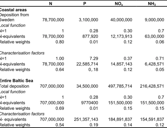
Table 9 shows the relative weights for eutrophication that results from using characterisation

factors from Guinée (2002) and the ad hoc-function estimated by Sandström (1996) for

Stockholm archipelago (see section 2.2). The relative weight corresponds to the fraction of the total damage ascribed to each pollutant. For nitrogen, the weight using alternative methods lies between 54 and 80 percent, while the weight for phosphorus lies between 1 and 19 percent.

(32)

Table 9. Deriving relative weights for different allocation methods N P NOx NH3 Coastal areas Deposition from Sweden 78,700,000 3,100,000 40,000,000 9,000,000 Local function N=1 1 0.28 0.30 0.7 N-equivalents 78,700,000 877,920 12,173,913 63,00,000 Relative weights 0.80 0.01 0.12 0.06 Characterisation factors N=1 1.00 7.29 0.37 0.71 N-equivalents 78,700,000 22,585,714 14,857,143 6,428,571 Relative weights 0.64 0,.18 0.12 0.05

Entire Baltic Sea

Total deposition 707,000,000 34,500,000 497,785,714 216,428,571 Local function N=1 1 0.28 0.30 0.7 N-equivalents 707,000,000 9770400 151,500,000 151,500,000 Relative weights 0.69 0.01 0.15 0.15 Characterisation factors N- equivalents 707,000,000 251,357,143 184,891,837 154,591,837 Relative weights 0.54 0.19 0.14 0.12

Table 10 shows the calculation of damage values using the local allocation function or the

generic characterisation factors for both coastal waters and the entire Baltic Sea. Since the damage value is divided over a smaller amount for phosphorus than for nitrogen, the difference in damage value per kilogram differs more for phosphorus. The estimate for phosphorus using the ad hoc function for the Stockholm Archipelago is about 5 percent of the estimate using characterisation factors. This reflects the low effect on visibility from

phosphorus found in the regression in Sandström (1996). The value for nitrogen when using the ad hoc function is about 25 percent higher than the value calculated with characterisation factors. Accounting for the relatively widespread expert opinion that reducing nitrogen is more important in coastal waters than reducing phosphorus- and vice versa for the algae blooms in the open sea - a possible choice could be to use the method putting less weight on phosphorus for coastal waters and the method putting more weight on phosphorus for the values of the entire Baltic Sea, which is dominated by open sea. The last row in Table 10 shows the values using this mixed allocation. Combining with the values for eutrophication of freshwater, the value per kilogram P ranges between 880 and 1,450, a difference of about 60 percent.

(33)

Table 10. Eutrophication of the sea: damage values for N , P, NOx and NH3 using different

weights (2005 SEK values)

N P NOx NH3

Local function for all areas 105 30 32 73

Generic characterisation factors for all areas 83 608 31 60

Local function for coastal areas, generic

characterisation factors for the entire Baltic Sea 98 203 32 69

5. Comparison with Swedish tax rates and avoidance cost estimations

The purpose of environmental taxes is to internalise external effects from different activities. Given the damage values derived above, how do the Swedish environmental taxes perform in this regard?

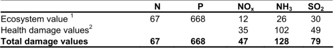
Table 11. Generic ecosystem damage values and health impact values. SEK/kg

N P NOx NH3 SO2

Ecosystem value 1 67 668 12 26 30

Health damage values2 35 102 49

Total damage values 67 668 47 128 79

1_{From Table 7} 2 _{Methodex (2007b)}

It seems as though the Swedish tax rate on sulphur dioxide, 30 SEK per kg is supported by the ecosystem damage values, but the fee on nitrogen in fertilisers, 1.80 SEK per kg nitrogen (Swedish EPA 2003b), is too low according to our derived values of the ecosystem damage (see Table 11). There is a fee of 40 SEK per kg nitrogen oxide emission to air, which is higher than the ecosystem damage value for nitrogen oxides, but in the same magnitude as the total value including health effects. Since this fee only applies to larger furnaces in power plants, it seems that the economic incentives to reduce nitrogen emissions in Sweden are not on par with the public's value of reduction.

Costs for abating emissions of sulphur, phosphorus and nitrogen compounds have been compiled within the MARE project and has been employed in studies for HELCOM. Compilations of costs for reducing nitrogen emissions in Sweden can be found in Elofsson and Gren (2003) and Eklund (2005). Table 12 shows average cost per reduced kilogram nitrogen.

(34)

Table 12. Costs for reducing nitrogen emissions to air and water, at the source and deposited by the coast.

Measure

Average cost per reduced kg N (SEK/kg)

At the source By the coast Measures in coastal

industry1 48 48

Measures in sewage

treatment plants1 48 62

Nutrient catch crops1 81 100

Reduced use of fertilizers1 10 15

Wetlands1 ₃₆ ₄₅ Measures against ammonia leakage in agriculture2 ₄₀ ₁₅₁ Catalytic converters in private cars2 97 552

Measures abroad1,a 9 13

1_{Emissions to water} 2_{Emissions to air}

a_{Sewage treatment plant projects in Baltic countries} Source: Elofsson and Gren (2003), Eklund(2005)

The benefit of reducing nitrogen deposited to the sea is calculated to be between 80 and 105 SEK/kg nitrogen, using the span calculated in the sensitivity analysis with different allocation methods. Adding an uncertainty range of 40 percent, the value of nitrogen can vary between 50 and 150 SEK/kg. Even when the lower limit is considered, most of the measures targeting emission to water would pass a cost-benefit test. The cost of growing catch crops, however, may be higher than the benefits. Measures against leakage of ammonia in agriculture may have a positive net benefit, depending on where the measures are taken. Requiring catalytic converters is not an efficient measure for reducing eutrophication of water - not surprisingly since so little of these emissions (16 percent) are deposited in the sea.

Abatement costs for phosphorus emissions have been calculated for reducing phosphorus emissions from different activities within the drainage basin of a relatively large lake in the middle of Sweden, Glan. These cost estimates have been used in economic assessment of the Swedish national environmental objective "Zero Eutrophication."

Abatement costs per kg phosphorus are high compared to the benefits estimated in this paper. The benefit of reducing one kg of phosphorus is estimated at 600 SEK/kg when targeting emissions ending up in the sea. Including an uncertainty range of 40 percent, the span

(35)

becomes 350-850 SEK/kg. For impacts from P emissions ending up in freshwater, the damage value amounted to 850 SEK/kg. A site-independent average was calculated to be about 670 SEK/kg for phosphorus. As can be seen from Table 13, few measures cost less per kg than the estimated benefits. In the agricultural sector, growing crops that bind phosphorus is an option that may be warranted. In sewage treatment plants, several measures can be taken that may have a positive net benefit. To connect private sewage systems to the municipal sewage systems is, however, on average a costly measure that is not warranted by the reduction of phosphorus emissions alone.

Table 13. Costs for reducing phosphorus emissions in the drainage basin of the Swedish lake Glan.

SEK/kg P Agriculture Energy crops 0 - 1,000

Grass on headlands 800-4,500 Wetlands/dams 1,500-5,000 Protection zones 5,000-30,000 Private sewage systems Infiltration bedding 4,000-5,600 Connection to municipal sewage systems 6,000 Sewage treatment plants Process optimisation 1,450-3,000 Sand filters etc 900-1,250

Wetlands/dams 700-1,700

Vegetation

filters 700-

Surface water Wetlands/dams 2,000-2,500

Source: Swedish EPA (2004).

6. Discussion

The calculated damage values attempt to illustrate the value attached to better environmental quality in terms of decreased eutrophication and acidification in Sweden. It is important to note that the values derived for eutrophication only include the impacts on water. Terrestrial eutrophication is not included, which means that the value for nitrogen is an underestimate. The impact on marine and freshwater biodiversity from acidification and eutrophication is however implicitly included, since the valuation surveys include descriptions of how the ecosystems might be affected in this regard. The impact on fish stocks is included in the same

(36)

way. Valuation studies of recreational fishing in Sweden (e.g. Paulrud 2003a, 2000b) have valued a change in fish catch, but this is difficult to link directly to environmental quality. Adding them to the values derived here could also give rise to double counting.

The assumptions made when calculating damage values for the substances involved in

eutrophication and acidification are conservative throughout. Despite this, we could conclude that the economic incentives to reduce nitrogen emissions in Sweden are not on par with the public's value of reduction.

Moreover, most abatement measures for nitrogen would have a positive net benefit according to these calculations. This is true also for the lower limit of the damage values. For some of the measures, the abatement costs lie within the limits of uncertainty. In these cases, the outcome of the analysis depends on the standpoint taken regarding the allocation of the damage of eutrophication between nitrogen and phosphorus.

For phosphorus, the situation is reversed. Most of the abatement measures are too costly compared to the benefits when only the effect on phosphorus emissions is considered.

However, some measures in sewage treatment plants and in agriculture might have a positive net benefit if the costs lie in the lower segment of the estimated cost span, or if less

conservative assumptions are made in the damage value calculations. Some measures, such as wetlands and dams, will reduce leakage of both nitrogen and phosphorus. If reduction of both nutrients is taken into account, this will enhance the cost-benefit ratio and may imply that some measures do have a positive net benefit.

It is also of interest to compare the derived damage values with the generic values for

eutrophying and acidifying pollutants used in cost-benefit analyses of infrastructure planning in Sweden. In the so-called ASEK projects, generic values for regional effects are derived (as opposed to local, which are based on ambient air pollution concentration and involve health effects). These values are based on abatement costs and are used as proxies for the total impact of these pollutants, i.e. health impacts, ecosystem impacts and other impacts (e.g. corrosion, crop yields). For our derived ecosystem damage values to be comparable with the ASEK costs, health impacts needs to be added. To this end, we use the generic health values

(37)

for Sweden from the BeTa database, produced in the EU project MethodEx, an off-shoot from the ExternE project (http://www.methodex.org/introduction.htm).

The value for SO2 is almost 50 percent larger than the ASEK cost estimate (Table 14), while

the generic value for NOx derived here is lower than the cost estimate in ASEK (though using

site-specific values can give quite different results, as shown in Table 6).

Table 14. Values (SEK/kg) for eutrophying and acidifying substances

N P NOx NH3 SO2

Damage values1

Eutrophication 67 668 7 15 0

Acidification 5 11 30

Health damage values2 _{35 102 49}

Total damage values 67 668 47 128 79

ASEK3 62 21

Ecotax024

Eutrophication 12 87 4 9

Acidification 15 48 30

1_{From Table 7}

2_{Source: BeTa – Methodex v1-07.}_{www.methodex.org/news.htm} 3_{Source:SIKA(2004)}

4_{Calculated from Finnveden et al.(2006), using characterisation factors from Guinée(2002).}

We also compare the values derived with values in a Swedish weighting scheme, Ecotax02 (Finnveden et al., 2006). In Ecotax02, tax rates and fees on pollutants in Sweden are used to derive weights per kilogram of pollutant. The method links a tax or fee to a relevant impact category. Even if the tax or fee is only expressed for one substance, characterisation factor conversion makes it possible to relate the value to substances that contribute to the same impact. In Ecotax02, the value for nitrogen is 12 SEK/kg and for sulphur 30 SEK/kg.

The Ecotax02 values for NH3, NOx and P are calculated using characterisation factors

(Guinée 2002). From Table 12, we can see that the ecosystem damage values put a higher value on eutrophication than Ecotax02, while they are lower for the acidifying impacts of nitrogen oxides and ammonia. The ecosystem damage value for sulphur happens to coincide with both the Ecotax02 value and the ASEK cost.