Camera pose estimation with moving Aruco-board. : Retrieving camera pose in a stereo camera tolling system application.

Camera pose

estimation with

moving Aruco-board

MAIN FIELD OF STUDY: Computer Science Embedded Systems AUTHORS: Jakob Isaksson, Lucas Magnusson

SUPERVISOR:Ragnar Nohre JÖNKÖPING 2020 April

Retrieving camera pose in a stereo camera tolling

system application

Mail Address:

Visiting Address:

Phone:

Box 1026

Gjuterigatan 5

036-10 10 00 (vx)

551 11 Jönköping

This thesis is performed at Jönköping University School of Engineering within [see main field of study on the previous page]. The authors themselves are responsible for opinions,

conclusions, and result. Examiner: Beril Sirmacek Supervisor: Ragnar Nohre

Magnitude: 15 hp (bachelor’s degree)

i

Abstract

Stereo camera systems can be utilized for different applications such as position estimation, distance measuring, and 3d modelling. However, this requires the cameras to be calibrated. This paper proposes a traditional calibration solution with Aruco-markers mounted on a vehicle to estimate the pose of a stereo camera system in a tolling environment. Our method is based on Perspective N Point which presumes the intrinsic matrix to be already known. The goal is to find each camera’s pose by identifying the marker corners in pixel coordinates as well as in world coordinates. Our tests show a worst-case error of 21.5 cm and a potential for centimetre accuracy. It also verifies validity by testing the obtained pose estimation live in the camera system. The paper concludes that the method has potential for higher accuracy not obtained in our experiment due to several factors. Further work would focus on enlarging the markers and widening the distance between the markers.

Keywords –Extrinsic camera calibration, OpenCV, Aruco, Perspective N Point, Tolling system.

ii

Acknowledgments

We would like to thank Kapsch TrafficCom AB and our supervisor Göran Boström for help throughout the thesis. We would also like to thank Beril Sirmacek and Ragnar Nohre from Jönköping University School of Engineering for their help and guidance during the process of writing this thesis.

We would also like to thank all the people involved that are not directly mentioned here that helped in different ways.

iii

Glossary

OpenCV Open Computer Vision

DOF Degrees of freedom.

Aruco A library for Augmented Reality applications based on OpenCV.

iv

1

Introduction ... 6

1.1 CONTEXT ... 6

1.2 PROBLEM STATEMENT ... 7

1.3 OBJECTIVE AND RESEARCH QUESTION ... 8

1.4 SCOPE ... 8

2

Method and implementation ... 9

2.1 OVERVIEW ... 9

2.2 STARTING POINT ... 9

2.3 APPROACH ... 9

2.4 CONNECTION BETWEEN RESEARCH QUESTION AND METHOD ... 13

2.5 DATA COLLECTION ... 13

2.6 DATA ANALYSIS ... 13

2.7 CREDIBILITY ... 14

3

Theoretical framework ... 15

3.1 ARUCO-MARKER DETECTION ... 15

3.2 PERSPECTIVE TRANSFORMATION ... 15 3.3 PERSPECTIVE NPOINT ... 16

4

Empirics ... 17

5

Analysis ... 22

6

Discussion and conclusions ... 23

6.1 RESULT ... 23

6.2 IMPLICATIONS ... 23

6.3 LIMITATIONS ... 23

v

6.5 FUTURE WORK ... 24

7

References ... 25

6

1

Introduction

1.1 Context

In many road applications, cameras are set up to monitor traffic. Depending on the use, the cameras could for instance measure distances and positions. This requires them to be

calibrated. The problem is finding a sophisticated calibration method providing high precision in an environment with constant traffic.

This paper will investigate the possibility to calibrate a tolling camera stereo system, using a vehicle driving through the gantry with a calibration pattern mounted on top. This is as opposed to traffic surveillance in urban areas [1] where the cameras often are mounted 15 meters or higher up to get an eagle-eye view over the traffic. However, our approach does have a height limit for when it no longer is viable. When the object becomes too small in the image plane, calibration patterns are no longer a feasible or reliable approach.

Our method is based on Perspective N Point (PnP), which is a way of calculating a camera pose with a known intrinsic matrix and object points. This will be further explained in 3.3. A camera pose is another word for the extrinsic matrix of a camera. It is also sometimes referred to as the 6DOF. It is the six degrees of freedom a camera has in a 3D coordinate system. That is, the location in x y and z as well as a rotation consisting of a pitch, yaw, and roll. In this paper, extrinsic parameters will be referred to as the camera pose.

The state-of-the-art methods for camera pose estimation today are to the best of our knowledge mostly self-calibration methods [2], [3] and [4]. Camera self-calibration is a collection name of methods utilizing objects naturally appearing in the camera’s image plane to retrieve the camera pose. The problem with self-calibration is that some parameters must be estimated if the real parameter length is not known beforehand. There are multiple traffic surveillance self-calibration methods which calibrates the camera by using different objects; walking humans [5], marks and signs [4], zebra crossings [6] and vehicles [2]. What they have in common is the approximation of object size. It is hard to receive precise calibrations with estimated in-parameters.

7

1.2 Problem statement

The task to be solved is to retrieve the pose of every camera and their relative distance to each other in a time-efficient way while maintaining reasonable precision.

There are multiple methods to retrieve the extrinsic parameters of a camera, most of them today being different approaches of self-calibration. The point is to calibrate the camera without the need of a manually placed object in the scene such as a calibration pattern. An older method or collection of methods are reference object-based calibration, also known as traditional calibration [7]. By observing an object whose geometry is known in 3D space, a camera calibration can be done with high precision [8]. It is usually done with a calibration pattern, which is desirable to use if possible.

[3] uses standard shipping containers being transported on trailers as the reference object for calibration. A problem with this approach is that the height from the ground to the container varied depending on the trailer. Therefore, the height must be estimated which introduces some potential error if not precisely estimated. Not all roads have many trailers with shipping containers passing by either.

Utilizing pedestrians as the reference object to retrieve vanishing points [9] [10] is another common approach. The idea is to assume that the pedestrian is perpendicular to the ground and to use another object in the scene, usually lane markings. This is enough to extract vanishing points used to calculate both the intrinsic and extrinsic variables [11]. It has shown promising results but has the drawback of needing a zebra crossing. That makes it unusable in many surveillance applications.

Our approach is a take on a traditional calibration, specifically with Aruco-markers as the chosen calibration pattern. Section 2.2 will describe why we chose Aruco. A self-calibration approach might not give the robustness and precision a calibration pattern can.

The main challenge is to use Aruco-markers big enough for the program to precisely recognize them and with enough distance between each other for a more precise pose estimation. Is it possible to get enough distance between them when limited to the area of a vehicle? A normal car will not be able to cover the whole image plane. How much does that affect the precision? Our goals and objectives will be further discussed in 1.3.

8

1.3 Objective and research question

The purpose is to investigate if using a calibration pattern, specifically Aruco markers, is a plausible method for calibrating extrinsic parameters of multiple cameras. Specifically mounted on a car driving through a stereo camera setup, where the cameras are mounted several meters over the ground.

Therefore, the objective is:

To develop a program to test and evaluate the Aruco-board method where the board is mounted on a vehicle. Further, to determine if it provides the accuracy and robustness needed for a precise camera pose estimation in surveillance applications.

To evaluate and test if the method is suitable for high accuracy calibration, the research question is:

[1] How well does an Aruco solution perform on a moving vehicle considering a minimum distance between Aruco-marker and camera around 4 metres?

To answer the research question and fulfil the objective, an experimental study will be done.

1.4 Scope

Motion blur is a relevant problem in computer vision. Each individual camera has a framerate of 25Hz. Shutter speed is the more important factor regarding motion blur in an image. These cameras have a shutter speed between 150 and 2000 µs. If we assume the shutter speed to be 1000µs in average, a vehicle passing through with a velocity of 25 m/s would have

approximately 2.5 cm of motion blur. That is approximately 1 pixel in the warped image as one pixel equals 3 cm. We estimate the motion blur too small to substantially affect the detection accuracy of the Aruco-markers. It is not ignored but not in focus of this study. The calibration is not live but done on recorded footage. For this reason, the performance of the calibration in terms of speed and computational workload is not of importance in this study.

9

2

Method and implementation

2.1 Overview

In this experimental study we have conducted research on the precision of Aruco camera pose estimation when the camera to marker distance is above four meters and the markers are mounted on a moving vehicle. We recorded the vehicle as input to the calibration (Appendix 1). Multiple theories have been applied, though perspective transformation, Perspective N Point (PnP) and coordinate transformation are the main theories. The result was analysed by a quantitative data analysis.

2.2 Starting point

The requirement of the project was to drive a car with some sort of calibration pattern or detectable points mounted on the car. What pattern, formation, size and how to mount it was a part of the project’s task.

For software we used OpenCV as the main library. It is a common library for 3d reconstruction that is documented well.

The camera system consisted of six cameras all mounted pointing at the same direction as the traffic flow. The car was recorded on all three lanes of the road, but only mid-lane passages were used to calculate position and rotation of the cameras.

2.3 Approach

There were three primary reasons for choosing Aruco-markers in favour of other patterns. First, Aruco can detect multiple markers in an image which is sought for to cover as large area of the image plane as possible. Normally, a vehicle is longer than wide, so one big pattern squared pattern would restrict utilizing the whole length of the vehicle. Also, four patterns instead of one result in 16 corners instead of only four. More corners bring an overdetermined camera pose which makes the method more robust for poor corner detection.

Second, Aruco identifies every code with its own id and lets the user choose between different bit-resolutions (Figure 1). A very detailed pattern would not be recognized from a greater distance. This is very fitting for the task as the cameras are located over six metres up in the air from the road. Being able to change bit-resolution helped customizing the markers to the task. A bit-resolution of 4 bits was chosen to make the bits become as large as possible, so it could be recognized in the image. The ability to distinguish markers from each other also makes the method easier to use.

Third, while OpenCV has functions for detecting different kinds of patterns, as chessboard patterns and dot patterns, OpenCV does not provide a smart solution for detecting multiple of these patterns in one image. This made the chessboard unusable as multiple markers were a part of the solution to provide a robust way of calibrating cameras.

10

Figure 1, Aruco-marker types.

A more precise solution is ChArUco markers (Figure 2). It combines the aruco marker with a chessboard pattern which gives many more intersection points. This is great for higher estimation accuracy. The problem is the required size for the pattern to be detectable from a distance. For that reason, it was disregarded. If it is possible to make them big enough though, it would be an objectively better solution for precise corner detection.

Figure 2, ChArUco [12].

We developed a frame with two 120 x 50 boards mounted on each outer edge of the frame (Figure 3). On each board two Aruco-markers was pasted. Each marker was sized

approximately 37 centimetres. It is relatively small still but was a test to see if the concept worked. They were placed as far away from each other as possible but still containing the outer white margin. We chose to have a defined white area outside the marker to ensure high contrast for the corners of the marker. Between the two outer black sides of the markers there were approximately 2 x 1 meter. This gives a more precise camera calibration. Calculating with larger numbers is not as prone to misestimations of a pixel point as small numbers would be. This was mentioned in [13] but in their case the cameras where mounted without visible correspondence points.

The vehicle had a velocity of approximately 80 km/h throughout the recording session. The focus was to maintain the same velocity. It is important so the method can be better evaluated and to remove uncertainties of the method. It should not be more motion blur in specific parts of the passage, but rather equal throughout the passage. To ensure high quality of the images with good lighting conditions, the recording was done a sunny day.

11

Figure 3, Aruco-board with four Aruco-markers.

In the recording, the perspective of the vehicle was warped, due to how the system is setup. This means that the perspective of the camera was removed, and the images were remapped, creating images that look like the camera was placed in the centre of the image. Therefore, we had to revert to the original image, which we call the “raw image” (Figure 4). We got provided the extrinsic parameters used to get to the warped image. That together with provided coordinates of the upper left corner in the raw image, we could calculate the pixel coordinates of the marker corners in the raw image.

To estimate the pose of each camera, we had to develop a program capable of calculating this. The program was coded in C++. OpenCV provides multiple functions to handle operations from 3d points to 2d points in an image. The theory needed for the conversion from 3d to 2d points or vice versa is called perspective transformation. It is further described in chapter 3, but a general description will be made here. With an intrinsic matrix, an extrinsic matrix, and world coordinates of the object, the corresponding pixel coordinates can be determined. The algorithm can also be used to solve the extrinsic matrix if the other parameters are known. This is known as the Perspective N Point problem.

A calibration pattern can be moved in view of a fixed camera in different angles and this is enough. [14] concludes that it is possible to determine the extrinsic parameter of a camera when the same plane is observed from at least two different viewing angles. It is needed to determine the focal length of the camera. Either the plane or the camera could be moved, and the velocity and direction of the movement does not need to be known.

The camera system in use had the intrinsic parameters already calibrated in factory. That eliminates the need of different views of the calibration pattern as the focal length is already known. All that is needed to calculate the camera pose with known intrinsic parameters, are world coordinates and their corresponding pixel coordinates. To receive more accurate results, we used multiple images from every camera to estimate each camera’s position. Each camera pose was calibrated with approximately 10 images.

12

The first step for a pose estimation is to estimate a camera with one image. OpenCV provides a function named solvePnP. It takes the pixel coordinates, measured coordinates, intrinsic matrix, distortion coefficients and returns the rotation and position of the pattern in the camera’s coordinate system. Specifically, the position relative to the origin of the image. In this case, the origin was set in the top left corner of the top left marker. So, every camera first got pose estimated with an image taken on the vehicle from each camera. Then, the same process was done with multiple images. The results were then averaged.

In a stereo camera system, for the cameras to work together, they must be in a common coordinate system. We chose one camera as the “reference camera” and subtracted each camera pose with the reference camera’s pose. This had to be done on exposures taken exactly at the same time. It also had to be subtracted in the board’s coordinate system, as the cameras will not have the same rotation, hence different coordinate systems. There is a flaw in this approach we did not think about; that it is not possible to subtract two rotations to retrieve the difference. To find the difference between two rotations described in a rotation matrix, the rotations must be matrix multiplied. The subtraction alters the results slightly, but not much as the angles between the cameras are small. This is further discussed in chapter 5 and 6. With every camera described in the reference camera’s coordinate system, it was possible to rotate and move the coordinate system to a point in the world, preferably placed on the ground. To receive optimal directions on the coordinate system, a linear alignment has been done with least squares method. The reference camera’s x-, y- and z-axis then got rotated with the angle difference between the reference camera’s coordinate system and the new world coordinate system (Figure 5).

13

2.4 Connection between research question and method

For computer vision purposes and for use together with C++ OpenCV is a common library. OpenCV is a powerful and performance optimized library. In our case OpenCV was used because of its benefits in performance and functionality.

Based on OpenCV there exist multiple contribution open source modules with additional functionality for specific use cases. The contribution modules used for this research is Aruco. Aruco is based on the ArUco library, a library used for detecting different kind of square markers developed by Rafael Muñoz and Sergio Garrido [15] [16] [17]. As the research question involves the use of the Aruco module, there will be development and experiments to evaluate if the method based upon the Aruco module will be suited for calibrating the stereo camera setup.

2.5 Data collection

The vehicle had to be recorded. The recording was given to us in form of a video stream. It had to be extracted into individual images. This was written based on existing code. Images were extracted based on time and camera. We used OpenCV’s read and write functions to extract every image into our workspace. Extracting the images produced approximately 2000 images. Around 200 of those included our test vehicle with the mounted Aruco-markers. As we only used images captured from mid-lane, the total dataset consisted of 78 images where 56 was detected and used for pose estimation.

The data collected was a position and a rotation in x, y and z from every image describing the pose of the camera. Also, we manually measured the reprojection error with the graphical tool GIMP, which describes the spread of the detected corners. This gives a greater view of the how well the corners were detected.

2.6 Data analysis

A quantitative analysis has been performed based on the extrinsic calibration. Having a bigger dataset than 56 images in this test would be optimal to better determine the robustness of the method. However, each image has 16 image points. PnP would have worked with only four points; one corner from each marker. This makes the solution overdetermined which gives a better credibility for the method. Combined with that each camera has approximately 9 images to determine their position and rotation, we expect that to be enough to display the functionality of the method.

To verify the plausibility of the results, we have plotted the results with matplotlib and

analysed the “line” each camera’s passage creates. A straight line shows that PnP reliably came to the same conclusion between the exposures.

Another visual test performed to get an initial understanding of the precision was to project three points in meters onto the image plane mimicking the markers coordinate system. By drawing lines between the points, when the lines were angled one pointing in x direction, one in y, and one in z, we could tell visually it had decent precision.

Current system calibration parameters were received for the camera system. The results from our calibration were compared to measurements obtained with a total station, which is a high precision measurement tool. We compared road to camera height, road to marker height and distance between cameras.

The quantitative analysis was also used to analyse the reprojection error, giving a perception of the detection accuracy.

14

2.7 Credibility

To state the results as credible they must be verified in a logical way. There are multiple different ideas involved here.

To understand the data better and to help the human eye, it was represented both visually and by numbers. Therefore, most of the data was analysed in two ways; visually and by comparing data numbers from log files and console prints.

We analysed different errors in the result to determine what can be changed to gain a better accuracy. These error numbers were produced by functions in the program and not

approximated from images.

First, if the results are accurate, every z-value of the translation vectors from the same camera should be equal or close to equal. Each camera shoots multiple images and by verifying that the z-value, or the height from the object to the camera, is the same, the results are

strengthened.

Second, the rotational vectors should also contain the same values between images from the same camera. This proves that the camera coordinate frame gets rotated properly to match the world coordinate frame or vice versa.

Third, we verified the results by projecting two world coordinate points onto the image plane and drawing a line between them. If the points on the image seems to match the intended positions, then that strengthens the credibility of the results.

15

3

Theoretical framework

In the following chapter, we describe the theory that gives a technical foundation to answer the research question. To retrieve the performance of the Aruco method in a tolling system calibration and therefore answer the research question, Aruco and other important theory will be further described in this chapter.

3.1 Aruco-marker detection

A predefined Aruco dictionary for marker generation and detection is used in this study. The Aruco method is high performance and provides low pose estimation error [15]. Aruco is state of the art in marker detection. The method also has low false positive rate.

There are several parameters to ensure a successful marker detection and to improve robustness. The key point in making the detection perform as good as possible is to have multiple markers defining a board. Four markers were placed to define the board. This was used to get the extra robustness, if the detection for some reason only detected three markers the fourth one could be found by the other three by Refine Detected Markers [18]. The extra points received with four markers does provide the pose calculation with more values, which helps to reduce noise.

3.2 Perspective transformation

There are multiple different methods to retrieve the pose of a camera, many being different approaches of self-calibration. However, the general idea is the same for all different methods; originating from the perspective transformation formula [19] and retrieve all variables needed to calculate the joint rotation-translation matrix ([R|T]), also called the matrix of extrinsic parameters (1).

s m = A [R|t] M′

Where the methods differ from each other is how they retrieve the variables. The key difference between traditional calibration and self-calibration is that the world coordinates (M’) are measured in the first and often estimated in the latter. World coordinates are a made-up coordinate system where the different points in an object are described with real world units such as meters. The “object” in most cases, is a pattern of some sort. It is often black and white to maximize the contrast, thus making it easier to recognize for a program. The point of the formula is to convert the world coordinate system into pixel coordinates (m’). Variable s is a scale factor for the matric m’.

(2) shows the formula to calculate the extrinsic parameters. (1) shows the formula in its shortened form. ‘A’ represents the intrinsic matrix of the camera. It is three variables where one is not represented in this matrix. It is the skew coefficient. These cameras do not have any skew in the image plane. This variable is set at zero.

𝑠

𝑢

𝑣

1

=

𝑓

0

𝑐

0

𝑓

𝑐

0

0

1

𝑟

𝑟

𝑟

𝑟

𝑟

𝑟

𝑟

𝑟

𝑟

𝑡

𝑡

𝑡

𝑋

𝑌

𝑍

1

Fx,fy represents the focal length of the camera. The focal length is the length from the pinhole to the image plane. The result in practice is that the bigger focal value, the bigger the object will look.

Cx,cy stands for the intersection point between the optical axis and the image plane. In an ideal camera the optical axis would intersect precisely in the centre of the image plane. This is rarely the case in the real world.

16

The second matrix is the joint rotation-translation matrix. This describes the rotation in x, y and z as well as the position in yaw, pitch and roll. It describes the camera’s location in the world and what direction it is pointing. Worth noting is that the formula shows a rotation matrix, which is not the same as a rotation vector. A rotation vector represents each direction with one value meanwhile a rotation matrix represents each direction as a vector.

All of this results in a pixel coordinate, represented as [u, v, 1]. The formula needs to be repeated for every world coordinate.

3.3 Perspective N Point

The theory specifically used in this project is called Perspective N Point (PnP). It is based on the same formula, perspective transformation. The differences are that the camera matrix and distortion coefficients are assumed to be known. The purpose of PnP is to retrieve the

extrinsic matrix which contains the rotational and translation vectors.

Many researchers have developed different algorithms to solve the PnP problem. This project uses a function in OpenCV called solvePnP using Levenberg-Marquardt [20] optimization. It solves a non-linear problem with least squares method. The goal is to minimize the

reprojection error which is the sum of squared deviations between the detected corners and the re-projected corners.

Another approach is to solve the most basic case which needs exactly three points to solve the problem. This is called the Perspective-Three-Point (P3P) problem [21]. P3P is an option in our scenario. However, we argue that if the corners cannot be estimated very close to ground-truth, it is better to use more points and find the minimum reprojection error instead. It is possible in further refinements of our method, that a P3P approach could be credible enough and is not overlooked.

A third approach which was available through OpenCV is called RANSAC [22]. It does not primarily base its solution on some sort of average from datapoints. Rather it chooses a small set of points and increase the number if it finds points with small enough deviations. This method is especially useful in pose estimation without calibration patterns, and instead finds landmarks and estimates their relative distance, such as self-calibration methods mentioned in chapter 1.2. For that reason, it is not of interest in this project.

17

4

Empirics

This chapter presents the results of the study including detection rate, reprojection errors, a visual representation of the data as well as a test run in the live system the data were gathered from.

4.1 Aruco performance

With a dataset of 78 images containing all four markers, Aruco detected four markers in approximately 71% of all images. Figure 6 illustrates the clarity of the markers which the 9 first images in each passage has. As the image in Figure 7, the last three images are very blurry due to the extreme angle they are warped from. If removed from the dataset, Aruco had a detection rate of 92%.

The markers are framed with black lines as the images are in greyscale. Aruco did not manage to detect the corners of the markers within a pixel of error, this was mainly because the images were blurry, the error did not rely totally on the Aruco detection itself. The accuracy varies from image to image. In Figure 8, it is clear by just observing, that the marker corners are more accurately detected than in Figure 9. Measuring the detection error was done manually by looking at pixels in a photo editor. The worst-case inaccuracy is 3 pixels.

The vehicle is driving approximately 80 km/h and one pixel in the image is 3 cm in size. With a shutter speed of 1ms, the motion blur is around 2 cm.

Figure 7, low marker clarity.

Figure 6, high marker clarity.

Figure 9, detection accuracy for

marker corners lower than Figure 8.

Figure 8, relatively accurate detected

18

4.2 Position accuracy

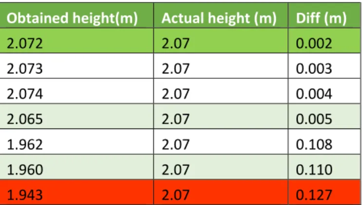
This section compares our obtained values with measurements from a total station which is a high accuracy instrument. Therefore, it is seen as fact.

Table 1 shows the actual measured height from the road to the markers and our obtained results. The values are randomly picked with some of the best and some of the worst results.

Obtained height(m)

Actual height (m) Diff (m)

2.072

2.07

0.002

2.073

2.07

0.003

2.074

2.07

0.004

2.065

2.07

0.005

1.962

2.07

0.108

1.960

2.07

0.110

1.943

2.07

0.127

Table 1, board height difference best to worst (assortment values with best and

worst difference).

Table 2 displays the obtained height from the road to each individual camera and compares the difference to documented values.

Camera Index Obtained height (m) Actual height (m) Diff (m)

2

6.692

6.676

0.016

4

6.750

6.676

0.075

0

6.813

6.675

0.138

1

6.855

6.676

0.179

3

6.862

6.676

0.186

5

6.878

6.676

0.202

Table 2, camera height difference. best to worst.

Table 3 shows the distance along the y-axis between the first camera and the second. Also, the first camera to the third.

Camera

Obtained distance (m) Actual distance (m) Diff (m)

3

3.991

3.776

-0.215

4

4.546

4.376

-0.170

Table 3, difference in position between reference camera 1 and 3. Also, difference

between ref. camera 1 and 4.

19

4.3 Reprojection error

OpenCV function solvePnP returns a reprojection error of 5.7 pixels (Table 4). It tells how well the algorithm could fit a rotation and translation to the pixel coordinates given. A reprojection error shows the spread of the points. It is retrieved in raw image pixels which is not the same as warped pixels. One warped pixel represents 3 cm. The raw image is distorted and has a perspective, which means the pixel size varies depending on where it is in the image. To get meaningful numbers, only reprojections errors from images close the image centre is

compared, where we measured that one pixel is approximately 0.97 cm. Also, worth noting, a small spread does not represent perfect accuracy, but a trustworthiness of the data.

Camera Image ID Reprojection error (pixels)

Reprojection error (cm)

0

54

5.019

4.856

1

57

4.248

4.110

2

53

4.645

4.495

3

51

5.745

5.559

4

55

3.866

3.741

5

53

5.444

5.268

Table 4, reprojection error worst case for all cameras.

4.4 Data visualized

A visualisation in matplot on mid-lane passage from each camera (Figure 10-13). Each camera has its own colour and a passage with each point representing the Aruco-board’s position. All positions are described in the new world coordinate system, which means that all exposures would ideally coincide into one line.

20

Figure 11, against driving direction view of data set (m).

21

Figure 13, side view of data set, displaying hight results for all exposures (m).

4.5 Real test

Our obtained camera rotation and position numbers was run in a real system to verify. In this system, all images are warped. The goal of the warp is to make the road identical in the camera pair, while objects closer to the camera should have perspective differences between the cameras. Correct rotations result in an ideal executed warp, where the road is identical between the camera pair. Figure 14 shows two images taken from the same camera pair at the same time. The reason there is black in the bottom left corner is that our origin was not identical with the origin in the real system.

22

5

Analysis

The detection rate of the Aruco-markers surpassed our expectations when considering how small the markers are relative the image plane. A 92% detection rate when ignoring the last three images in every camera proves that it is a reliable way of collection data points. It also shows that the markers should be enlarged for the future runs to ensure even better reliability. One marker covers approximately 0.05% of the total image plane. Considering how small that is, the detection rate is better than expected. This partly answers our research question, that it is possible to use Aruco markers with greater distances, such as 4 metres.

As seen in Figure 8, the marker corners were not detected with 100% accuracy, but within a margin of zero to three pixels. That is almost a ten-centimetre error. Enlarging the markers would generate more pixels for every marker, thus theoretically increasing the precision as the corners becomes bigger. If possible, ChArUco markers would be a better option. A normal Aruco marker only returns pixel coordinates of the four corners in every marker. This is where a chessboard pattern such as ChArUco shines as it contains a lot more line intersections than an Aruco-marker and can return more points. But it would have to be very large to be detected properly, which is a challenge in this environment as the space is limited. The disadvantage with a normal chessboard pattern is that OpenCV does not have a function for detecting multiple chessboards in one image. There are probably other libraries with this functionality, but Aruco has the advantage of being very flexible. They have a large dictionary of different markers available in different bit-resolutions. Every marker has its own ID, which is very convenient in a case where multiple calibration patterns must be visible in the same image. As the results tell, our tests had an accuracy error measured up to 21.5 centimetres. There are multiple factors involved. First, the marker corners are not detected within one pixel of error. Some exposures have an error of multiple pixels. On the other hand, the average height error is 13 centimetres. It is fair to say that the worst-case error represents a bad measurement or got enhanced by our math error which subtracts the rotations instead of multiplying. When tested in the real system we could verify that the method works even though it needs refinement.

Second, each camera has a vision of around 20 metres along the x-axis. With a distance between the markers in x of 2 metres, they only cover about 10% of the total image plane width. A bigger coverage would give more accurate x-axis representation. So, with only 10% coverage in x-axis, an error in y-axis affects the results more than if the distance were 50% of the whole image plane in x.

Third, subpixel accuracy is not implemented as of right now. This means the corner could be placed half a pixel wrong, or 1.5cm. As the board is double the height in width, the results are affected more if it is placed 1.5cm wrong in along the y-axis.

The motion blur of the vehicle is minor. It is clear by viewing the images, that the motion blur present was not the major factor to the performance hit regarding detection rate and pose estimation precision. A velocity speed of 80 km/h results in 2 pixels of motion blur. As mentioned in 4.3, two pixels are approximately 2 centimetres. This prevents the method from reaching to one-centimetre precision margin. However, in many road applications, driving slower or temporary stopping will be an option.

Finally, the method shows potential to be a viable calibration option for road applications. Although, it must be refined further with mentioned points above and in 6.4 first. Bigger markers and a bigger distance between markers are a must to minimize the worst-case errors.

23

6

Discussion and conclusions

6.1 Result

Aruco showed a detection rate of 71% with blurry images included and a 92% detection rate without.

Comparisons between measured positions done with a total station and our results were made. The worst-case error obtained was 21.5 centimetres.

Using the calculated position and rotation to obtain the reprojection error, the worst-case error was 5.7 pixels which approximately an error of 6 centimetres.

Matplot visualized the consistency between each exposure in one passage. Each passage created a straight line. Angles between the line were present where there should not be. This is due to the bug discussed in chapter 5 as well as 6.3.

Our numbers were run live on the system and showed reasonable results, which proves the bug did not have a substantial impact.

Viewing the images, the motion blur is minor. This was as expected, according to our calculations in section 1.4.

6.2 Implications

The results have shown that the method works and that there is a potential to reach a much higher precision than in our tests. As predicted the small marker size did affect the accuracy of the pose estimation as shown by the reprojection error table (Table 4).

Using a calibration pattern in a traffic surveillance application has shown to be feasible if the environment variables are correct. The possible distance from the camera to the markers correlates with how big the markers are. With the current marker size, the distance cannot be much larger than four to six without seriously affecting performance. The markers can also never be larger than the width of the driving lane which limits the height a camera can be placed on.

6.3 Limitations

It is worth noting, due to our failure in correctly calculating the difference between the reference camera and the other cameras, the results were compromised. This is visualized in 4.4. The angle difference is small between the cameras and that does help the results holding some ground truth. This only applies for the results where all cameras are described in the same coordinate system and not the reprojection errors as they are individual for each camera.

6.4 Conclusions and recommendations

As mentioned in 6.2, we can conclude that Aruco-markers on a moving vehicle works very well. To answer the research question, we conclude that the precision lands around a 20 centimetres error margin at worst. Having said that, considering all the improvements possible to the method such as larger markers, larger distance between markers and subpixel accuracy, the precision can be vastly improved. We also mentioned a user error from our part when subtracting and averaging the rotation vectors. It is hard to tell for sure how much it affected the results. Considering the rather small reprojection errors, which is not affected by our error as it is extracted from each exposure separately, we are confident it has not clouded the truth much.

A moving calibration pattern does introduce motion blur, which cannot be entirely removed unless there is no motion. A camera with high shutter speed is important if the vehicle is moving in higher velocities as in our tests.

24

6.5 Future work

If a continuation would be proceeded, the recording of the vehicle would have been done again with improvements mentioned above. The first step would be to correct our math errors. After that, the number one priority would be to make the markers bigger. It would make the corners better fit a pixel as well as increasing the detection rate and the precision of the calibration. The next step would be to widen the distance between the markers to cover a larger percentage of the image plane. Third, adding subpixel accuracy would further refine the method.

25

7

References

[1] Z. Zhang, M. Li, K. Huang and T. Tan, “Practical camera auto-calibration based on object appearance and motion for traffic scene visual surveillance,” in IEEE Conference on Computer Vision and Pattern Recognition, Anchorage, AK, USA, 2008 .

[2] N. Wang, H. Du, Y. Liu, Z. Tang and J.-N. Hwang, “Self-Calibration of Traffic Surveillance Cameras Based on Moving Vehicle Appearance and 3-D Vehicle Modeling,” in IEEE International Conference on Image processing, 2018.

[3] Z. P. Z. P. &. Y. W. Ruimin Ke, “Roadway surveillance video camera calibration using standard shipping container.,” International Smart Cities Conference (ISC2), p. 1–6. https://doi.org/10.1109/ISC2.2017.8090811, 2017.

[4] M. J. C. &. D. S. L. de Paula, “Automatic on-the-fly extrinsic camera calibration of onboard vehicular cameras.,” Expert Systems With Applications, pp. 41(4), 1997–2007. https://doi.org/10.1016/j.eswa.2013.08.096, 2014.

[5] F. Lv, T. Zhao and R. Nevatia, “Camera calibration from video of a walking human,” IEEE Transactions on Pattern Analysis and Machine Intelligence (Volume 28, Issue 9), pp. 1513-1518, 2006.

[6] S. Álvarez, D. F. Llorca and M. A. Sotelo, “Camera auto-calibration using zooming and zebra-crossing for traffic monitoring applications,” in 16th International IEEE Conference on Intelligent Transportation Systems, The Hague, Netherlands, 2013. [7] F. L. a. L. Z. Wang Qi, “Review on camera calibration,” 2010 Chinese Control and Decision

Conference, pp. pp. 3354-3358, 2010.

[8] Z. Zhang, “Flexible camera calibration by viewing a plane from unknown orientations,” Proceedings of the Seventh IEEE International Conference on Computer Vision, vol. vol. 1, no. vol.1, p. pp. 666–673, 1999.

[9] M. Hödlmoser, B. Micusik and M. Kampel, “Camera auto-calibration using pedestrians and zebra-crossings,” in IEEE International Conference on Computer Vision Workshops (ICCV Workshops), Barcelona, Spain, 2011.

[10

] N. K. Kanhere and S. T. Birchfield, “A Taxonomy and Analysis of Camera Calibration Methods for Traffic Monitoring Applications,” IEEE Transactions on Intelligent Transportation Systems ( Volume: 11 , Issue: 2), pp. 441-452, 2010.

[11] B. &. T. V. Caprile, “Using vanishing points for camera calibration.,” International Journal of Computer Vision, no. 4(2), p. 127–139, 1990.

[12

] OpenCV, https://docs.opencv.org/3.4/df/d4a/tutorial_charuco_detection.html. [Accessed 25 10 “docs opencv,” 25 10 2020. [Online]. Available: 2020].

[13

] S. S. H. T. K. M. D. I. M. &. K. A. Miyata, “Extrinsic Camera Calibration Without Visible Corresponding Points Using Omnidirectional Cameras,” IEEE Transactions on Circuits

and Systems for Video Technology, 28(9), 2210–2219.

https://doi.org/10.1109/TCSVT.2017.2731792, 2018. [14

]

Z. Zhang, “A flexible new technique for camera calibration,” in IEEE Transactions on Pattern Analysis and Machine Intelligence, vol. 22, no. 11, pp. pp. 1330-1334, Nov. 2000. [15

] R. M.-S. F. .. M.-C. a. M. .. M.-J. S. Garrido-Jurado, “Automatic generation and detection of highly reliable fiducial markers under occlusion,” Pattern recognition, vol. vol. 47, no. no. 6, p. pp. 2280–2292, 2014.

[16

] R. M.-S. a. R. M.-C. F. J. Romero-Ramirez, “Speeded up detection of squared fiducial markers,” Image and vision computing, vol. vol. 76, pp. pp. 38–47, 2018, 2018. [17

] R. M.-S. F. .. M.-C. a. R. M.-C. S. Garrido-Jurado, “Generation of fiducial marker dictionaries using Mixed Integer Linear Programming,” Pattern recognition, vol. vol. 51, p. pp. 481–491, 2016.

[18

] OpenCV, https://docs.opencv.org/3.4/d9/d6a/group__aruco.html#ga13a2742381c0a48e146d23“OpenCV docs,” OpenCV, 28 08 2020. [Online]. Available: 0a8cda2e66. [Accessed 28 08 2020].

26 [19

] “Camera Calibration and 3D Reconstruction,” 31 12 2019. [Online]. Available: https://docs.opencv.org/2.4/modules/calib3d/doc/camera_calibration_and_3d_recon struction.html. [Accessed 17 2 2020].

[20

] K. Levenberg, “A method for the solution of certain non-linear problems in least squares,” Quarterly of Applied mathematics, vol. 2, pp. 164-168, 1944. [21

] X.-S. Gao, X.-R. Hou, J. Tang and H.-F. Cheng, “Complete solution classification for the perspective-three-point problem,” IEEE Transactions on pattern Analysis and machine Intelligence, vol. 25, pp. 930-943, 2003.

[22

] R. C. Bolles and M. A. Fischler, “Random sample consensus: a paradigm for model fitting with applications to image analysis and automated cartography,” Communications of the ACM, vol. 24, no. 6, 1981.

27

8

Appendix