Does Large-Scale Gold Mining Reduce Agricultural Growth? Case studies from Burkina Faso, Ghana, Mali and Tanzania

Does Large-Scale Gold Mining Reduce Agricultural Growth?

Case studies from Burkina Faso, Ghana, Mali and Tanzania

Magnus Andersson1, Ola Hall2, Niklas Olén3, and Anja Tolonen4

Abstract

We apply a novel analytical framework based on medium resolution satellite data for the period 2001 – 2012 to estimate the effects of gold mining on agricultural production in Ghana, Mali, Tanzania and Burkina Faso. Our analysis finds a strong correlation between official statistics of agricultural production and vegetation index from satellite data at district level in these countries. Agricultural productivity as proxied by greenness index (NDVI) does not decrease in the proximity of large scale gold mines. Our empirical estimations show that economic activity as proxied by night lights, increase in the proximity of mining but the estimates remains statistically insignificant.

1 _{Department of Urban Studies, Malmö University, magnus.e.andersson@mah.se} 2 _{Department of Human and Economic Geography, Lund University}

3 _{Department of Physical Geography and Ecosystems Analysis, Lund University} 4 _{Department of Economics, University of Gothenburg}

1

1. Introduction

The aim of this paper is to gain a better understanding of the impact of resource extraction on local economic growth, with a special focus on agricultural growth. The issue of interest is whether the opening of mines has spillover effects on the local economy and especially on the agricultural sector. Agricultural production could be affected by mining activities in several ways. Mining could lead to a rise in local wages, reduce profit margins in agriculture and lead to exit of many families from farming – something akin to a localized Dutch disease problem. Negative environmental spillovers such as pollution or local health problems could also dampen productivity of the land and of the farmers, and thereby reduce the viability of farming. Alternatively, mining could create a mini-boom in the local economy through higher employment and higher wages that can lead to an increase in local area aggregate demand, including for regional food crops.

This paper uses remote sensing data to estimate levels and changes in agricultural and non-agricultural production in mining and non-mining localities in Burkina Faso, Ghana, Mali and Tanzania. The study investigates the spatial relationship between mining activities and local agricultural development by using a vegetation index as a proxy for agricultural production. In order to estimate the level and composition of production – agricultural and non-agricultural – at the local level the paper selects a radius around the mining areas. For all the three countries, 32 mines were identified.

Satellite remote sensing missions are generally designed for specific applications, often earth sciences related, such as vegetation classification and weather forecasting. Very few, if any, sensors are designed for social science applications (Hall, 2010). The DMSP-OLS sensor, also known as “nighttime lights”, has attracted recent attention due to its capability to depict human settlement and development. It is sensitive enough to detect street lights and even fishing vessels at sea (Sei-Ichi, Fukaya, Saitoh, and Semedi, 2010). The light detected by the DMSP-OLS is largely the result of human activities, emitted from settlements, shipping fleets, gas flaring or fires from swidden (slash and burn) agriculture. Therefore, nighttime light imagery serves as a unique view of the earth’s surface which highlights human activities. One of the central uses of the nighttime lights dataset is as a measure of and proxy for economic activity. The relationship between economic activity and light has been explored by several authors and all have concluded that there is indeed a positive relationship between the light emitted and the level of economic development within a region. This understanding has been used to estimate both GDP and economic growth. This paper is a contribution to the literature on the connection between extractive industries and local clustering of economic activity using remote sensing data.

The rest of the paper proceeds as follows. Section 2 reviews the literature on remote sensing and economic activities with particular focus on agriculture. Section 3 describes the data used in the study. Section 4 describes the various methodologies and their results including the econometric results using a difference-in-difference estimation framework (previously employed to understand the economic effects of gold mining in Africa by Aragón and Rud (2013), Tolonen (2015), and Kotsadam et al., (2015). Section 6 concludes the paper.

2. Remote sensing and economic activities

Nightlight and economic activities

Some recent economic studies have exploited human generated night-time light data to understand the structure, growth and spatial distribution of economic activities in countries or localized areas (Elvidge et al., 1997; Sutton and Costanza, 2002; Doll, Muller and Morley, 2006; Ghosh et al, 2010; Henderson, Storeygard and Weil, 2012; Ebener et al., 2005, Chen and Nordhaus, 2011). An early identification of the strength of the relationship between nighttime lights and economic development was made by Elvidge, et al. (1997), who explored the relationship between lighted area and GDP, population and electrical power consumption in the countries of South America, the United States, Madagascar and several island nations of the Caribbean and the Indian Ocean. Using simple linear regression over a single year (1994/1995) they found that GDP exhibits a strong linear relationship with the lighted area.

Elvidge, et al.’s (1997) study is unique in that it associated the relationship between economic activity and lighted area. Most other publications using such data related economic activity with light intensity. Doll, Muller and Morley (2006) were one of the first to apply this relationship to estimating economic activity on a national and sub-national basis. They identified a unique linear relationship between gross regional product (GRP) and lighting for the European Union and the United States using 1996/1997 data and found that one linear relationship was not appropriate since some cities were outliers. However, once the outliers were removed, they were able to generate simple linear regressions – which showed strong links between GRP and light intensity - for each country, which they used to generate a gridded map of GRP at the five kilometer level. Building on this approach, Ghosh et al. (2010) use gross state product (GSP), GDP and light intensity in 2006 for various administrative units in the states of China, India, Mexico and the United States to obtain an estimate of total economic activity for each administrative unit. These values were then spatially distributed within a global grid using the percent contribution of agriculture towards GDP, a population grid and the nighttime lights image. This is an improvement over Doll, Muller and Morley (2006) in the sense that it was able to assign economic activity to agricultural areas, which are not usually picked up by the nighttime lights dataset since they are not often lit. This is an important observation about night light data that will inform our study.

Chen and Nordhaus (2011) were one of the first studies to exploit time series variation in GDP and night light. To show the strength of the correlation between economic activity and night light, their method assigns weights to light intensity in order to reduce the difference between the true GDP values and the estimated GDP (that is, they minimize mean squared error) for all countries of the world for the period 1992 to 2008. They show that while light intensity data does not add much value – that is, does not provide any additional information than actual data – to data rich countries, the opposite is true for data poor countries. They show that GDP estimation in

data-poor countries, both at the national and sub-national level, improves substantially with night light data.

One of the most recent applications of the nighttime lights dataset in relation to economic activity is by Henderson, Storeygard and Weil (2012). Rather than exploring the relationship of lights with GDP levels, they look at the relationship with GDP growth. Like Chen and Nordhaus (2011), they use a time series of growth and light data for the period between 1992 and 2008. Their statistical model correlates GDP growth using country specific economic data with light intensity values. Similar to Chen and Nordhaus (2011), they construct different weights for the light data and existing economic data based on the quality of the economic data. They found that for countries with “bad” data, there are often large differences (both positive and negative) between the recorded economic growth and the estimated growth.

In general, this short review of the literature using remote sensing data leads to two conclusions. First, it demonstrates that such data provide a strong and accurate prediction of economic activity. Second, although various types of remote sensing data are available, the one that is most widely used tend to be night light data. To date most of the studies have used light intensity, rather than lighted area, to explain either GDP or its growth within and across countries in a given year and, on a few occasions, over time. However, night light, while certainly informative of human activity, does not exhaust economic activity in all places. In particular, in countries where electricity is unreliable and there is significant reliance of generators for production activities, night light could be underestimating economic activity. This would be true especially, if the generators are turned on at all at night for cost reasons. In addition, in countries that are mostly rural and where the mainstay of the economy is agriculture, an over reliance on night light might miss a big fraction of economic activity, even if electricity in fact reliable. Fortunately, remote sensing data can be used for capturing agricultural activities as well, and the next section discusses one such data.

NDVI and agricultural production

Numerous methods exist for estimating productivity of the agricultural sector with remote sensing technology. But most approaches rely on the idea that vegetation, including crops, is very reflective in the red and near-infrared (NIR) wavelengths. Combinations of these two wavelengths (i.e. vegetation indices) are good measures of plant vigor and are the mainstay of nearly all approaches to crop yield estimation (Lobell, 2013). Yields are then estimated through establishing the empirical relationship between ground-based yield measures and some vegetation indices, typically Normalized Difference Vegetation Index (NDVI).

Errors in remote- sensing crop- yield estimates vary mainly as a function of sensor properties (spatial-, temporal-, and spectral resolution) and landscape complexity. Classification of crop types is more problematic in regions characterized by multiple crops with similar life cycles (that is, phonologies), or in regions with intercropped fields (Lobell, 2013). Additional complexity is added with cassava, a major crop for which even farmers themselves have difficulties in estimating yields. This is basically because it is a root crop with staggered harvesting, but also

with widely differing above-ground architecture. Sometimes overlooked is the problem of cloud cover in satellite based remote sensing which could severely limit the number of available observations for a particular geographic region. Nevertheless, yield estimation in mixed cropping systems, characteristic of African smallholder agriculture, should be possible, using a remote sensor platform with the correct properties. This indeed is the case and in the next section we describe the data we use to obtain local economic production, including agriculture.

3. Data

We use three sources of remote sensing data to estimates the effects of mining on local economic activity: nighttime lights, NDVI, and forest loss. Nighttime lights data is from the National Oceanic and Atmospheric Association’s National Geophysical Data Center (NOAA-NGDC). The NOAA-NGDC produces three annual nighttime lights products. They are the cloud-free, average visible lights and stable lights composites5. This data was processed in two steps: first, gas-flares were removed using a set of ESRI shapefiles available from NOAA-NGDC which contain polygons outlining the location of gas flares for each country. Second the data was inter-calibrated to allow cross-year analysis. The inter-calibration procedure developed by Elvidge et al. (2009b) was aimed at overcoming the limited comparability of the DMSP-OLS data by calibrating each composite against one base composite. It is a regression based technique that works under the assumption that the lighting levels in a reference area have remained relatively constant over time and can therefore be used as the dependent variable.

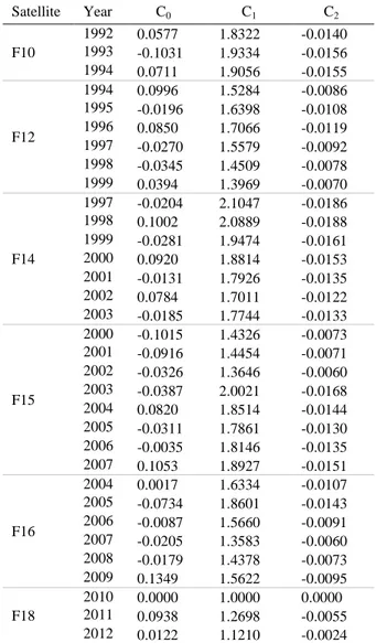
Table 1 shows the satellite-year pairs that are used for the inter-calibration. As indicated in the Table, satellite F10, and year 2010 (denoted as F182010) was chosen as the base composite because, overall, its pixels contained the highest intensity, measured by digital numbers (DN)6. Next, for each composite we run a regression that is quadratic in its original values, as shown below.

𝑦𝑦 = 𝐶𝐶0+ 𝐶𝐶1𝑥𝑥 + 𝐶𝐶2𝑥𝑥2

Table 1 shows the resulting calibration coefficients, which were applied to each composite so that a new value (y) was calculated based on the original value (x). Any values over 63 were truncated so that the range of the values remained between 0 and 63. In principle, we can obtain light intensity data for very small areas, up to a cell size of 1 km2. Alternatively, one can take the average over small areas and create twenty-one composites each representing one year of nighttime lights between 1992 and 2012.

5 _{See NOAA-NGDC, 2014b for a description of each of these datasets}

6 _{In their study, Elvidge et al. (2013; 2009b) selected F121999 as the base composite. The difference in the selection}

is attributed to the fact that Elvidge et al. (2013; 2009b) were inter-calibrating a world-wide dataset while the present study examines only the African case.

5

Table 1. Inter-calibration coefficients. Satellite Year C0 C1 C2 F10 1992 0.0577 1.8322 -0.0140 1993 -0.1031 1.9334 -0.0156 1994 0.0711 1.9056 -0.0155 F12 1994 0.0996 1.5284 -0.0086 1995 -0.0196 1.6398 -0.0108 1996 0.0850 1.7066 -0.0119 1997 -0.0270 1.5579 -0.0092 1998 -0.0345 1.4509 -0.0078 1999 0.0394 1.3969 -0.0070 F14 1997 -0.0204 2.1047 -0.0186 1998 0.1002 2.0889 -0.0188 1999 -0.0281 1.9474 -0.0161 2000 0.0920 1.8814 -0.0153 2001 -0.0131 1.7926 -0.0135 2002 0.0784 1.7011 -0.0122 2003 -0.0185 1.7744 -0.0133 F15 2000 -0.1015 1.4326 -0.0073 2001 -0.0916 1.4454 -0.0071 2002 -0.0326 1.3646 -0.0060 2003 -0.0387 2.0021 -0.0168 2004 0.0820 1.8514 -0.0144 2005 -0.0311 1.7861 -0.0130 2006 -0.0035 1.8146 -0.0135 2007 0.1053 1.8927 -0.0151 F16 2004 0.0017 1.6334 -0.0107 2005 -0.0734 1.8601 -0.0143 2006 -0.0087 1.5660 -0.0091 2007 -0.0205 1.3583 -0.0060 2008 -0.0179 1.4378 -0.0073 2009 0.1349 1.5622 -0.0095 F18 2010 0.0000 1.0000 0.0000 2011 0.0938 1.2698 -0.0055 2012 0.0122 1.1210 -0.0024

For our purpose, since we are interested in assessing the impact of mining on local economic activity, we create a sum of light (SOL), a measure of the total intensity of lighting, for all the cells around the mining areas and for each unit of the highest administrative level possible in each country. The latter serves the purpose of helping us link the intensity of light to local economic activity, where unlike the areas around the mine, the local here is defined as district. The NDVI7 data is provided as a global dataset with a 16 day temporal resolution and a spatial resolution of 250m. NDVI is a dimensionless spectral index that relates to the photosynthetic uptake by vegetation (Myneni and Williams, 1994; Sellers, 1985). It is calculated from the near infrared (NIR) and red wavelength bands by using the following relationship:

7

The NDVI from Moderate Imaging Spectro-radiometer (MODIS) vegetation indices product MOD13Q1 were used (ORNL DAAC, 2011).

6

NDVI = (NIR – Red) / (NIR + Red)

It has previously been shown that NDVI is related to, for example, the vegetation greenness, leaf area index (LAI), and primary productivity of the vegetation (Johnson, 2003; Paruelo et al., 1997). Furthermore, it has been documented that a time series of NDVI can be used to assess the changes in vegetation cover and responses over time (Hill and Donald, 2003). Additionally, it can be used to estimate agricultural yields (Labus et al., 2010; Ren et al., 2008). This makes it possible to evaluate the vegetation status and the agricultural productivity on a large scale, by using remotely sensed NDVI, in regions where field data are sparse.

A mask was constructed to exclude land covers that are not part of the agricultural economy8. The mask was produced by using 2005 land covers as a mask. The primary land cover scheme identifies 17 land cover classes9, which includes 11 natural vegetation classes, 3 developed and mosaicked land classes, and three non-vegetated land classes. Here, desired classes were Croplands (Number 12) and Cropland/Natural vegetation mosaic (Number 14). For classification numbers 12 and 14,yearly amplitude NDVI data on pixel level using mean production at district level.

The recent global dataset10 of Hansen et al (2013) was used to quantify forest loss annually. This is a map of the extent, loss and gain of global tree cover for the period from 2000 to 2012 at a spatial resolution of 30m. The dataset improves on existing knowledge of global forest extent and change by being spatially explicit, quantifying gross forest loss and gain, providing annual loss information and quantifying trends in forest loss. Forest loss was defined as a stand-replacement disturbance or the complete removal of tree cover canopy at the Landsat pixel scale. Tiles were merged into larger composites and reclassified into twelve layers, one for each year, thus separating each individual forest loss year. Instead of SOL, sum of forest loss was calculated in the same way as night lights.

We also obtained agricultural production data from the statistical offices in Ghana, Tanzania and Mali to analyze the relationship between NDVI and agricultural production. The data was compiled at the district level and represent all agricultural products produced during one year. Ghana had data for year 2001 to 2012, Tanzania for year 2007 and 2008 and Mali 2002 to 2007. Finally, official GDP data were also obtained from the World Bank World Development Indicators open data database (The World Bank Group, 2014). Data were downloaded for each country on a yearly basis from 1992 to 2012. The official GDP data represents the value of the gross output produced in a country minus the value of intermediate goods and services consumed in production. All GDP data are expressed in constant 2005 US dollars (USD).

8

For this purpose, the MODIS Land Cover Type product (MCD12Q1) was used (Friedl et al., 2010).

9

These are the land cover classes defined by the International Geosphere Biosphere Programme (IGBP)

10

Annual forest loss data was downloaded from http://www.earthenginepartners.appspot.com/science-2013-global-forest/download.html

7

4. Growth Model and Results

In order to use these remote sensing data, we have to demonstrate that they can indeed predict or track the pattern of data collected through statistical offices. In other words, we have to demonstrate the strength of the correlation between the remote sensing data and the actual data that is collected by administrative agencies in countries. Especially, for NDVI we need to have some knowledge of the agricultural production at district levels, at least, and preferably at even more local administrative units. In this spirit, this section has 3 parts. First, it will establish the correlation between NDVI and actual agricultural production. Part 2 estimates the national and local growth model based on time series analysis covering the period of 2001 to 2012 at district level in the case countries. The purpose of this part is to combine nightlight, NDVI and forest loss data to estimate the size of the local economy. Part 3 then uses such a model in a difference-in-difference framework to provide an estimate of the effect of mining on local economic activity, with particular attention on local agricultural production.

A. NDVI and agricultural production

The remote sensing data allows us to compute NDVI for areas of any size. However, we have actual agricultural production only at the district level. Therefore, our first task is to show a spatial correlation of NDVI and actual agricultural production at districts levels. An important difference between spatial and traditional (a-spatial) estimations, such as OLS regression, is that spatial statistics integrate space and spatial relationships directly into their models. Depending on the specific technique, spatial dependency can enter the regression model as relationships between the independent variables and the outcome variable, between the outcome variables and a spatial lag of itself, or in the unexplained (that is, error) terms. Geographically weighted regression (GWR) is a spatial regression, applied at the small geographic areas, that generates parameters disaggregated by the spatial units of analysis. This allows for the assessment of the spatial heterogeneity in the estimated relationships between the independent and dependent variables (Fotheringham et. al., 2002). We find a strong association between actual production of agricultural products and NDVI using spatial regression.

Figure 1 illustrates the varying spatial relationship between our two estimates of agricultural production - NDVI and official statistics covering agricultural production. The Figure demonstrates using the NDVI values and agricultural production using 2007 for illustration. Other years show similar results and the summary of the strength of the association is shown in the Annex (see Figure 3 and Table 1 in Appendix). The sum of NDVI at the district level is used as a predictor for the level of agricultural production. The pattern that emerges is one of a highly- to moderately-strong correlation between agricultural production and NDVI in areas with high population densities. In most years and countries – with the exception of Mali - over 60 percent of the variation in district level agricultural production can be explained by the differences in the average district level NDVI intensity (see Table 1 in Annex). We are not able to determine if the agricultural data includes non-marketed production, which in all these countries could be

substantial. That said, the strong correlation between NDVI and agricultural production gives us confidence to use NDVI to predict agricultural production for small areas – say around the mine.

Fig. 1. GWR Dependent variable Total agricultural production by district and Independent variable, sum

of NDVI Intensity, by district (2007)

B. National Growth Model

In addition to its impact on agriculture, we are interested to know whether mining has substantial economic benefits – spillover effects – on local economies. The previous section showed that the strong association between NDVI and agricultural production justifies our use of the NDVI data for measuring the changes to agricultural production around the mines. Similarly, we could use the night light data, which has been demonstrated to predict economic activity, to capture changes to the local economy around the mines. Unlike agriculture, we do not have district level GDP, so we would have to first estimate a national model and then use the parameters from such a model to obtain local economic production.

The basic estimation strategy follows Henderson et al. (2012), whose framework can be shown as:

γ

= ψ�x

+ c

+ d

+ e

(1)

where 𝛾𝛾_{𝑗𝑗𝑗𝑗} is the true GDP of country j in time t. 𝑥𝑥_{𝑗𝑗𝑗𝑗} is the level of observed nighttime light at corresponding country and time. 𝑐𝑐_𝑗𝑗, 𝑑𝑑_𝑗𝑗, stand for country and year fixed effects and 𝑒𝑒_{𝑗𝑗𝑗𝑗} stands error term. As stated above, this is a model of the aggregate economy. It suggests that the total production or total economic activity (or its changes) is explained by level of measured night light (or its percentage growth) observed by satellite adjusted for some country and time-invariant effects and an error term.

As is the tradition, the error term is assumed to be uncorrelated with GDP measurement, and in this case, given the GDP and the night light come from two independent sources, that would seem to be true. However, using gridded data of land cover and night-time light, we have found that it is possible for agriculture’s value-added to increase without emitting more observable night-time light into space. If this is the case, then the error term is actually dependent on the agricultural share as the higher the agricultural share the higher the measurement error from the night time lights.

Given this observation, our estimation follows the framework in equation (1), but take note of the fact that not all economic growth, especially in heavily agricultural societies, is captured by growth in observed night-time light only. Our working assumption is that night-time light observed in space is the result of growth in only the non-agricultural sector. We therefore split Henderson et al. (2012) model into a separate non-agricultural (eq. 2) and agricultural (eq. 3) parts, which are then combined as in (eq. 4).

γ_jtna = ψ�nax_jtna+ c_jna+ d_tna+ e_jtna (2) γjta = (ψ�a1 ψ�a2 … ψ�an) ⎝ ⎜ ⎛ljt a1 ljta2 ⋮ ljtan_⎠ ⎟ ⎞ + cja+ dta+ ejta (3)

Equation (2) is the familiar model that links GDP level (or growth) to the sum (or growth) of night time lights. We argue here that this model is mostly predictive of non-agricultural data. In equation (3) we extend this model to agricultural sector by introducing the categorical variable, land cover, using MODIS NDVI and forest loss. Finally, we obtain 3 models of income (growth)

for each country which combines nightlight, NDVI, and forest loss, as can be seen in equations 4-6.

We are designing the model so the regression line departs from the origin with a y-intercept being equal to 0. The rationale behind not using the intercept is that we in the second step of the model are estimating local growth by using the national growth model to fit with local parameters on district level. The dynamics of the local economy is dependent on the relationship between the variables used in the national growth model. Including a national intercept term would then have a mismatch due to the spatial scale of the local estimations.

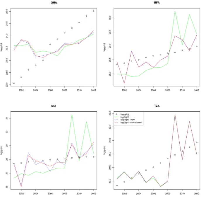
Figure 2 shows the correspondence between the actual evolution of aggregate production and the pattern of predicted output that can be obtained using the 3 different models (4-6) for each country.

Log GDP ~ Log Nightlight (4)

Log GDP ~ Log Nightlight + NDVI (5)

Log GDP ~ Log Nightlight + NDVI + Forestloss (6)

Fig. 2. Actual and Predicted log (GDP) using 3 different models (2001-2012).

There are three observations that one can draw from Figure 2 (details about the bivariate between log (GDP) and the three predictors can be seen in Appendix). First, the remote sensing data are highly predictive of the actual evolution of GDP in all countries and with better predicted levels of GDP when including all three types of remote sensing data. The best fit are models for Mali and Burkina Faso where actual log (GDP) and predicted log (GDP) using (log night light, forest loss and NDVI) are very close for almost every year. By contrast, for Tanzania and Ghana, while the correlations are strong, there are periods when the remote sensing data overestimates and others when it under predicts the total production in the two countries. In Ghana, remote sensing

data tends to predict lower overall output through most of the period, while in Tanazania, the remote sensing data predicts a log (GDP) that was higher than reported after 2009 and lower prior to that period.

Second, as we suspected, night light alone is not sufficient to predict aggregate production. While it is true that night light stands out as highly correlated with GDP, inclusion of the NDVI improves the fit of the model (Table 2). In fact the country models seem to suggest that night lights with NDVI performs better than any other specification (e.g. night lights, NDVI and forest loss) in predicting log (GDP). In no country are NDVI and forest loss statistically significant jointly. As a result, we drop the forest loss variable in all our models.

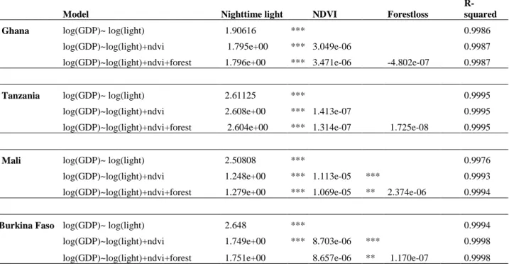
Table 2: Multiple linear regression coefficients for growth model specified in equation 4.

Model Nighttime light NDVI Forestloss R-squared Ghana log(GDP)~ log(light) 1.90616 *** 0.9986

log(GDP)~log(light)+ndvi 1.795e+00 *** 3.049e-06 0.9987

log(GDP)~log(light)+ndvi+forest 1.796e+00 *** 3.471e-06 -4.802e-07 0.9987

Tanzania log(GDP)~ log(light) 2.61125 *** 0.9995

log(GDP)~log(light)+ndvi 2.608e+00 *** 1.413e-07 0.9995

log(GDP)~log(light)+ndvi+forest 2.604e+00 *** 1.314e-07 1.725e-08 0.9995

Mali log(GDP)~ log(light) 2.50808 *** 0.9976 log(GDP)~log(light)+ndvi 1.248e+00 *** 1.113e-05 *** 0.9993

log(GDP)~log(light)+ndvi+forest 1.279e+00 *** 1.069e-05 ** 2.374e-06 0.9994

Burkina Faso log(GDP)~ log(light) 2.648 *** 0.9994 log(GDP)~log(light)+ndvi 1.749e+00 *** 8.703e-06 *** 0.9998 log(GDP)~log(light)+ndvi+forest 1.751e+00 8.657e-06 ** 1.170e-07 0.9998 Notes: Significance codes 0 ‘***’ 0.001 ‘**’ 0.01 ‘*’ 0.05 ‘.’ 0.1 ‘ ’ 1

Third, even though agriculture accounts for the largest share of economic activity in all these countries, NDVI is strongly significant only for model of Burkina Faso and Mali. Adding forest loss to the model does not change the model fit and the variable is not significant in any of the countries.

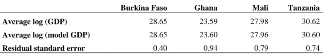
Table 3: Standard error of residuals between model and observed together with average of observed and

modeled GDP.

Burkina Faso Ghana Mali Tanzania Average log (GDP) 28.65 23.59 27.98 30.62

Average log (model GDP) 28.65 23.60 27.96 30.60

Residual standard error 0.40 0.94 0.79 0.74

Growth model at district levels

Ideally we would like to estimate a model linking GDP at local level to geo referenced data. Unfortunately, while the geo referenced data can be compiled for areas smaller than even a district, none of our four case studies collect GDP at the district level. Therefore, we use the parameters of the relationship between GDP and geo referenced data at the national for each country to impute local district level production in each country. The models are based on the regression results from equation (4-6) and presented in Table 3. The local growth model is based on the national growth model.

When developing the growth model for districts several methods where used in order to provide an accurate local dimension of the local economy. Population data and average household expenditure on district levels were included as weights in the model estimating local growth patterns. However, population on district level was highly correlated with nightlight intensity on district levels and average household expenditure on district levels was highly correlated with GDP on local levels (for details on the correlation analysis see Appendix) and therefore not used in the estimations.

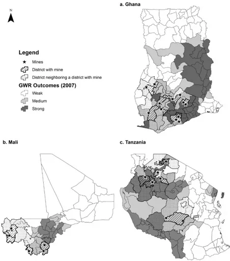
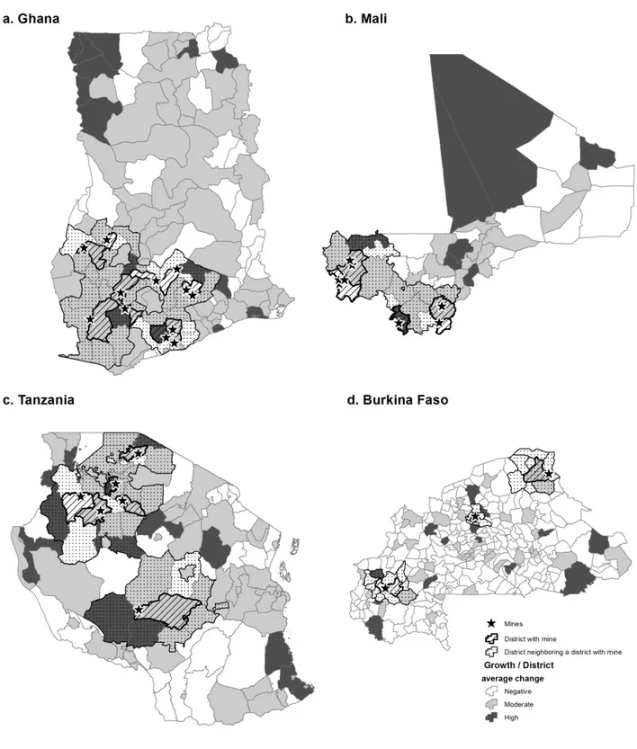
The results of the district level growth patterns are displayed in a series of maps and graphs (see Figure 3 in the Appendix). Figure 3 is a map of the imputed growth patterns at the district level. It tags districts into those that are predicted to have had negative, moderate or high growth. These maps provide a visual display of the geography of growth in each country.

A look at the map leads three main conclusions. First, average growth in mining districts appears to be higher than non-mining districts. In Ghana, the average growth rates turn positive if the growth in districts neighboring the mining districts area taken into account. The map suggests that effects on mining could evolve differently around mining and non-mining areas in different countries. And the differential evolution could have an impact on local economic growth. However, to test whether these spatial patterns of measured local economic growth are due to mining activities requires a more rigorous test than just a visual inspection. We turn to discuss such a test and the results in the next section.

C. Night Lights and NDVI in a Difference-in-Difference Framework Empirical Framework

To understand if night lights and greenness index in mining communities with the onset of mining, we employ an empirical estimation strategy called difference-in-difference (previously employed to understand the economic effects of gold mining in Africa by Aragón and Rud (2013), Tolonen (2015), and Kotsadam et al., (2015). This strategy allows us to compare outcomes in the geographic proximity of mines, with areas further away, both before and after the mines start producing. In effect, we are making three comparisons: close to far away, as well as before and after, and both comparisons at the same time. We can model the cross-sectional differences in areas with an active mine, and without active mines:

Yjt = β1activejt+ εj

Where Y is the outcome variable (night lights and NDVI), active is a binary variable that takes value 1 if the mine is active in that year, and subscript j is for the mine, and t for the year. We can also model the importance of proximity:

Yj= β1closej+ εj

Where close captures the cross-sectional difference between areas that are close to mines and those that are further away. What we are interested in knowing, however, is the relative change that happens in the geographic proximity of mines with the onset of the mine, compared to what happens far away from the mine. We capture this with the difference-in-difference estimation model which includes an interaction effect of the two binary variables:

Yjt= β1activejt+ β2closej+ β3activejt∗ closej+ δj+ εjt

Where δ_j is a mine fixed effect, which means that we account for any change that is peculiar to a mine. We can also use year fixed effects, which will take care of year-specific shocks that happens across all mines. To decide the relevant distances, we rely on Aragón and Rud (2013), Tolonen (2015), and Kotsadam et al., (2015), who show that areas at up to 20km radius are relevant to use to understand the footprint of gold mines in Africa. Moreover, we rely on the geographic results found in this paper. We chose a distance of 20km to understand the footprint close to mines (10km is not possible because of lack of quality spatial data at this resolution). We

compare with an area which is 50 to 100km away because the same literature suggests that beyond 50km, the mines have little economic footprint. This makes areas further than 50 km as suitable comparison group.

Results

Graph 1 explores the change in the two groups, close and far away, over the mines’ lifetime. On the horizontal axis is the mine year, counting from 4 years before mine opening, highlighted by the red vertical line, to four years after mine opening. The graphs are based on summary statistics, and we do not control for any systematic differences across the mines included here. Overall, it seems like areas very close to mines are on a steeper trend in night lights than are areas further away, especially as we get closer to the mine opening year which is highlighted by the red vertical line. One interpretation of this pattern is that from a few years before the mine starts extracting gold, economic activity increases in these areas. A reason why this happens before the actual mine opening year is because mines are capital intensive and the local economy is stimulated during this investment phase, a pattern confirmed in previously mentioned econometric studies.

For NDVI we do not see a big difference across the areas. Although both areas seem to be on an upward sloping trend, this needs to be interpreted with caution, because it can be driven by the unbalanced sample.

Graph 2, 3, and 4, show the same summary statistics but for each individual mine. For night lights, there is a divergence for most mines in the sample as we get close to the mine opening year, and a convergence after a few years in some of the cases (Ahafo, Chirano and North Mara). We have less data points for NDVI and we discern almost no changes across the areas, (Graph 4). If anything, we detect that areas close to mines are getting relatively greener over time, compared with areas further away.

Graph 1: Night Light, NDVI over Mine Lifetime

Graph 2: Night Light by Mine

Graph 3

NDVI by Mine

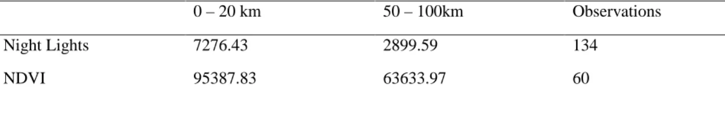
Table 4 shows the mean values of areas close to mines and those far away from mines, but not taking into account the time-variation in mining activities. Mining areas have higher night light score, and are greener on average, compared to areas that are 50 to 100km further away.

Table 4

Mean values in Night lights, NDVI

0 – 20 km 50 – 100km Observations

Night Lights 7276.43 2899.59 134

NDVI 95387.83 63633.97 60

Notes: Summary statistics (mean) value for the three outcome variables across the treatment and control group, in the

cross-section.

Table 5 shows the regression results from the strategies outlined in the Empirical Framework section. Areas close to active mines have higher level of lights at night (Column 1, Panel A). But so do areas that are simply close (Column 2) to a mine (active or not), although in this case the estimates are not statistically significant. But a parameter of interest is the interaction effect (Columns 3 and Column 4, Panel A), which conveys the idea of the measured change in economic activity - proxied by night lights - in areas that are close to active mines11. The estimated effect is positive, although this impact is not precisely estimated since it is not statistically significant. Controlling for time fixed effects increases the size of the impact but does not improve the statistical significance.

One reason for the imprecise measure could be related to the small sample size. There are only a few mines in each of these countries that can be used in the estimation. There is also the possibility that we may be overestimating the effect size because we may not capture changes in the composition of local production with just night lights. For instance, if households engaging in subsistence farming did not have electricity, but demand more of it in order to change to more modern sectors at the time of opening of the mine, then the increased demand for electricity will lead to an increase in night lights. However, the decrease in farming that will result from occupational switching will not be reflected in the changes in night light if subsistence farming does not use electricity. In such a scenario, we would be overestimating the effect of the mine on the local economy. However, Kotsadam et al. (2015) estimate that non-migrant households that live close to gold mines in Ghana have better access to electricity, which suggests that any increase in electricity is because of the onset of the mine. Therefore, we take the positive effect, albeit statistically insignificant, as suggestive evidence that gold mining spurs local economic

11 _{According to the visual evidence presented in Graph 1, where the local economy is spurred roughly 2 years}

before mine opening, we drop the years immediately preceding the mine opening from the regression in a robustness check. The results are slightly larger for the interaction term, as expected, but remain insignificant. The results from this exercise are available upon demand.

18

growth, and is in line with evidence showing that gold mining can bring local structural change by generating non-farm employment (Kotsadam et al., 2015; Tolonen, 2015).

Note however, that if households engaging in subsistence farming do not have, and need, electricity access change to more modern sectors which demand electricity at mine opening, this will cause an increase in night lights. In such a scenario, we may overestimate the effect of the mine on the local economy since the decrease in farming is not associated with any change in night lights, if it was not reliant on electricity for power. However, Kotsadam et al., (2015) estimate that non-migrant households that live close to gold mines in Ghana have better access to electricity, which is in line with this finding.

Table 5

Cross-sectional and time variation in Night lights and NDVI

(1) (2) (3) (4)

VARIABLES Active Close Interaction Interaction

Panel A: Night Lights

Active*Close 1,501.879 1,541.769 (2,278.851) (2,372.862) Active 2,706.309* 1,865.767*** 26.513 (1,124.946) (396.321) (1,131.337) Close (20km) 4,104.690 3,621.344 3,603.291 (3,444.181) (3,082.794) (3,208.017) Panel B: NDVI Active*Close 3,979.000 4,444.185 (2,697.911) (2,630.807) Active 1,924.360 -292.512 -1,172.214 (1,597.637) (1,942.894) (2,014.870) Close (20km) 22,519.634*** 20,530.133** 20,297.541** (4,790.365) (5,169.214) (5,338.961)

Mine fixed effects Yes Yes Yes Yes

Year fixed effects No No No Yes

Notes: Active is a dummy variable which takes a value of 1 if the mine was actively producing in year t, otherwise 0.

Close takes a value of 1 if within 20km from a mine, otherwise 50-100km. Active*Close is an interaction term, capturing the effect of being close to an active mine. Observations in Panel A, N=281, in Panel B, N=132. Close is defined as within 20km from the mine site (center point), and far away is 50 to 100km away. Panel A include mines Ahafo, Buzwagi, Chirano, Essakane, Mana, North Mara and Syama. Panel B include Ahafo, Chirano, Essakane, Mana, Sadiola and Syama. Clustered standard errors at the mine level in parentheses. *** p<0.01, ** p<0.05, * p<0.1.

If mines increase the urbanization rate or lead to decreased local farming (as found by Aragón and Rud, 2013), greenness in mining areas should decrease. We have one measure of greenness; NDVI. Panel B shows that areas close to mines have higher levels of NDVI (Column 2, 3, and 4). This could be indicative of mining areas being more rural in general. However, the interaction terms (Column 3 and 4) are positive indicating that NDVI increases with the onset of mining. We

do not have any theoretical predictions supporting this finding, but note that the estimated effect is statistically insignificant and very small relative to the already higher level of greenness for areas close to mines (see the coefficient for close). The analysis thus points toward no significant change in NDVI. One caveat here is that the sample sizes are quite small since we are only looking at a handful of mines. This might thus limit the possibilities to precisely estimate the effects of mining on NDVI. Moreover, the mines selected in this analysis vary across the three measures and remains a selected sample of the gold mines in the region.

5. Conclusions

The objective of this study was to use remote sensing data to estimate the level and growth (or decline) of local economic activities around the mining areas in Burkina Faso, Ghana, Mali and Tanzania. The analysis was divided into 2 parts. First, we establish the spatial relationship between NDVI and actual agricultural production at district level on one hand and night lights and overall economic output (GDP) on the other. The results were encouraging. We find that the NDVI – or greenness index - and night lights are good predictors (high r-squared) of economic activities in these countries. However, forest loss as a predictor of economic growth does not provide increased explanatory power to model economic growth on national level therefore forest loss was dropped when modeling economic growth on local levels. The remote sensing data sets used in the study covered a period from 2001-2012 providing not only high spatial resolution but also a time series perspective in order to account for change over time. Secondly, having shown that remote sensing data provides a useful measure of economic activity, the paper makes use of these remote sensing data to compare growth in economic activities around mining areas to those far away using a difference-in-difference framework.

The findings can be summarized in two points. First, the analysis of a selected set of gold mines from four African countries (Burkina Faso, Ghana, Mali and Tanzania), suggest that the onset of mines is associated with increases in economic activity - as proxied by night lights - within the vicinity of the mines. This finding is in contrast to the common perception that views large-scale mines as economic enclaves separated from the local economies. Proximity is defined as an area within 20km from the location of the mine, and the control group is drawn from an area 50 to 100km away. Second, despite the risks that mines pose to agricultural productivity, for example through environmental pollution or structural shifts in the labor market, we do not find a decrease in greenness – which is the measure of agricultural production. One caveat to this analysis is the strongly selected, handful set of mines that are analyzed, and that they only represent large-scale mines. Therefore, while these estimates are positive and suggestive, they remain statistically insignificant and we urge future analyses to extend this assessment to a larger pool of mines. Furthermore, the effects of small-scale and artisanal mining activities, common in the study countries, upon economic growth and greenness are thus not discussed within this report.

References

Aragon, F. M., & Rud, J. P., “Modern industries, pollution and agricultural productivity: Evidence from Ghana”, (2013), IGC Working Paper. Bantenga, M. 1995, ‘L’Or des Regions de Pouraet de Gaoua: Les Vicissitudes de l’Exploitation Coloniale, 1925-1960’, The International Journal of African historical studies, 28(3): 563-576 Chen, Xi, and William D. Nordhaus. 2011"Using luminosity data as a proxy for economic statistics." Proceedings of

the National Academy of Sciences 108.21: 8589-8594.

Doll, C. N. H., 2010b. Development of a 2009 stable lights product using DMSP-OLS. In: Asia-Pacific Advanced Network, 30th Asia-Pacific Advanced Network Meeting. Hanoi, Vietnam, 9-13 August 2010. Hanoi: Asia-Pacific Advanced Network.

Doll, C. N. H., Muller, J-P. and Morley, J. G., 2006. Mapping regional economic activity from night-time light satellite imagery. Ecological Economics, 57, pp. 75-92.

Ebener, Steeve, et al. "From wealth to health: modelling the distribution of income per capita at the sub-national level using night-time light imagery." International Journal of Health Geographics 4.1 (2005): 5.

Eklundh, L., and Jönsson, P. (2012). TIMESAT 3.1 Software Manual.

Elvidge, C. D., et al., 1997. Relation between satellite observed visible-near infrared emissions, population, economic activity and electric power consumption. International Journal of Remote Sensing, 18(6), pp. 1373-1379. Elvidge, C. D., et al., 1999. Radiance calibration of DMSP-OLS low-light. Remote Sensing of Environment, 68, pp. 77-88.

Elvidge, C. D., et al., 2004. Area and positional accuracy of DMSP nighttime lights data. In: R. S. Lunetta and J. G. Lyon, eds. Remote Sensing and GIS Accuracy Assessment. Boca Raton: CRC Press, pp. 281-292.

Elvidge, C. D., et al., 2009b. A fifteen year record of global natural gas flaring derived from satellite data. Energies, 2, pp. 595-622.

Elvidge, C. D., Hsu, F.-C., Baugh, K. E. and Ghosh, T., 2013. National trends in satellite observed lighting: 1992-2012. In: Q. Weng, ed. Global Urban Monitoring and Assessment Through Earth Observation. CRC Press.

Fotheringham, A. S., Brunsdon, C., and Charlton, M. E. (2002). Geographically Weighted Regression: The Analysis of Spatially Varying Relationships. Wiley, Chichester.

Friedl, M. A., Sulla-Menashe, D., Tan, B., Schneider, A., Ramankutty, N., Sibley, A., andHuang, X. (2010). MODIS Collection 5 global land cover: Algorithm refinements and characterization of new datasets. Remote Sensing of

Environment, 114, 168–182.

Ghosh, T., et al., 2010. Shedding light on the global distribution of economic activity. The Open Geography Journal, 3, pp. 148-161.

Hall, Ola. "Remote sensing in social science research." Open Remote Sensing Journal 3 (2010): 1-16. Hall, Ola, and Andersson Magnus (2014) African Economic Growth, light and vegetation database, Lund. Henderson, Vernon, J, Adam Storeygard, and David, N Weil. (2012). Measuring Economic Growth from Outer Space. American Economic Review, 994-1028.

Hill, M. J., and G. E. Donald (2003), Estimating spatio-temporal patterns of agricultural productivity in fragmented landscapes using AVHRR NDVI time series, Remote Sensing of Environment, 84(3), 367-384,

doi:http://dx.doi.org/10.1016/S0034-4257(02)00128-1.

Johnson, L. F. (2003), Temporal stability of an NDVI-LAI relationship in a Napa Valley vineyard, Australian

Journal of Grape and Wine Research, 9(2), 96-101, doi:10.1111/j.1755-0238.2003.tb00258.x.

Keola, S., M. Andersson, and O. Hall, (2015) Monitoring Economic Development from Space: Using Night-time Light and Land Cover Data to Measure Economic Growth” World Development, 2015, Vol 66, 322-334

Kotsadam, A., Tolonen, A., Chuhan-Pole, P., Dabalen, A., and Sanoh, A., “Gold Mining and Social Development in Ghana” (2015), Working Paper.

Labus, M. P., G. A. Nielsen, R. L. Lawrence, R. Engel, and D. S. Long (2002), Wheat yield estimates using multi-temporal NDVI satellite imagery, International Journal of Remote Sensing, 23(20), 4169-4180,

doi:10.1080/01431160110107653.

Lobell, David B. "The use of satellite data for crop yield gap analysis." Field Crops Research 143 (2013): 56-64. McCallum, Ian, et al. "A spatial comparison of four satellite derived 1km global land cover datasets." International

Journal of Applied Earth Observation and Geoinformation 8.4 (2006): 246-255.

Myneni, R. B., and D. L. Williams (1994), On the relationship between FAPAR and NDVI,Remote Sensing of Environment, 49(3), 200-211, doi:10.1016/0034-4257(94)90016-7.

Paruelo, J. M., H. E. Epstein, W. K. Lauenroth, and I. C. Burke (1997), ANPP estimates from NDVI for the Central Grassland Region of the United States, Ecology, 78(3), 953-958,

doi:10.1890/0012-9658(1997)078[0953:aefnft]2.0.co;2.

Pettersson, Fredrik. Mineral policies and the Ghanaian economy. Diss. Luleå tekniska universitet, 2002.

Ren, J., Z. Chen, Q. Zhou, and H. Tang (2008), Regional yield estimation for winter wheat with MODIS-NDVI data in Shandong, China, International Journal of Applied Earth Observation and Geoinformation, 10(4), 403-413, doi:http://dx.doi.org/10.1016/j.jag.2007.11.003.

Saitoh, Sei-Ichi, et al. "Estimation of number of Pacific saury fishing vessels using night-time visible images." International Archives of the Photogrammetry, Remote Sensing and Spatial Information Science 38.Part 8 (2010): 1013-1016.

Sellers, P. J. (1985), Canopy reflectance, photosynthesis and transpiration, International Journal of Remote Sensing, 6(8), 1335-1372.

Su, Z. "The Surface Energy Balance System (SEBS) for estimation of turbulent heat fluxes." Hydrology and earth system sciences 6.1 (1999): 85-100.

Sutton, Paul C., and Robert Costanza. "Global estimates of market and non-market values derived from nighttime satellite imagery, land cover, and ecosystem service valuation." Ecological Economics 41.3 (2002): 509-527. The World Bank Group. 2014. World Development Indicators. [online] Available at: <

http://databank.worldbank.org/data/views/variableselection/selectvariables.aspx?source=world-development-indicators> [Accessed 30 January 2014].

Tolonen, A., “Local Industrial Shocks, Female Empowerment and Infant Health: Evidence from Africa’s Gold Mining Industry”, (2015), Working Paper.

Appendix

Fig.1. Log (GDP) in relation to Log (nightlight), NDVI and Forest Loss

Fig. 2. Spatial analysis of average growth in districts (2001-2012) estimated by growth model.

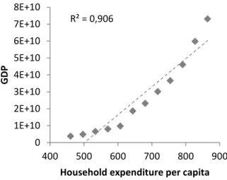
Fig. 3. Correlation between GDP and household expenditure per capita levels for Ghana year 1991/1992

and 2005/2006

Source: GDP data World Bank Indicators and GLSS1991/92 and 2005/2006

Fig. 4. Correlation between nightlight intensity and population on districts levels for Ghana year 2010

Source: DMSP-OLS processed by authors and population data provided by the World Bank

R² = 0,906 0 1E+10 2E+10 3E+10 4E+10 5E+10 6E+10 7E+10 8E+10 400 500 600 700 800 900 GD P

Household expenditure per capita

R² = 0,8628 0 10 20 30 40 50 60 0 50000 100000 di st ric t l ig ht /a rea District population/area 25

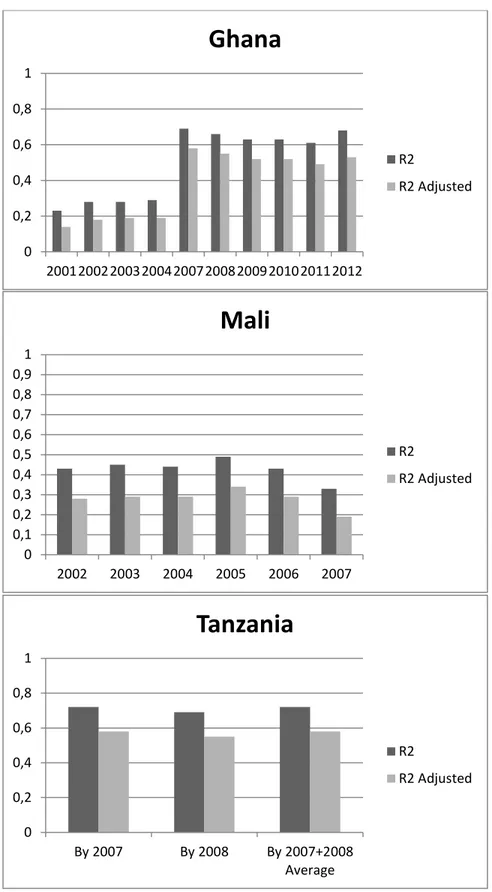
Fig. 5. GWR – Local R-squared for relationship between Dependent variable Total agricultural

production by district and Independent variable NDVI Intensity sum by district

Source: NDVI processed by authors and agricultural production data provided by the World Bank

0 0,2 0,4 0,6 0,8 1 2001200220032004200720082009201020112012

Ghana

Mali

Tanzania

Country Year R2 R2 Adjusted Ghana 2001 0,23 0,14 Ghana 2002 0,28 0,18 Ghana 2003 0,28 0,19 Ghana 2004 0,29 0,19 Ghana 2007 0,69 0,58 Ghana 2008 0,66 0,55 Ghana 2009 0,63 0,52 Ghana 2010 0,63 0,52 Ghana 2011 0,61 0,49 Ghana 2012 0,68 0,53 Mali 2002 0,43 0,28 Mali 2003 0,45 0,29 Mali 2004 0,44 0,29 Mali 2005 0,49 0,34 Mali 2006 0,43 0,29 Mali 2007 0,33 0,19 Tanzania 2007 0,72 0,58 Tanzania 2008 0,69 0,55

Table 1. GWR – Local R-squared for relationship between Dependent variable Total agricultural

production by district and Independent variable, sum of NDVI Intensity, by district

Source: NDVI processed by authors and agricultural production data provided by the World Bank