DESIGN OF A TECHNO-ECONOMIC
OPTIMIZATION TOOL FOR SOLAR
HOME SYSTEMS IN NAMIBIA
AKSEL HOLMBERG
OSCAR PETTERSSON
The School of Business, Society and Engineering
Course: Degree Project Course code: ERA400 Subject: Energy Technology Credits: 30
Program: M.sc Engineering in Sustainable
Energy Systems
Supervisor: Pietro Elia Campana, Mälardalen
University
Examiner: Bengt Stridh, Mälardalen University External partner: Abraham Hangula, Namibia
Energy Institute
Date: 2016-05-26 E-mail:
Ahg11008@student.mdh.se Opn11002@student.mdh.se
ABSTRACT
The expansion of the electrical grid and infrastructure is an essential part of development since it contributes to improved standard of living among the population. Solar home
systems (SHS) are one solution to generate electricity for households where the national grid does not reach or istoo sparsely populated to build a local mini-grid. Solar home system programs have been used as a solution for rural electrification in developing countries all over the world with various success, one of these countries is Namibia. A large fraction of the population in Namibia lacks access to electricity where most of the people live in rural areas not reached by the national electrical grid. However, several SHS clients in Namibia have been dissatisfied with their systems due to several issues regarding the service providers. Several service providers have limited technical know-how and therefore frequently over- and undersize system components and make mistakes during installations. An opportunity to improve SHS in Namibia is to develop a software tool that service provider can use to quickly calculate an optimum SHS in a user friendly way based on the electricity demands of the clients. An optimization model was developed using MS Excel which calculates the optimal SHS component capacities regarding cost and reliability with the use of Visual Basic macros. Various field studies and sensitivity analyses were conducted with the MS Excel model. The results were validated and compared with other software programs such as PVsyst and a Matlab model used in a previous study regarding solar power. Results show that several components in existing systems are incorrectly sized and that the MS Excel model could improve future installations and improve the reputation of SHS. The sensitivity analyses focused on cost, system reliability, system size and PV-module tilt and were implemented in the MS Excel model to optimize the results in a techno-economic perspective. The MS-Excel model was approved by Namibia Energy Institute and will be available for all service
providers in Namibia.
Key words: Solar home system, Optimization tool, PV, rural electrification, Optimization
ACKNOWLEDGEMENTS
The outcome of this thesis has been greatly benefitted from the help of several individuals who we would like to take this opportunity to thank.
We would first like to thank our supervisor Pietro Elia Campana for his guidance, technical know-how and support throughout the whole thesis. We would also like to thank Gustav Dahl scholarship at Mälardalen University for their financial support. We would also take this opportunity to thank Patrik Klintenberg for his knowledge of Namibia and helping us organizing the trip. Furthermore we would like to thank Abraham Hangula and Namibia Energy Institute for their help providing data and organizing all field studies in Namibia.
SUMMARY
This master thesis entitled “Design of techno-economic optimization tool for solar home systems in Namibia”, has focused on developing a MS Excel optimization tool for solar home systems in Namibia. This has been done by collaboration with Namibia Energy Institute and Mälardalen University. 8 weeks of research have been conducted in Windhoek, Namibia. During the time in Windhoek field studies and meetings with people with knowledge regarding the solar home systems have contributed to the development of the model to suit the situation in Namibia.
The current situation in Namibia is that a large fraction of households lack grid connection, both in cities and in rural communities. In the cities some households purchase expensive illegal electricity instead of investing in off-grid solutions and in the rural communities people use fossil energy sources.
The lack of technical know-how by the service providers when sizing and installing solar home systems have caused solar home systems to receive a bad reputation. This has made people doubtful about investing in solar home system.
The optimization model is developed in MS Excel which is a software that most service providers have available. The MS Excel optimization model has been developed to be as user friendly as possible and try to have few inputs as possible. The model has been developed from inspiration of previous research. To get an accurate optimization as possible Namibia is divided into three zones where the specific solar radiation for the largest city in each zone represents the solar radiation for the whole zone. The optimal tilt for each zone is calculated from a Matlab model used in a previous study. The result showed that the tilt should be 20o in the north, 25o in the central part of Namibia and 30o in the south. The model contains three load profiles that suit the client’s needs. The first load profile has a peak during the morning, lunch and one major peak in the evening. The second load profile has a major peak during the day and the third load profile has a major peak during the evening.
Fields studies have been conducted in order to test and validate the model. Three households have been inspected in Katutura, a suburb to Windhoek. The results from the inspections showed that service providers over- and undersize the systems. In one investigated case, the households had a greatly oversized inverter and in another case the household had
undersized cables. The oversized inverters caused the client to pay more for the system than necessary and the undersized cables caused high power transfer losses. During the
inspection, the clients that were satisfied with their system had similar systems to what the MS Excel optimization model calculated. The MS Excel model will be available for free for all SHS service providers in Namibia and can be downloaded from the website of Namibia Energy Institute.
CONTENT
1 INTRODUCTION ... 10
1.1 Overview ...10
1.2 Background ...10
1.2.1 Energy in Namibia ...11
1.2.2 Rural Electrification and Energy Use ...12
1.2.3 Solar Home Systems Overview ...13
1.3 Problem Definition ...15
1.4 Purpose ...16
1.5 Scope and Limitations ...16
1.6 Literature review ...16
1.6.1 Electric Load and Battery Capacity ...17
1.6.1.1 Loss of Load probability ... 18
1.6.2 Solar Module Efficiency ...19
1.6.3 Economy and sustainability ...20
1.7 Research questions ...22
2 METHODOLOGY ... 23
2.1 Research Design and Approach ...23
2.2 Literature Study ...23
2.3 SHS Data ...23
2.4 Software ...23
3 SOLAR HOME SYSTEM MODELING ... 24
3.1 Simulation ...24
3.1.1 Optimal tilt ...24
3.2 Optimization ...25
3.2.1 Load profile ...25
3.2.2 Approximate estimation of PV and battery ...26
3.2.3 Angle of incidence ...27
3.2.8 Main optimization macro ...32
3.2.9 Interface macros ...37
3.3 MS Excel model overview ...37
3.3.1 Inputs ...38
3.3.2 Results ...39
3.3.3 Errors and warnings ...40
3.4 Field study ...41
3.4.1 Modeling SHS for a bar ...41
1.1.1.1 Life cycle cost ... 43
3.4.2 Inspection of existing systems ...43
3.4.2.1 Simulation ... 44
3.4.3 Validation ...46
3.5 Sensitivity analysis ...47
3.5.1 Module tilt ...47
3.5.2 System reliability and size ...47
4 RESULTS ... 48
4.1 Model validation ...48
4.2 Field study of bar ...50
4.3 Field study of inspected systems ...52
4.4 Sensitivity analysis ...53
5 DISCUSSION... 61
5.1 Field study Usage ...61
5.2 Validation ...61 5.3 PV-module tilt ...61 5.4 Reliability ...62 5.5 Economy ...63 6 CONCLUSION ... 64 7 FUTURE RESEARCH ... 65 8 REFERENCES ... 66
COMPLETE LIST OF FIGURES AND TABLES
Figure 1 Energy sources in Namibian energy sector (Oertzen, 2015). ... 11
Figure 2 Global horizontal irradiation Namibia SolarGIS © 2016 GeoModel Solar. ...12
Figure 3 SHS schedule. ...14
Figure 4 Household with SHS in Katutura consisting of a 50 𝑊𝑝 solar module. ... 15
Figure 5 Loss of load probability (Azimoh, Wallin, Klintenberg, & Karlsson, 2014). ...19
Figure 6 Solar module tilts in South Africa (Azimoh, Wallin, Klintenberg, & Karlsson, 2014). ... 20
Figure 7 Cost flow for various energy sources for lighting (Oertzen, 2015). ...21
Figure 8 Economic gain in system used in an optimal way (Azimoh, Wallin, Klintenberg, & Karlsson, 2014). ... 22
Figure 9 Global horizontal irradiation divided into three zones, SolarGIS © 2016 GeoModel Solar. ... 25
Figure 10 Load profiles. ... 26
Figure 11 Daily average total global radiation against a horizontal surface (Meteonorm). ... 29
Figure 12 Flowchart of the optimization macro. ... 32
Figure 13 Optimization code. ... 33
Figure 14 Code for parallel and series combination for PV ... 34
Figure 15 Code for parallel and series combination for batteries. ... 36
Figure 16 Image of the main page of the MS Excel tool. ... 37
Figure 17 Load inputs. ... 38
Figure 18 Approximate estimation for PV and battery. ... 38
Figure 19 PV specifications. ... 39
Figure 20 Battery specifications... 39
Figure 21 Results for PV and battery. ... 40
Figure 22 Errors and warnings. ... 40
Figure 23 The inspected bar. ... 42
Figure 24 Cash flow diagram for the bar. ... 51
Figure 25 Monthly energy generation comparison between module tilts of 23o and 30o. ... 54
Figure 26 Load profile impact on optimal system size, household 1. ... 54
Figure 27 Load profile impact on optimal system size, household 2. ... 55
Figure 28 Module tilt impact on reliability and power generation, household 1. ... 55
Figure 29 Module tilt impact on reliability and power generation, household 2. ... 56
Figure 30 Module tilt impact on optimal module and battery size, household 1. ... 56
Figure 31 Module tilt impact on optimal module and battery size, household 2. ... 57
Figure 32 Reliability impact on optimal system size, household 1. ... 57
Figure 33 Reliability impact on optimal system size, household 2. ... 58
Figure 34 System size impact on system reliability, household 1. ... 58
Figure 35 Days of autonomy impact on optimal system size, household 1. ... 59
Table 1 Equipment and estimated load of the bar. ... 42
Table 2 Specifications and components chosen for optimization. ... 42
Table 3 Total investment cost for the bar ... 43
Table 4 Equipment and estimated load of household 1. ... 44
Table 5 Specifications for the currently installed SHS, household 1. ... 45
Table 6 Equipment and estimated load of household 2... 45
Table 7 Specifications for the currently installed SHS, household 2. ... 45
Table 8 Equipment and estimated load of household 3. ... 45
Table 9 Specifications for the currently installed SHS, household 3. ... 45
Table 10 Battery models simulated in PVsyst, household 1. ... 46
Table 11 PV modules simulated in PVsyst, household 1... 46
Table 12 Battery models simulated in PVsyst, household 2... 46
Table 13 PV modules simulated in PVsyst, household 2. ... 46
Table 14 PVsyst validation results, household 1... 48
Table 15 PVsyst validation results, household 2. ... 48
Table 16 Matlab validation results, household 1 and 2. ... 49
Table 17 Results, MS Excel optimization for the bar. ... 50
Table 18 Results of the life cycle cost analysis for the bar. ... 50
Table 19 Comparison of inspected system and results from MS Excel optimization, household 1. ... 52
Table 20 Comparison of inspected system and results from MS Excel optimization, household 2. ... 52
Table 21 Comparison of inspected system and results from MS Excel optimization, household 3. ... 53
NOMENCLATURE
Name Sign Unit
Annuity factor A %
Battery capacity Cbat Ah
Current I A
Efficiency η %
Energy E kWh or Wh
Interest rate i %
Inverter rating VA Volt*Ampere
Power P W Resistance R Ω Solar irradiance G W/m2 Time t hours Time n years Voltage U v
ABBREVATIONS
CC Charge Controller
DOD Depth of Discharge % (equals 1-SOC)
Eq Equation
LCOE Levelized Cost of Energy
LOLP Loss of Load Probability % (equals 1-reliability)
LPG Liquid Petroleum Gas
Mb Megabyte
NEI Namibia Energy Institute
NPV Net Present Value
N$/NAD Namibian Dollar (100 N$ = 53 SEK, 2016-05-16)
PBP Payback Period
PV Photovoltaic
PVWP Photovoltaic Water Pump
SHS Solar Home System
SOC State of Charge %
SRF Solar Revolving Fund
1 INTRODUCTION
This thesis is focusing on solar home systems in Namibia. In this chapter of the report, the background, problem definition, purpose, scope and a literature study will be presented.
1.1 Overview
One of the major challenges of our time is to provide poor rural areas with robust delivery of electricity. Sub-Saharan Africa is one of the poorest regions in the world and countries in the region are currently undergoing a strong economic growth. The expansion of the electrical grid and infrastructure is an essential part of development since it contributes to improved standard of living among the population. Renewable energy such as solar power has a large potential in sub-Saharan Africa and can play an important role to reach the United Nations development goals where one of the objectives is to ensure access to clean, reliable,
affordable and modern energy for all (African Clean Energy, 2016). A large number of the people live in rural areas far from a national electricity grid. Therefore, it is difficult to find economically viable solutions to electrify certain rural communities. Non-electrified households in sub-Saharan Africa uses fossil fuels such as kerosene, firewood and liquid petroleum gas as their main energy source. If these fuels can be replaced by renewable electricity it could contribute to a reduction of greenhouse gases along with increased sustainable development, health and comfort in Africa.
1.2 Background
Solar home systems (SHS) are one solution to generate electricity for households not reached by national grid or for areas too sparsely populated to build a local mini-grid. SHS programs have been used as a solution for rural electrification in developing countries all over the world with various successes, one of these countries is Namibia (Rämä, Pursiheimo, Lindroos, & Koponen, 2013).
Namibia has the second lowest population density in the world. A large fraction of the population in Namibia lacks access to electricity where most of the people live in rural areas where the national electrical grid does not reach.
In 2013 only 32% of Namibia’s total population of roughly 2 million had access to electricity (International Energy Agency, 2015). Even if a large fraction of the population is without electricity the annual electricity consumption has increased with an average of 5. 6%. From year 2000 to 2010 the electricity consumption has increased with 79%, but in the same time there have only been a small increase in the domestic electricity generation. The increased electricity consumption is supplied by imported electricity from neighboring countries
1.2.1 Energy in Namibia
Fossil energy sources such as diesel and petrol are the two main energy sources in the
Namibian energy sector as depicted in Figure 1. The second largest energy source is electricity which is both produced domestically and imported. Today the main source of the domestic generated electricity is hydro power.
Solar power currently has a minor contribution to the electricity production but is a growing source of energy in Namibia (Oertzen, 2015).
Figure 1 Energy sources in Namibian energy sector (Oertzen, 2015).
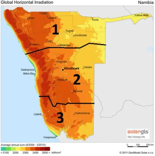
The Namibian Renewable Energy Program is an initiative from the government whose goal is to increase the access of affordable domestically generated renewable energy. This program is focusing on the rural areas without grid connection. The technology that will be mostly applied is off-grid solar energy technologies. Namibia is an arid country located relatively close to the equator and therefore has high solar irradiance levels in most areas during the year as illustrated in Figure 2. Due to the potential in solar power, various large and small scale photovoltaic (PV) projects have recently been constructed or planned. This will contribute to a reduction of Namibia’s dependence of imported energy. This will also contribute to the progress of national policy on climate change by increasing renewable energy generation (Center for clean air policy , 2012) (Oertzen, 2015).
Figure 2 Global horizontal irradiation Namibia SolarGIS © 2016 GeoModel Solar.
1.2.2 Rural Electrification and Energy Use
If there is no access to electricity, households rely on energy sources such as biomass, liquid petroleum gas, candles, paraffin and kerosene. These fuels are commonly used for lighting, cooking and space heating and accounts for 80% of the energy consumption in rural areas of sub-Saharan Africa (Gujba, Thorne, Mulugetta, Rai, & Sokona, 2012). The usage of fossil fuels indoors is a health risk, especially when used for cooking and causes approximately 4 million annual deaths worldwide (African Clean Energy, 2016). Household use of fossil fuels is also a major environmental problem since it also contributes to greenhouse gas emissions and deforestation (Oertzen, 2015). Another issue is informal settlements in the outskirts of urban areas. The government refuses to connect these areas to the grid in order to prevent further urbanization. Cables might be dragged from grid connected electrified households close by where the owner makes a business by selling power illegally (Hanghome, 2016). As previously stated energy poverty is a major challenge in Namibia where only 32 % of the population had access to electricity in 2013. However most of the population with electricity
Electrification improves the health and comfort for the household. It also contributes to development since the household can have brighter light during the night to do activities such as studies or run local businesses. The household could also charge their phones or connect appliances such as radio and TV (Jain, Jain, & Dafhana, 2014).
There are two possible ways to electrify these areas, either grid connection or off-grid solutions. When the grid is extended to new villages a large number of the households lack the economical availability to connect to the grid. In some cases only 40% of the households in a village connect to that extended grid. The households in the rural areas have low
electricity consumption comparing to the urban households but demand the same services. This makes it unprofitable to extend the grid to the rural areas (Jain, Jain, & Dafhana, 2014). The alternative to grid connection is off-grid solutions with energy sources such as solar, wind, biogas etc. If the rural village is dense enough, a mini-grid is usually constructed where the village is electrified with small solar parks and diesel generators as an example. If a mini grid is not a preferred solution, a SHS is an option where the household generates their own electricity (Jain, Jain, & Dafhana, 2014).
1.2.3 Solar Home Systems Overview
A program for increasing the usage of SHS was developed in Namibia 2003 by the ministry of mines and energy with support from the United Nations development program and the global environment facility. Ministry of mines and energy administrates the Solar Revolving Fund (SRF) which purpose is to increase and improve rural electrification with solar power by offering minor loans and to overlook all SHS service providers. The loan is limited at N$ 35 000 (19 000 SEK, 2016-05-16) for a SHS with an interest rate at 5% (Jain, Jain, & Dafhana, 2014). Larger loans can be taken from various banks such as Bank Windhoek (Amakutsi, 2015). Ministry of mines and energy has also developed the Namibian code of practice which is a guideline on how installations and system sizing of SHS and other solar technologies is made properly.
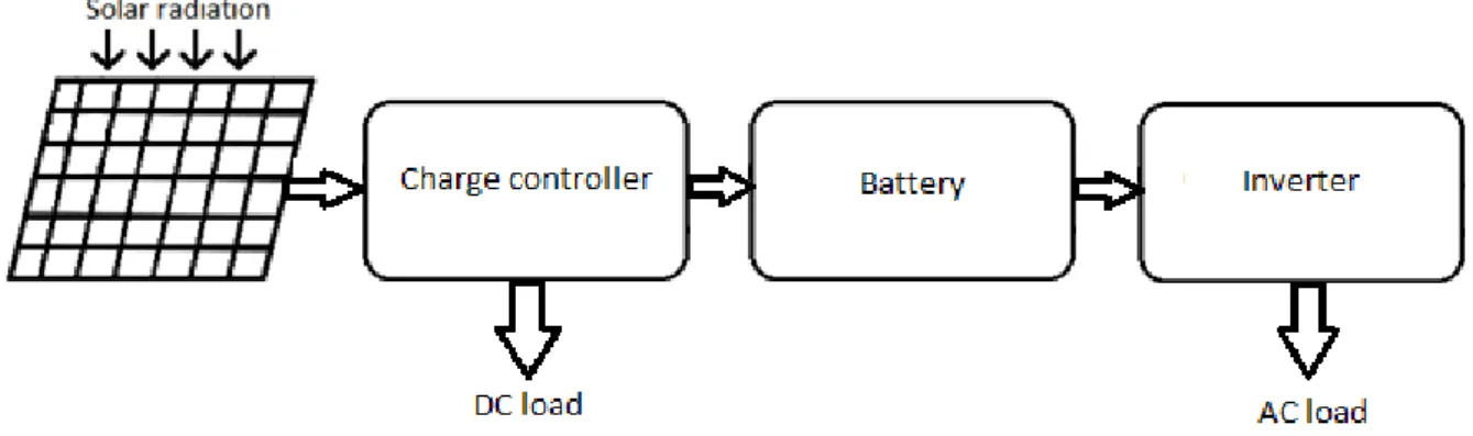
A SHS usually consist of three major sections, PV module, battery set and electricity load. A basic scheme can be seen in Figure 3.
Figure 3 SHS schedule.
The electricity generation consists of a PV module with solar cells connected in series or parallel dimensioned to match the battery capacity and the household load. The module is mounted on a support structure on the roof of the house or a pole on the ground with a preferred orientation and tilt (Diessen, 2008).
The energy and storage system consists of three major components, a charge control unit, a battery and an inverter if the household is using alternating current (AC) equipment. The charge controller is used to protect the battery from inappropriate use and increase the life span since it transforms the voltage and current from the module to a level that is safe for the battery to handle. The charge controller will cause temporary power outages if the system is used incorrectly. The battery in the solar home system stores some of the electricity produced by the PV-module in order to provide the household with electricity at any point during the day. The batteries are usually lead-acid deep charge batteries. The inverter is used to convert direct current (DC) generated by the modules to AC with a voltage which is used by most electrical equipment. (Diessen, 2008). A system that only uses DC equipment is also common and does not require an inverter (Energypedia, 2015). An informal household using SHS with a 50 𝑊𝑝 solar module in the suburb Katutura in Windhoek is depicted in Figure 4.
Figure 4 Household with SHS in Katutura consisting of a 50 𝑊𝑝 solar module.
1.3 Problem Definition
SHS is a solution that could reduce the use of fossil energy sources and illegally sold power in Namibia. A vast majority of the SHS installations are not done properly (Amakutsi, 2015). Problems include having wrong module tilt, cable size, battery size and PV size and making various mistakes during the installations. The load of the user has to match the size of the PV modules and battery size. This have to be done in an optimal techno-economical perspective based on the income and load demand of the household. Another issue is the quotations that the service providers make for a specific client. Quotations are suggestions of a complete system for a client where load estimation, components and all costs are listed. SRF receive the quotations from the service providers and have to deny or approve them. The quotations are often too inaccurate to determine a relatively accurate load demand. A load estimation and system sizing for a SHS might solely be based on the knowledge that the client wants to power a couple of light bulbs and a TV. The client usually has limited knowledge regarding solar power and it is the responsibility of the service providers to provide them with sufficient information and install the systems correctly (Amakutsi, 2015). However, some service providers are not interested to invest time and work into their client. An example of this is that some installers use the naked eye to determine the orientation and tilt of the PV module rather than using simple tools (Hanghome, 2016). Service providers with limited technical know-how that makes sloppy installed and incorrectly sized systems have contributed to several reports of unsatisfied clients. Additionally, insurance companies are refusing to insure the systems (Amakutsi, 2015). The installations have been improved since the SRF started to investigate SHS installations. However, many problems still remain and more can be done to improve the SHS in Namibia. The service providers does not have access to
advanced or commercial software tools such as Matlab or PVsyst when making installations, instead some use rough estimations without having the Namibian code of practice in
consideration (Hanghome, 2016). This is one of the reasons that one or more SHS
components might be incorrectly sized. Undersized PV modules or batteries will cause power shortages, undersized inverters or charge controllers will overheat and break and undersized cables will cause high power transfer losses. Oversized components will contribute to
unnecessary expenses for the usually poor households (Hanghome, 2016).
1.4 Purpose
The purpose of this thesis is to inspect SHS and evaluate available data to find opportunities to achieve more efficient and sustainable rural electrification. This will be achieved by creating a SHS model with a common software tool such as MS Excel that SHS service providers can use to optimize all SHS installations in a quick and user friendly way. The goal is to reduce the amount of incorrectly sized and sloppy installed SHS and contribute to the development of the technology and help people in Namibia to increased living standards by applying knowledge in energy systems.
1.5 Scope and Limitations
The work will focus on optimizing the systems with empirical data by developing an
optimization tool and using simulation programs. The scope will be on SHS using AC loads, which means an inverter is always included in the system. No hybrid systems or other solar power technologies such as solar water heaters will be considered.
There will be no study in how SHS will affect the living standard for the people who are going to install or has installed SHS. Additionally, there will be no research into various payment methods.
1.6 Literature review
Previous studies show that there is a great potential for households to invest in a SHS. However, roughly 56% of rural households in neighboring South Africa using SHS were not satisfied (Azimoh, Klintenberg, Wallin, & Karlsson, 2015) and several reports of dissatisfied customers have been reported in Namibia as well (Amakutsi, 2015).The bad reputation causes rural household to refrain from investing in SHS and rather keep using fossil fuels and wait until a stable national grid becomes available (Azimoh, Klintenberg, Wallin, & Karlsson, 2015).
1.6.1 Electric Load and Battery Capacity
A common problem is that SHS does not meet the demand of the household. According to study conducted in South Africa, 50-90 % of the households, depending on which village they reside in reported that their energy needs were not fulfilled (Azimoh, Klintenberg, Wallin, & Karlsson, 2015).
Another study conducted in Tanzania is listing several issues regarding the household load. A few examples are the use of inefficient power consuming equipment and service providers ignoring load demand estimation before the installation (Kulworawanichpong &
Mwambeleko, 2015). If a system is designed for powering two light bulbs and the system is working fine the user might connect additional equipment. They might also use inefficient power consuming equipment or use it for a longer period of time during the day
(Kulworawanichpong & Mwambeleko, 2015). If the load limits are violated, the charge controller will cause a power outage resulting in that the users cannot use their equipment. This will sometimes cause the users to bypass the charge controller and connect the load directly to the battery which will reduce the life span. Frequent power outages cause dissatisfaction among users and a bad public opinion (Azimoh, Klintenberg, Wallin, & Karlsson, 2015).
Larger SHS that can meet a higher load demand is more costly and a majority of the users are poor and cannot afford larger systems. However, even if a larger system was installed this issue could still remain, no matter the size, as long as the clients overload the system. A study made in Cambodia 2008 suggested to make a sealed box for the components that protects the equipment from being tampered. The box has a display that shows the current state of charge of the battery (Diessen, 2008).
Battery replacements are costly and frequent battery replacements are one of the major contributors to a high operation and maintenance cost for a SHS. An expensive battery replacement motivates the household to buy cheaper batteries or a car battery rather than a preferred deep cycle battery. It has also been reported that SHS owners replace their
equipment with cheap and illegal components or connect another battery with different characteristics in series with the previous one (Azimoh, Klintenberg, Wallin, & Karlsson, 2015) (Tanzanian affairs, 2007).
When the battery is being discharged and recharged it is known as a cycle and corresponds roughly to one day for deep cycle batteries. The life of the battery increases, the lower each discharge is. Usually the charge controller is set to a charge limit of 50% to keep a decent life span (Woodbank Communications Ltd, 2016). If the charge limit would be set higher the life span of the battery would increase but a battery with more capacity would be required. If the discharge limit is surpassed, the charge controller will cause a power outage until the battery is recharged to a safe level. The reason that batteries wears out by being too discharged is due to chemical reactions which causes lead sulfate diode in the battery to crystallize. The diode crystallizations are not reversible and will aggravate the charging of the battery (Woodbank Communications Ltd, 2016). The battery also gets worn out when the users are connecting to much electric load on the battery during a specific time. Unlike car batteries, deep cycle batteries are built to have low and constant charges and discharges. The charge controller
will then also cause a power outage a few minutes at a time until the load is at a safe level. These are the reasons why the charge controller is being bypassed by inexperienced users or maintenance workers. The household can then discharge the battery below 50% until the voltage becomes too low. The household can also use too high loads at the same time (Kulworawanichpong & Mwambeleko, 2015). Solutions for the battery issue have been to maximize the efficiency without consideration of the cost and vice versa. For example a study in Senegal 2015 proposed to recycle old cellphone batteries and make them into a solar battery by connecting them in series (Diouf, 2015). Another solution has been to instead maximize the efficiency with expensive solar storage systems from Tesla (Oertzen, 2015). Other component issues include poor wiring with loose connections, unnecessary long or undersized cables. Another problem is poor system maintenance and cleaning which results in dusty solar modules or dirty and clogged battery terminals. The temperature also affects the battery with higher temperatures decreasing the battery life span (Electopaedia, 2005).
1.6.1.1 Loss of Load probability
Loss of load probability (LOLP) is the amount of time during a specific period that the household is experiencing power outages. With an optimized SHS where the household does not violate the load limit, LOLP can be close to zero. According to a study in South Africa, if the system is overloaded the loss of load probability could become approximately 70% when the PV is placed on the ground and tilted 0o and the household is using more power than the system is designed for. For the standard system usage, the PV is also tilted at 0o and this will give a LOLP at 46.6%. The optimal system resulted in a LOLP at 0% where the module is tilted at 14oor 34o depending on the season in order to maximize the annual power output and the household is having a lower load. Figure 5 shows LOLP based on the household usage in consideration of load and module tilt of the three cases (Azimoh, Klintenberg, Wallin, & Karlsson, 2015).
Figure 5 Loss of load probability (Azimoh, Wallin, Klintenberg, & Karlsson, 2014).
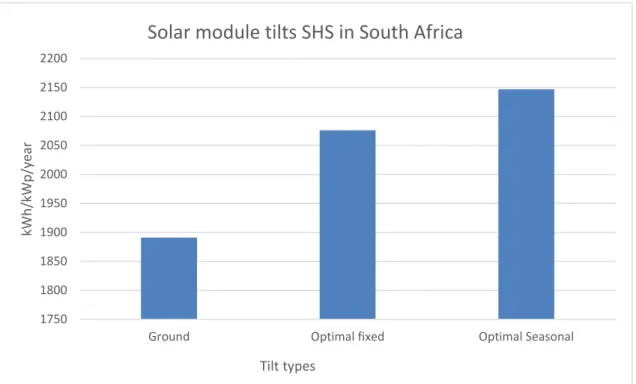
1.6.2 Solar Module Efficiency
A previous study in South Africa examines what impact the tilts of the modules have on the system performance. A comparison was made if the solar module were placed directly on the ground (0o tilt), optimized at the most efficient annual tilt or an optimized tilt that varies for each season as depicted in Figure 6 (Azimoh, Wallin, Klintenberg, & Karlsson, 2014). The seasonal tilt was changed with the use of a manual clamp arm attached to the solar module in order to match the seasonal solar altitude. The study also shows that the annual optimal tilt was roughly the same as the latitude, in this case around 24o. Including a solar tracking device on the PV-module improved the efficiency and power generation of the system but was too expensive and complex to be a sustainable solution for SHS. The improved tilt only displayed a small decrease in loss of load probability of 1.3 % for an overloaded system. The reduced LOLP as a result of improvements regarding module tilt increased if the system is used in a more optimal way (Azimoh, Wallin, Klintenberg, & Karlsson, 2014).
0% 10% 20% 30% 40% 50% 60% 70% 80%
Overloaded Standard Optimized (0% LOLP)
Pro b ab ili ty System usage
LOLP
Figure 6 Solar module tilts in South Africa (Azimoh, Wallin, Klintenberg, & Karlsson, 2014). The solar module does not only have to be mounted in the right tilt and orientation. The mounting have to withstand harsh weather conditions and risk of theft. Another common mistake is that the module is mounted directly on the roof which prevents natural passive cooling. This causes the operating temperature to be roughly 10o C higher on average and thereby reducing the efficiency (PVeducation, 2015). The optimal solution is to have space between the PV module and the roof and to use aluminum fins to transfer heat from the module. Shading is also an issue when mounting the solar module. Shading can be avoided by mounting the module with a pole instead of on the roof (PVeducation, 2015).
1.6.3 Economy and sustainability
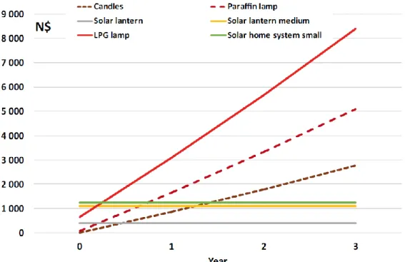
Electrification with SHS could not only increase the health and comfort for the users, it could also be an economic gain. Figure 7 shows cost flow for various energy sources for lighting where the y axis is the total cost and x axis is the amount of years. The figure shows that SHS is cheaper than commonly used fossil energy sources if the system is working for three years without any maintenance costs.
1750 1800 1850 1900 1950 2000 2050 2100 2150 2200
Ground Optimal fixed Optimal Seasonal
kW h /kW p /y ear Tilt types
Figure 7 Cost flow for various energy sources for lighting (Oertzen, 2015).
Companies providing SHS in South Africa have withdrawn due to limited profits as a result of delayed or ceased payments from dissatisfied customers (Azimoh, Klintenberg, Wallin, & Karlsson, 2015).
In the study the study performed by Aziomoh,Klintenberg, Wallin & Karlsson (2015) The economic impact of households in three villages using SHS was evaluated. The study was made with a preferred energy burden at 10% which is the share of the household’s income that is used for energy. The SHS costs were compared to candle, paraffin and liquid
petroleum gas. The results of the study showed that it was difficult to notice if the SHS had any positive impact of the household economy. Few new job opportunities were created as a result of SHS and only 23% of the SHS clients reported it having a positive impact on their household economy (Azimoh, Klintenberg, Wallin, & Karlsson, 2015).
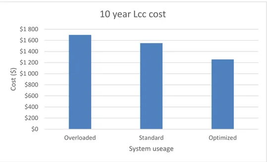
The study displayed various potential economic gains if the systems were used in an optimal way. The 10 year life cycle cost of an optimized system could be as low as 1257 $ compared to 1700 $ with an overloaded system as shown in Figure 8. This corresponds to a 33% reduced life cycle cost and 26 % reduced annualized costs (Azimoh, Wallin, Klintenberg, & Karlsson, 2014).
Figure 8 Economic gain in system used in an optimal way (Azimoh, Wallin, Klintenberg, & Karlsson, 2014).
In a study conducted in China, a tool for optimizing photovoltaic water pumping (PVWP) systems used for crop irrigation was developed. The model uses a generic algorithm in Matlab in order to calculate the optimum PVWP system size to maximize the crop yield and annual profit while maintaining a system reliability of 100%. The results showed that the PV-modules used in previous systems were oversized. If the PV-PV-modules were sized correctly according to the results of the Matlab model, the investment capital cost could decrease with 18. 8% and improve the economic feasibility of PVWP systems (Campana, o.a., 2015).
1.7 Research questions
Previous studies show that there are multiple problems with SHS but also opportunities for improvements. Questions that will be answered in this thesis are listed below.
How can a SHS be optimized?
What are the optimal sizes of SHS for the households from techno-economic point of view? $0 $200 $400 $600 $800 $1 000 $1 200 $1 400 $1 600 $1 800
Overloaded Standard Optimized
Cos
t
($)
System useage
2 METHODOLOGY
In this chapter the methodology for this thesis work is explained. The research design and approach is explained first, followed by the data collection method and the software being used.
2.1 Research Design and Approach
The method that is used for this thesis work has an inductive approach. Which means that the study is based on the problems that are identified and then facts and theory are applied in order to develop a better understanding for the problems and the results. The inductive approach can be more time consuming than other methods due to the analysis that is required. The analysis could lead to findings of new theories which mean that additional information and literature needs to be reviewed in order to understand the results and possible future unknown problems during the work (Blomkvist & Hallin, 2014). As an example, the purpose to develop a software tool to improve SHS was not the solution until further investigation and meetings in Namibia.
2.2 Literature Study
The literature study for this thesis is important in order to understand the context of the problem and to get a better picture of the field of study. The information was gathered from previous research studies conducted at locations where the conditions are similar to the society and environment in Namibia.
The scientific papers used for the literature study were collected from electronic sources and online databases such as Google scholar, Diva, Science direct and Scopus. Other documents and oral sources were collected from NEI and SRF.
2.3 SHS Data
Data for the existing systems is available at NEI and SRF with quotations, reports, invoices and previous studies regarding SHS in Namibia. Data for the field studies were gathered from inspections of clients currently using or planning to install SHS. A data logger for measuring power consumption and an angle meter was used to determine PV tilt was used.
2.4 Software
The model was developed in MS Excel by using macro functions. The coding was developed using the sequential coding program Visual Basics which is included in MS Excel. PVsyst and
Matlab are used to validate the model. PVsyst is a commercial software used to simulate and size small and large scale PV-systems. The radiation and temperature data was gathered using Meteonorm.
3 SOLAR HOME SYSTEM MODELING
In this chapter a description of the equations used and how they were implemented into MS Excel in order to develop a SHS optimization model is presented. The optimization model is then compared to PVsyst and a Matlab model with results from field studies in order to validate the results from the developed optimization tool. Additionally a sensitivity analysis is conducted.
3.1 Simulation
Some of the equations used in the MS Excel model are partly from a previous study
conducted in China (Campana, o.a., 2015). A Matlab model used in the study was adjusted to find the optimal tilt for the PV for various locations in Namibia. It is also used for validation and investigating existing systems in the field study to find the reliability, PV power
generation, efficiency and other parameters for a specific SHS (Campana, o.a., 2015).
3.1.1 Optimal tilt
Namibia is divided into three zones in the code of practice where each zone has a
recommended tilt that service providers should take in consideration when installing systems (NAMREP, 2006). From zone 1 to 3, the recommended tilt was 25 o, 30 o and 35o. Simulations were made in Matlab to find the optimal tilt for the latitude of a major city in each region (Tsumeb, Windhoek and Ketmanshoop) that can be seen in Figure 9. The code tried all tilts when the module was facing north between a certain intervals and stored the optimum value. The optimal tilt is the one resulting in the highest annual power output and the most evenly distributed power output over the whole year.
Figure 9 Global horizontal irradiation divided into three zones, SolarGIS © 2016 GeoModel Solar.
3.2 Optimization
The goal of the optimization model is to find the optimal SHS size regarding cost and reliability for a specific load. The optimization code were written in Visual Basic and then applied as multiple macros in the MS Excel worksheet.
3.2.1 Load profile
The load is based on the equipment being used in the household, how many hours per day and the power consumption of the equipment. The data is acquired from quotations that the service providers have made for a client. The load has to be approximately estimated since the quotations do not always contain sufficient information. An approximated standard load profile was created based on a previous study conducted in Algeria with load peaks during morning, lunch and a major peak during the evening (Kaabeche, Belhamel, & Ibtiouen, 2011). There is a minor constant load during the rest of the day, the same daily load profile were used every day of the year. Two additional load profiles were created, one with higher loads during daytime representing day time businesses and a load profile with higher load during
evening and night which represents night time businesses such as bars. The load profiles are illustrated in Figure 10.
Figure 10 Load profiles.
3.2.2 Approximate estimation of PV and battery
An approximate estimation of required nominal PV power (
𝑃
𝑃𝑉) and battery was calculated directly from the load estimation. This was in order to estimate the system size. Theapproximate estimation was also used for the optimization. The optimization will test PV and battery sizes around the estimation to find the optimal PV and battery sizes. This will
decrease the execution time for the model. Estimations of nominal PV power (
𝑃
𝑃𝑉)) werecalculated from Eq 1 (Sendegeya, 2016).
𝑷𝒑𝒗(𝒌𝑾𝒑) =
𝑬𝒍𝒐𝒂𝒅
𝜼𝒓𝒕∗ 𝜼𝑺𝑻𝑪∗ 𝜼𝑪𝑪∗ 𝜼𝒊𝒏𝒗𝒆𝒓𝒕𝒆𝒓 𝑻𝒔𝒐𝒍𝒂𝒓
Eq 1
Where
𝐸
𝑙𝑜𝑎𝑑 is the daily load in kWh/day, 𝜂𝑟𝑡 is the battery round trip efficiency (75%), 𝜂𝑆𝑇𝐶 is the de-rating factor (90%), 𝜂𝐶𝐶 is the charge control efficiency (95%) and 𝜂𝑖𝑛𝑣𝑒𝑟𝑡𝑒𝑟 is the inverter efficiency (90%). The efficiencies are assumed to represent all power losses from the peak power output of PV module to the electric appliances. This is divided by the average peak solar output time (𝑇
𝑠𝑜𝑙𝑎𝑟)
during the worst month of the year (February) which is assumed to be 6 hours/day. Battery capacity is calculated from Eq 2 (Sendegeya, 2016).0 10 20 30 40 50 60 70 80 90 100 1 2 3 4 5 6 7 8 9 10 11 12 13 14 15 16 17 18 19 20 21 22 23 24 Po w er u sage (W) Hour
Daily load profiles for 1 kWh daily power consumption
Where
𝐸
𝑙𝑜𝑎𝑑 is the daily load in kWh,𝑈
𝑏 is the battery bus voltage, d is days of autonomy and𝐶𝐶
𝑙𝑖𝑚𝑖𝑡 is the state of charge limit of the charge controller limit which is at 50 % according tothe code of practice (NAMREP, 2006). The results from these approximations are only used to get a rough idea of the system size and to reduce the simulation time and should not be considered as final result since it might deviate greatly from the optimal result.
3.2.3 Angle of incidence
The angle of incidence towards a surface describes the angle solar rays make with the normal of the solar module. The angle of incidence (𝜃) for direct solar radiation on any surface at a given place and a given time were calculated using Eq 3.
𝜃 = 𝑎𝑟𝑐𝑜𝑠(𝑐𝑜𝑠(𝛿) ∗ 𝑠𝑖𝑛(𝜔) ∗ 𝑠𝑖𝑛(𝛽) ∗ 𝑠𝑖𝑛(𝛾) + 𝑐𝑜𝑠(𝛿) ∗ 𝑐𝑜𝑠(𝜔) ∗ 𝑠𝑖𝑛(𝜆) ∗ 𝑠𝑖𝑛(𝛽) ∗ 𝑐𝑜𝑠(𝛾) − 𝑠𝑖𝑛(𝛿) ∗ 𝑐𝑜𝑠(𝜆) ∗ 𝑠𝑖𝑛(𝛽) ∗ 𝑐𝑜𝑠(𝛾) + 𝑐𝑜𝑠(𝛿) ∗ 𝑐𝑜𝑠(𝜔) ∗ 𝑐𝑜𝑠(𝜆) ∗ 𝑐𝑜𝑠(𝛽) + 𝑠𝑖𝑛(𝛿) ∗ 𝑠𝑖𝑛(𝜆) ∗ 𝑐𝑜𝑠(𝛽))
Eq 3
Where β is tilt of the module and 𝜆 is the latitude. δ is the angle declination of the equator at a given day of the year (n) and calculated with Eq 4.
𝛅 = 𝟐𝟑. 𝟒𝟓 ∗ 𝒔𝒊𝒏 (𝟑𝟔𝟎 ∗ (𝟐𝟖𝟒 + 𝒏)
𝟑𝟔𝟓 )
Eq 4
Where 𝜔 is the hour angle and describes the displacement of the sun due to the rotation of earth. The rotational speeds corresponds to approximately 15o per hour and calculated every hour (hh) and minute (mm) during the day using Eq 5.
𝝎 = ((𝒉𝒉 − 𝟏𝟐) + 𝒎𝒎 / 𝟔𝟎) ∗ 𝟏𝟓 Eq 5
However, the time is defined from the time zone in Namibia and needs to be adjusted to solar time using Eq 6.
𝑺𝒐𝒍𝒂𝒓 𝒕𝒊𝒎𝒆 – 𝒏𝒐𝒓𝒎𝒂𝒍 𝒕𝒊𝒎𝒆 = 𝟒 ∗ (𝑳𝒔𝒕− 𝑳𝒍) + 𝑬𝑸𝑻 Eq 6 Where Lst is the time zone standard meridian positive to the west and Ll is the local meridian. EQT is the equation of time and calculated with Eq 7.
𝑬𝑸𝑻 = 𝟐𝟐𝟗. 𝟐 ∗ (𝟎. 𝟎𝟎𝟎𝟎𝟕𝟓 + 𝟎. 𝟎𝟎𝟏𝟖𝟔𝟖 ∗ 𝒄𝒐𝒔(𝑩) − 𝟎. 𝟎𝟑𝟐𝟎𝟕𝟕 ∗ 𝒔𝒊𝒏(𝑩)
− 𝟎. 𝟎𝟏𝟒𝟔𝟏𝟓 ∗ 𝒄𝒐𝒔(𝟐 ∗ 𝑩) − 𝟎. 𝟎𝟒𝟎𝟖𝟗 ∗ 𝒔𝒊𝒏(𝟐 ∗ 𝑩)) Eq 7 Where angle B is calculated using Eq 8.
𝑩 = 𝟑𝟔𝟎 ∗ (𝒏 − 𝟏) 𝟑𝟔𝟓
Eq 8 Combining the two equations gives the hour angle adjusted to solar time (Eq 9).
𝝎 = 𝟏𝟓 ∗ (𝒉𝒉 − 𝟏𝟐) + 𝒎𝒎 + 𝑬
𝟒 + (𝑳𝒔𝒕 − 𝑳𝒍) Eq 9
Where 𝛾 is the solar azimuth angle, which is the angle between the sun and south, it is calculated from Eq 10. = 𝒂𝒓𝒄𝒄𝒐𝒔 (𝐜𝐨𝐬(𝜹) ∗ 𝐜𝐨𝐬(𝝎) ∗ 𝐬𝐢𝐧(𝝀) − 𝐬𝐢𝐧(𝜹) ∗ 𝐜𝐨𝐬(𝝀) 𝐜𝐨𝐬(𝜶) ) ∗ 𝝎 |𝝎| Eq 10
Where α is the solar altitude which is calculated using Eq 11.
𝛂 = 𝒂𝒓𝒄𝒔𝒊𝒏(𝒄𝒐𝒔(𝜹) ∗ 𝒄𝒐𝒔(𝝎) ∗ 𝒄𝒐𝒔(𝝀) + 𝒔𝒊𝒏(𝜹) ∗ 𝒔𝒊𝒏(𝝀)) Eq 11
3.2.4 Total radiation towards module surface
Direct beam solar radiation perpendicular to the sun is measured with a pyrheliometer and the total global radiation towards the ground is measured with a pyranometer.
The difference between these two variables equals the total diffuse radiation. This is the data required to perform radiation calculations at any angle and surface (Mälardalens högskola, 2010).
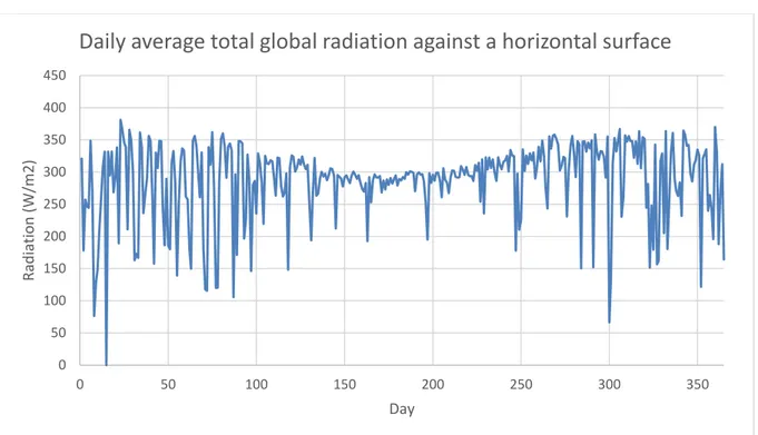
The irradiance data for various locations in Namibia were gathered using Meteonorm. The total radiation against the PV surface (G) is calculated using Eq 12.
𝑮 (𝑾/𝒎𝟐) = 𝑮
𝒃 + 𝑮𝒅 + 𝑮𝒈 Eq 12
Where 𝐺𝑏 is the global total beam radiation and is calculated using Eq 13. 𝑮𝒃(𝑾/𝒎𝟐) = 𝑮
𝒃,𝒏∗ 𝒄𝒐𝒔(𝜽) Eq 13
Where 𝜃 is the angle of incidence and 𝐺𝑏,𝑛 is global beam normal radiation calculated with Eq
14.
𝑮𝒃,𝒏(𝑾/𝒎𝟐) = 𝑮𝒃,𝒉
𝒄𝒐𝒔(𝜽𝒛)
Eq 14 Where 𝜃𝑧 is the angle of incidence from the zenith and 𝐺𝑏,ℎ is the global beam horizontal radiation, calculated using Eq 15.
𝑮𝒃,𝒉(𝑾/𝒎𝟐) = 𝑮
𝒉 − 𝑮𝒅,𝒉 Eq 15
Global total diffuse radiation 𝐺𝑑 is calculated using Eq 16.
𝑮𝒈 (𝑾/𝒎𝟐) = 𝝆𝒈∗ 𝑮𝒉∗ (𝟏– 𝒄𝒐𝒔(𝜷))
𝟐
Eq 17 Where ground reflectance constant (𝜌𝑔) is assumed to be 20%. The annual average daily global total solar irradiation against a surface (G) in Windhoek can be seen in Figure 11.
Figure 11 Daily average total global radiation against a horizontal surface (Meteonorm).
3.2.5 PV efficiency and power generation
The efficiency and electricity generation of a PV-module will be explained in this section. The efficiency of a PV-module varies with the temperature. Eq 18 is used to calculate the
operating efficiency for the PV module at a specific hour. 𝜼𝒑𝒗(%) = 𝜼𝒑𝒗,𝑺𝑻𝑪∗ (𝟏 + 𝝁 𝜼𝒑𝒗,𝑺𝑻𝑪∗ (𝑻𝒂− 𝑻𝑺𝑻𝑪) + 𝝁 𝜼𝒑𝒗,𝑺𝑻𝑪∗ 𝑵𝑶𝑪𝑻 − 𝟐𝟎 𝟖𝟎𝟎 ∗ (𝟏 − 𝜼𝒑𝒗,𝑺𝑻𝑪)) ∗ 𝑮 Eq 18
where, 𝜂𝑝𝑣,𝑆𝑇𝐶 is the efficiency of the PV module at standard test conditions (STC), 𝑇𝑎 is the ambient temperature and TSTC is the STC temperature (25o C) and
NOCT is the nominal operating cell temperature which is usually around 45o C. µ is the temperature coefficient of the power output which is calculated with Eq 19.
µ (%/°𝐂) ≈ 𝜼𝑺𝑻𝑪
µ𝑽𝒐𝒄
𝑽𝒎𝒑 Eq 19
where, µ𝑉𝑜𝑐 is the open circuit voltage temperature coefficient (V/°C) and
𝑉𝑚𝑝 is the maximum voltage point. To calculate the amount of electricity the PV-module can
generate, Eq 20 is used: 0 50 100 150 200 250 300 350 400 450 0 50 100 150 200 250 300 350 Rad iat ion (W/m2) Day
𝑷𝑷𝑽 (𝑾) = 𝒏𝑷𝑽∗ 𝑨𝑷𝑽∗ 𝑮 Eq 20 The area (𝐴𝑃𝑉) for the PV module is calculated from the STC using Eq 21. STC are at an irradiance of GSTC=1000 W/m2, cell temperature at 25° and angle of incidence at 0°. The nominal PV power output at STC (𝑃𝑝𝑒𝑎𝑘)is measured in kilowatt peak (kWp) and is a common unit to describe the size of a PV module.
𝑨𝑷𝑽 (𝒎𝟐) =
𝑷𝒑𝒆𝒂𝒌 𝜼𝑷𝑽∗ 𝑮𝑺𝑻𝑪
Eq 21
3.2.6 Battery
The state of charge (SOC) during a time t of the battery is calculated every hour for a whole year. Eq 22 and Eq 23 is the battery charge and discharge equation respectively (Campana, o.a., 2015). 𝑺𝑶𝑪(𝒕) = 𝑺𝑶𝑪(𝒕 − 𝟏) ∗ (𝟏 − 𝝈) + (
𝑬
𝒍𝒐𝒂𝒅(𝒕) 𝜼𝒊𝒏𝒗 − 𝑬𝑮𝒆𝒏(𝒕)) ∗ 𝜼𝑩 Eq 22 𝑺𝑶𝑪(𝒕) = 𝑺𝑶𝑪(𝒕 − 𝟏) ∗ (𝟏 − 𝝈) − (−𝑬
𝒍𝒐𝒂𝒅(𝒕) 𝜼𝒊𝒏𝒗 + 𝑬𝑮𝒆𝒏(𝒕)) Eq 23 Where, t is time in hours; 𝜎 is the self-discharge rate (0. 02 % per hour); 𝜂𝑖𝑛𝑣 is the efficiency of the inverter (if any) and 𝜂𝐵 is the charging efficiency of the battery. The constraints for the charge and discharge process can be seen below:𝑆𝑂𝐶 ≥ 100% = Only discharge
𝑆𝑂𝐶 < 100% & 𝑆𝑂𝐶 > 𝐶𝐶 𝑙𝑖𝑚𝑖𝑡 = Charge or discharge 𝑆𝑂𝐶 ≤ 𝐶𝐶 𝑙𝑖𝑚𝑖𝑡 = Only charge
If the power generated from the PV module, 𝐸𝐺𝑒𝑛(𝑡) is larger than the load, 𝐸𝐿(𝑡) and the
battery is not fully charged, the battery will be charged. If the load is larger than the
generated power and the state of charge is above the charge control limit, the battery will be discharged. If the SOC is below the charge control limit (CC limit), there will be a power outage during that hour and every hour during the year with a power outage is stored and used to calculate the total reliability.
The life span of the battery can be approximately calculated using Eq 24 (Azimoh, Wallin, Klintenberg, & Karlsson, 2014).
Where T is the operating temperature and DOD is the average highest depth of discharge during each cycle.
3.2.7 Cables
Sufficient cable sizes are required to reduce power transmission losses. Three wiring sections will be calculated including the cables connecting the solar modules to the charge controller, the charge controller to the battery and the battery to the inverter. Eq 25 is used to calculate the power losses in the cables.
𝑷𝒍𝒐𝒔𝒔% =
𝑷𝒍𝒐𝒔𝒔 𝑷
Eq 25 Where P is the power and 𝑃𝑙𝑜𝑠𝑠 is calculated from Eq 26.
𝑷𝒍𝒐𝒔𝒔(𝑾)= 𝟐 ∗𝑰𝟐∗ 𝑹 Eq 26
Where I is the maximum current and R is the resistance which is calculated from Eq 27. 𝐑 (Ω) =𝛒 ∗ 𝐋
𝑨
Eq 27 Where L is the cable length, ρ and A is the resistivity and area of the conductor respectively which is made of copper.
The minimum required cable size was calculated with the following Eq 28 which is a combination of Eq 25, 26 and 27. The area is directly calculated from the maximum
acceptable power loss in the cable which is set to 1 % during maximum load according to the code of practice (NAMREP, 2006). A maximum load occurs when the solar cells are
generating maximum power output or the household is simultaneously using all the electrical equipment. 𝑨 (𝒎𝒎𝟐) =( 𝟐 ∗ 𝑰𝟐∗ 𝑳 ∗ 𝛒 𝑷𝒍𝒐𝒔𝒔 ) 𝑷 Eq 28
3.2.8 Main optimization macro
The main optimization macro is executing several iterations in order to find an optimized SHS. How the macro runs and in which order the macro executes the calculations can be seen in the flowchart depicted in Figure 12.
Figure 12 Flowchart of the optimization macro.
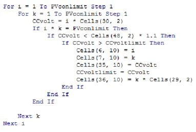
The macro reads the inputs that the user has inserted into the model, which are mainly the load, location and the specifications for the PV and battery. The optimization code is testing various nominal PV-module power outputs and battery capacities. The start and end value for the code is set by the estimations from Eq 1 and Eq 2. Figure 13 depicts an image of the optimization section of the code that has been developed in Visual Basics and then inserted as a macro in MS excel
Figure 13 Optimization code.
Where in the code, n represent the PV size and b represent the battery capacity. The optimization code tries various combinations of PV sizes and battery capacity. The first for-loop test different PV sizes and the second for-for-loop test different battery capacities. If the PV and battery combination is above the reliability limit which is controlled in the first
if-statement, the code continues to the next if-statement. The second if-statement controls if the price for the PV and battery combination is cheaper than the previous combination. If the tested PV and battery combination pass the second if-statement the code save these values and continue to test the next combination of PV and battery until both for loops reach their limits.
When the optimization is complete, the optimal PV and battery capacity will be rounded up to match the specifications of a specific battery and PV model that the user has chosen. The battery will be sized 5% higher in order keep a higher reliability since the capacity wears out (Woodbank Communications Ltd, 2016). The rounded up result are compared with the optimal result in order to see if the system is oversized.
The next step of the optimization is to find the optimal connections for the solar modules and batteries (if more than one). The macro will try all possible series and parallel combinations and will pick as many PV modules as possible in series without exceeding the charge control open circuit voltage limit (𝐶𝐶𝑣𝑜𝑐) from the specifications of the charge controller brand the
user have chosen.
The reason for this is that the current will increase equal times the amount of modules in parallel and will cause higher power losses in the cables. This means that larger and more
expensive cables are required to maintain a low power transfer loss. The voltage is equal to the amount of modules in series and higher voltages do not cause power losses in cables. The constraint can be seen in Eq 29. The maximum voltage limit of the charge controller have to be above the maximum possible open circuit voltage of the PV modules (Ministry of Mines and Energy, 2012). The voltage increases as the operating temperature decrease and therefore, the maximum possible voltage of the PV modules is set 10% higher for safety reasons (this would be set higher for climates with larger annual temperature variations).
𝑪𝑪𝒗𝒐𝒄 ≤ ∑ 𝑷𝑽𝒗𝒐𝒄 ∗ 𝟏. 𝟏 Eq 29
The code test different connection combinations in order to find the optimal one. The amount of PV’s in series is represented as i in the code and the amount of PV’s in parallel is represented as k in the code. The first and second for-loop tests all possible connection combinations for the amount of panels that the optimization code calculated. When the voltage of the PV’s in series does not exceed the charge controller (CC) voltage limit and when the amount of PV’s in series and parallel is equal to the amount of PVs that that the
optimization model calculated, the model saves that combination. A screenshot of this section of the code is shown in Figure 14.
Figure 14 Code for parallel and series combination for PV
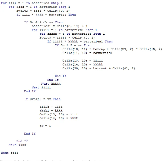
The connections of the batteries works in a similar way with increased voltage when connected in series and increased current and capacity (Ah) when connected in parallel (Ministry of Mines and Energy, 2012). A difference is that the battery bus voltage has to match the system voltage of 12, 24 or 48 which are common voltages by which charge controller and inverter are designed (NAMREP, 2006). The user can type in the system voltage they require and the code will give two optimal results, one based on what the user have typed in and another which is what the program recommends. The first optimal result is calculated by trying all combinations of battery setups for the system voltage that the user have chosen while the recommended result is trying all combinations with all battery bus
where the cables for a 12 or 24 volt system would become too large. For example, if the number of batteries from the optimization is four 12 volt batteries and the user picked 12 volt as their system voltage, the result would be one battery in series and four in parallel while the recommended result would equal two in series and two in parallel with a 24 volt system voltage. The user can choose the days of autonomy of the system. If the user would chose seven days of autonomy, the program will include seven days without any solar radiation into the radiation data.
The following section of the code Figure 15 calculates the battery setup depending on the system voltage that the user has chosen. In this code iiii represent the amount of batteries in series and kkkk represent the amount of batteries in parallel. The first two for loops test all possible combinations for the amount of batteries that the optimization code calculated. If the code finds a combination that have a battery bus voltage equal to the inserted system voltage the code saves that combination and then continue with the for loop. The second if-statement adds a battery if no combination could get a battery bus voltage that is equal to the system voltage. Then the code will test all combinations again but this time with an
Figure 15 Code for parallel and series combination for batteries.
When the optimal PV and battery connections have been found, the program will calculate the cable sizes using Eq 28. The model will round up the results to a cable size commonly available at the service providers ranging from 1.5 to 50 mm2 (Chiguvare, 2015).
The maximum current of the charge controller is calculated from the short circuit current of the solar modules in parallel or the maximum current of the batteries, depending on which one is the highest. The minimum recommended current limit is set to 25% higher for safety reasons due to surge currents which might occur at the moment an electrical appliance is turned on (Bas, 2010).
The inverter voltage has to match the system voltage of 12, 24 or 48 volts. The maximum power of the inverter is calculated from Eq 30.
The maximum load of the household is set 100 % higher for safety reasons due to surge currents and 𝜂𝑖𝑛𝑣𝑒𝑟𝑡𝑒𝑟 is the inverter efficiency (NAMREP, 2006).
3.2.9 Interface macros
The model is constructed with several macros that will make the model more user-friendly. These macros make it possible to save, change, delete and insert new PV/Battery models. The user could save the specifications for the PV/Battery that they use most frequently in order to save time. These macros are developed in a way where the user only needs to press a button in order to activate one of these macros. The macro calculates the amount of PV models that are saved in the model and place the specification for the new PV module on a free row. The model is also developed with a quotation macro which makes it possible for the user to create a quotation or invoice. The macro works in a way where the user can press on the quotation button and all important data such as the load equipment, PV and battery sizes is
automatically inserted.
3.3 MS Excel model overview
The model consists of three sections, inputs, results and errors and warnings. A user manual will be included in the model so that the user will have instructions easy accesible. All
worksheets where the calculations are made are hidden and locked. An image of the main page is depicted in Figure 16.
Figure 16 Image of the main page of the MS Excel tool.
There is two additional pages in the model accessible via the buttons located below the start button, one is a link to instructions, similar to what is described in this section and the other link is to a quotation template where inputs and results is automatically transferred.
3.3.1 Inputs
The inputs required by the model are: the electric load, specifications of the PV-module, battery and charge controller which are commonly listed on each component. All input boxes are colored in blue. First step is to insert the azimuth angle which always should be oriented to the north if possible since it equals the highest power output. Then, one of the three zones in Namibia is chosen using the drop down list.
Next step is the household load, the amount of, power and the amount of hours of usage for the equipment have to be estimated. First a load profile has to be chosen from a drop down list. Option 1 equals a standard day with peaks in the morning, lunch and evening, option 2 equals a higher load 0600-1800 in the day and option 3 equals a higher load 1600-0300 in the evening and night. An image of the load inputs is depicted in Figure 17.
Figure 17 Load inputs.
An approximate estimation is calculated from the load and can be found in Figure 18. This estimated system size will give a figure of how big the system will be and the choice of PV-module and battery model can be made from it. Note that the battery capacity is calculated in ampere hours and depends on the system voltage and the battery capacity. The approximated estimation for the battery will change if the system voltage, battery capacity or days of
autonomy is changed in the battery specifications.
Figure 18 Approximate estimation for PV and battery.
Next step is the specifications of the PV-module that will be used. The required specifications can be found in Figure 19. If the PV efficiency at STC is not listed it can be calculated with Eq 31.
𝜼𝒑𝒗=
𝑷𝑺𝑻𝑪 𝑳 ∗ 𝑯 ∗ 𝟏𝟎𝟎𝟎
Eq 31 Where L and H are the module length and height, 1000 is solar radiation during STC (W/m2) and 𝑃𝑆𝑇𝐶 is the nominal power output. The model specifications for a certain module can be saved for later use by clicking the button “Save”, the PV model will then appear in the drop down list. It is also possible to delete and edit specifications for a PV-module that is already
Figure 19 PV specifications.
Next the specification for the battery has to be inserted. The days of autonomy is the amount of time the batteries can provide power without any electricity generation of the PV-modules. A drop down list ranging from one to seven days of autonomy is available. There is an option to simulate a low reliability of 95% for a system with one day of autonomy, the rest of the options is simulating with a 99.9% reliability. A drop down list is also available and used in the same way as the PV module specifications. This can be seen in Figure 20.
Figure 20 Battery specifications.
The next step is the charge controller inputs, where SOC limit and maximum open circuit voltage have to be inserted. The lower state of charge limit is commonly set to 50% according to the code of practice. The open circuit voltage limit is the maximum voltage that the charge controller can handle. This will have an impact on how the PV modules will be connected (parallel and series) (Ministry of Mines and Energy, 2012).
The last input is the length for the cables between each component. The standard is 10-15 meters between the PV module and the charge controller, 1-1.5 meters between the charge controller and the battery and 1-15 meters between the battery and the inverter (NAMREP, 2006). When all inputs have been filled, the optimization is activated by clicking on the button “Press to start”, note that larger systems will require more execution time.
3.3.2 Results
The results are presented in three sections. The main results show the parameters for each component required for sizing and installing the system. The optimal result shows the size of
the battery and PV module without being rounded up to match the size in the specification inputs. It also shows the optimal battery connection and how oversized the system is
compared to the optimal. Other results show various parameters that are not required for the installation but still are important output. Examples are the estimated battery life span, system reliability and average daily DOD. All results are in green color and an example of results can be seen in Figure 21.
Figure 21 Results for PV and battery.
There is also an option to create a quotation based on the results and inputs by clicking on the quotation button. The amount of batteries, PV modules and a load estimation is automatically added while VAT, company names and other equipment’s costs have to be added manually. Note that the design tilt is negative since the model is designed for the PV to face south, the optimum tilt for Namibia is when the PV is facing north which is the opposite direction of the azimuth angle at 0o.
3.3.3 Errors and warnings
If the program is unable to find any optimal solution, the optimization might have to be run again with another battery or PV model. Warnings mean that the system is working but is not optimal while errors mean that the optimization have to be remade. An example can be seen in Figure 22.