Using ReSET Model to Estimate the Evapotranspiration of the
Irri-gated Crops in the South Platte River Basin, Colorado
Ahmed A. Eldeiry1
Department of Civil and Environmental Engineering, Colorado State University Reagan M. Waskom
Colorado Water Institute and CSU Water Center, Colorado State University Ayman Elhaddad
Department of Civil and Environmental Engineering, Colorado State University
Abstract. The approach presented in this study uses information derived from remote sensing to estimate (ET) as a residual from the surface energy balance equation. The objectives of this study are: 1) estimate the ET of the different irrigated crops in the South Platte River Basin; 2) compare the irrigated areas and the consumption use for the years 2001 and 2010; and 3) inves-tigate the impact of irrigation system (flood/sprinkler) on the estimated ET. 54 Landsat 5/7 sat-ellite images that cover the study area for the growing season of 2001 and 2010 were acquired and processed. In addition, the metrological data were collected from the Northern Colorado Water Conservancy District (NCWCD) on hourly and daily basis. The results of this study show that the irrigated area slightly decreased from 368,474 ha in 2001 to 344,204 in 2010, however, the flood area decreased to 56.6% and the sprinkler area increased to 43.4%. The es-timated ET using the ReSET model for the year 2001 was 2,032,610 AF with 66.1% flood and 33.9% sprinkler. However, estimated ET for the year 2010 was 1,887,945 AF with 54.6% flood and 45.4% sprinkler. The average AF/A for all irrigated area for 2001 was 2.23 with 2.18 for flood and 2.34 for sprinkler, while the average AF/A for all irrigated area for 2010 was 2.22 with 2.14 for the flood and 2.32 for the sprinkler. The errors of the estimated seasonal ET val-ues using the ReSET model compared to the reference ET of the metrological stations were less than 0.05.
1. Introduction
Water resources management is important to secure agricultural production in order to face the daunting challenges from the population growth with the existing limited re-sources of water. Evapotranspiration (ET) is the largest user of irrigation water and ac-curacy in ET estimation can be very valuable for better irrigation management. Quanti-fying the consumption of water over large areas and within irrigated projects is im-portant for water rights management, water resources planning, hydrologic water bal-ances, and water regulation (Allen et al. 2007 b). Remote sensing data are means of ob-taining consistent and frequent observation of spectral reflectance and emittance of ra-diation of the land surface on micro to macro scale (Bastiaanssen et al. 1998 a). Remote sensing has advantages over the traditional methods in estimating ET in capturing the spatial variability and provide regional estimates of ET at low cost. Remote sensing-based ET algorithms developed in recent years fill an existing gap: they are well suited for estimating crop water use or ET (Allen et al., 2007) and the spatial trends over time. Remote sensing technology holds great promise (Jha and Chowdary, 2006) as it can cost-effectively provide frequent data on a relatively large scale that allow specific wa-ter resource situations to be monitored on a long-wa-term basis.
1 Integrated Decision Support Group, Department of Civil and Environmental Engineering, Colorado State Universi-ty, 80523, Phone: (970) 491-7620, FAX: (970) 491-7626, E-Mail: aeldeiry@rams.colostate.edu
Remote sensing based technique is using surface energy balance (SEB) that can es-timate ET with a high level of spatial resolution. SEB algorithms are based on the ra-tionale that ET represents a change in the state of water, from liquid to gas, by a pro-cess that requires available energy in the environment for the vaporization of water (Su et al. 2005). There are several SEB models in the literature (Gowda et al. 2008) which mainly differ on how sensible heat flux (H) is calculated. SEB algorithm for land (SE-BAL) (Bastiaanssen et al. 1998a) uses hot and cold pixels within each satellite image to develop an empirical temperature difference equation, however, SEB index (Menenti and Choudhury 1993) is based on the contrast between wet and dry areas. Elhaddad and Garcia (2008) proposed a methodology to incorporate multiple metrological stations in-to a SEB model called remote sensing of ET (ReSET) in order in-to address the variable metrological conditions per location encountered by the remote sensing platform’s cov-erage area at the time of overpass. The use of single metrological stations does not ac-curately represent metrological conditions such as those created by topographic and/or microclimatic conditions within the coverage of a satellite scene. ReSET is a SEB model built on the same theoretical basis of its two predecessors: mapping evapotran-spiration at high resolution with internalized calibration (METRIC) (Allen et al. 2007a, b) and surface energy balance algorithm for land (SEBAL) (Bastiaanssen et al. 1998 a, b). ReSET can be used in both the calibrated and the uncalibrated modes. The calibrat-ed mode is similar to METRIC in which the reference ET from metrological stations is used to set the maximum ET value in the processed area, while in the uncalibrated mode, the model follows a similar procedure as SEBAL where no maximum ET value is imposed. ReSET has additional ability to handle data from multiple metrological sta-tions.
Traditionally, ET from agricultural fields has been estimated by multiplying a met-rological-based reference ET by a crop coefficient (Kc) determined according to the crop type and growth stage. However, there are typically some questions regarding the actual vegetative and growing conditions compared with the conditions represented by the idealized Kc values. In addition, it is difficult to predict the correct crop growth stage dates for large populations of crops and fields (Allen et al. 2007 b). In the mean-time, most conventional methods in estimating ET are based on point measurements that limit their ability to capture the spatial variability in a study area. ET varies spatial-ly and seasonalspatial-ly according to metrological and vegetation cover conditions (Hanson 1991). Hydrological models are advanced tools that are better suited to estimate the evaporation and the related hydrological processes at the regional scale (Beven et al., 1988). They have an advantage in simulating the effects of man-induced scenarios on regional hydrology. However, they need considerable expertise and extensive field data to make proper model simulations and implementation. The main contribution of this study is that it uses remote sensing approach in estimating ET that takes into considera-tion the spatial variability of the ET. It incorporates multiple metrological staconsidera-tions that can represent the metrological changes over the whole study area. In addition, using remote sensing data is costly effective and can save a lot of time and fieldwork.
2. Materials and Methods
2.1. The Study Area
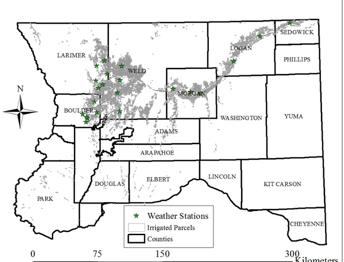
Figure 1 shows the South Platte River Basin, the metrological stations, and the irri-gated parcels in the basin. The South Platte River is one of the two principal tributaries of the Platte River, located in Colorado and Nebraska with a length of 707 (km). The river serves as the primary water supply for the Denver metro area and is the principal
source of water for the eastern Colorado. It flows north through central Denver, which was founded along its banks and its confluence with Cherry Creek. North of Denver, it flows through the agriculture heartland of northeast Colorad, directly past of the com-munities of Brighton and Fort Lupton. East of Greely, it turns eastward flowing across the Colorado Eastern Plains, past Fort Morgan and Brush. The river turns northward and continues past Sterling, and turns into Nebraska where it joins the North Platte River.
Figure 1. The South Platte River Basin, the irrigated parcels, and the metrological stations around the
South Platte River around the river.
Figure 1 shows the metrological stations scattered around the South Platte River Basin. The metrological data were collected from the Northern Colorado Water Con-servancy District (NCWCD). The alfalfa reference ET of these metrological stations is calculated using the American Society of Civil Engineers (ASCE) standardized Pen-man-Montieth equation on an hourly basis and summed for the day (midnight to mid-night). This method has been approved by the U.S. Supreme Court as the method of de-termining ET for compact compliance (Allen et al., 2005). The instantaneous and daily alfalfa reference ET, and daily wind run were considered for the processing of the Re-SET model.
2.2. Acquiring Landsat 5/7 Images
The study area is covered by three scenes of the following paths/rows (32/32, 33/32, and 33/33). 54 Landsat 5/7 images for the growing season of the 2001 and 2010
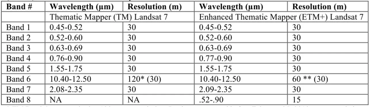
that cover the study area were acquired for the processing of the ReSET model. Landsat 5/7 scans the entire earth’s surface with an altitude of 705 kilometers +/- 5 kilometers and takes 232 orbits. This means that the satellite scans the same areas every 16 days. Table 1 shows the description of the Thematic Mapper (TM) Landsat 5 and the En-hanced Thematic Mapper (ETM+) Landsat 7 used in this study. Landsat Thematic Mapper (TM) images consist of seven spectral bands with a spatial resolution of 30 ters for Bands 1 to 5 and 7. Spatial resolution for Band 6 (thermal infrared) is 120 me-ters, but is resampled to 30-meter pixels. Approximate scene size is 170 km north-south by 183. Landsat Enhanced Thematic Mapper Plus (ETM+) images consist of eight spectral bands with a spatial resolution of 30 meters for Bands 1 to 7. The resolution for Band 8 (panchromatic) is 15 meters. All bands can collect one of two gain settings (high or low) for increased radiometric sensitivity and dynamic range, while Band 6 collects both high and low gain for all scenes. Approximate scene size is 170 km north-south by 183 km east-west.
Table 1. Description of the Thematic Mapper (TM) Landsat 5 and the Enhanced Thematic Mapper
(ETM+) Landsat 7 used in this study.
Band # Wavelength (µm) Resolution (m) Wavelength (µm) Resolution (m)
Thematic Mapper (TM) Landsat 7 Enhanced Thematic Mapper (ETM+) Landsat 7
Band 1 0.45-0.52 30 0.45-0.52 30 Band 2 0.52-0.60 30 0.52-0.60 30 Band 3 0.63-0.69 30 0.63-0.69 30 Band 4 0.76-0.90 30 0.77-0.90 30 Band 5 1.55-1.75 30 1.55-1.75 30 Band 6 10.40-12.50 120* (30) 10.40-12.50 60 ** (30) Band 7 2.08-2.35 30 2.09-2.35 30 Band 8 NA NA .52-.90 15
* TM Band 6 was acquired at 120-meter resolution. Products processed before February 25, 2010 are resampled to 60-meter pixels and after February 25, 2010 to 30-meter pixels.
* ETM+ Band 6 was acquired at 60-meter resolution. Products processed after February 25, 2010 are resampled to 30-meter pixels.
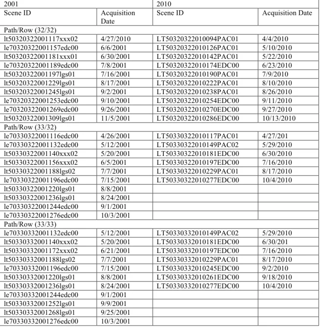
Table 2 shows the Scene ID and acquisition date of the Thematic Mapper (TM) Landsat 5 and the Enhanced Thematic Mapper (ETM+) Landsat 7 used in this study. Sometimes it is hard to find images at the same days of the starting date of the season, May 1st and the end of the season September 30th. Therefore, the first available images before the start and after the end of the growing season are collected, then while the in-terpolation to generate seasonal ET, the start and the end of the season are set to May 1st and September 30th respectively. There is no Landsat 7 in the year 2010 because on May 3rd 2003 Landsat 7’ scan line corrector failed. Therefore, the resulting images have gaps that look like lines across the images which can affect the accuracy of the results. The time intervals between either Landsat 5 or Landsat 7 is 16 days. However, when the gap is more than 16 days, it means that some images were not considered because of the clouds. The first and the last images should be free of cloud and in the case when it is hard to find a free cloud image, a raster is created with constant value of ET with 0.3 to represent either the beginning or the end of the season.
Table 2. the Thematic Mapper (TM) Landsat 5 and the Enhanced Thematic Mapper (ETM+) Landsat 7
used in this study.
2001 2010
Scene ID Acquisition
Date
Scene ID Acquisition Date
Path/Row (32/32) lt50320322001117xxx02 4/27/2010 LT50320322010094PAC01 4/4/2010 le70320322001157edc00 6/6/2001 LT50320322010126PAC01 5/10/2010 lt50320322001181xxx01 6/30/2001 LT50320322010142PAC01 5/22/2010 le70320322001189edc00 7/8/2001 LT50320322010174EDC00 6/23/2010 lt50320322001197lgs01 7/16/2001 LT50320322010190PAC01 7/9/2010 lt50320322001229lgs01 8/17/2001 LT50320322010222PAC01 8/10/2010 lt50320322001245lgs01 9/2/2001 LT50320322010238PAC01 8/26/2010 le70320322001253edc00 9/10/2001 LT50320322010254EDC00 9/11/2010 le70320322001269edc00 9/26/2001 LT50320322010270EDC00 9/27/2010 lt50320322001309lgs01 11/5/2001 LT50320322010286EDC00 10/13/2010 Path/Row (33/32) le70330322001116edc00 4/26/2001 LT50330322010117PAC01 4/27/201 le70330322001132edc00 5/12/2001 LT50330322010149PAC02 5/29/2010 lt50330322001140xxx02 5/20/2001 LT50330322010181EDC00 6/30/2010 lt50330322001156xxx02 6/5/2001 LT50330322010197EDC00 7/16/2010 lt50330322001188lgs02 7/7/2001 LT50330322010229PAC01 8/17/2010 le70330322001196edc00 7/15/2001 LT50330322010277EDC00 10/4/2010 lt50330322001220lgs01 8/8/2001 lt50330322001236lgs01 8/24/2001 le70330322001244edc00 9/1/2001 le70330322001276edc00 10/3/2001 Path/Row (33/33) le70330332001132edc00 5/12/2001 LT50330332010149PAC02 5/29/2010 lt50330332001140xxx02 5/20/2001 LT50330332010181EDC00 6/30/201 lt50330332001172xxx02 6/21/2001 LT50330332010197EDC00 7/16/2010 lt50330332001188lgs02 7/7/2001 LT50330332010229PAC01 8/17/2010 le70330332001196edc00 7/15/2001 LT50330332010245EDC00 9/2/2010 lt50330332001220lgs01 8/8/2001 LT50330332010261EDC00 9/18/2010 lt50330332001236lgs01 8/24/2001 LT50330332010277EDC00 10/4/2010 le70330332001244edc00 9/1/2001 lt50330332001252lgs01 9/9/2001 lt50330332001268lgs01 9/25/2001 le70330332001276edc00 10/3/2001
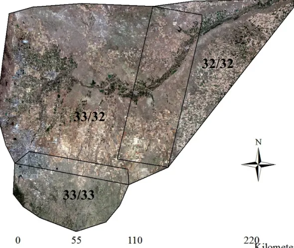
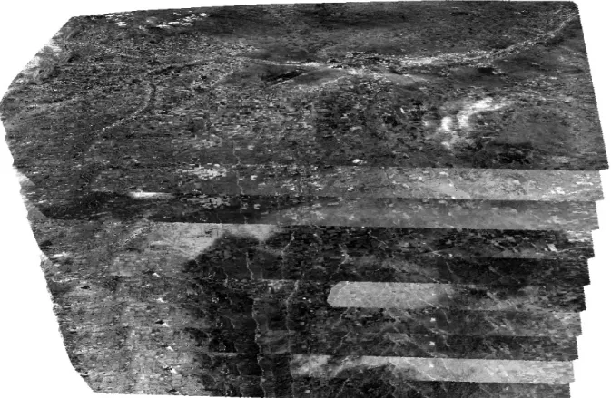
Figure 2 shows an example of three subsets of images with paths/rows 32/32, 33/32, and 33/33 that cover the study area. A boundary was created for each scene that contains the irrigated fields in that scene, and then a subset of each of the individual scenes shown in Table 2 was created by clipping that scene over the corresponding boundary shown in Figure 2. The ReSET model was applied to each subset of the indi-vidual scenes to generate a predicted ET for that day. After generating ET for each dividual image, all the images of the whole season of a specific path and row were in-terpolated to generate a seasonal ET for the irrigated fields in the scene. The final three seasonal estimated rasters were then mosaicked to generate ET for the whole study ar-ea. There are some grass pasture fields with a percentage of 1.69% of the total area on the west side of the study area not covered by these three scenes. The scenes that cover these fields are in the mountain area and often covered by cloud, which makes it im-possible to apply the models on these images. Therefore, the average value of ET of the grass pasture fields that contains within the three scenes 32/32, 33/32, and 33/33 was applied to the fields in the mountain area.
32/32
33/32
33/33
Figure 2. The subsets of the three scenes 32/32, 33/32, and 33/33 that cover the study area.
2.3. Cloud Cover
Clouds can affect the calculations of the estimated ET when using remote sensing. One of the key points in surface energy balance models calculations is assessing some cold points in well irrigated fields and some hot points in fallow or dry fields. The ex-istence of clouds, even a thin layer, will produce an error in the calculations since the areas covered by clouds will be reflected as cold areas. These areas would be misclassi-fied as actively growing areas with high ET values. Therefore, the Landsat 5/7 images were selected in a way that cloud cover does not affect the study area or the irrigated fields. In cases where fields had cloud cover, a cloud mask was created to eliminate those areas that were covered by clouds or cloud shadows. When interpolating the im-ages for the entire season, the masked areas are represented by no data. Therefore, these masked areas will be skipped in the interpolation processing for the specific image.
2.4. Applying ReSET Model
The approach presented in this study used a surface energy balance (SEB) based model (Remote Sensing of ET -ReSET) calibrated using metrological stations data. Several researchers have successfully applied SEB to estimate vegetation ET. The SEB approach requires solving the energy balance equation at the surface where the actual
ET is calculated as the residuals of the difference between the net radiation to the sur-face and the losses due to the sensible heat flux and ground heat flux. ReSET is an hanced ET estimation model based on the methodology implemented in the surface en-ergy balance algorithm for land (SEBAL) (Bastiaanssen et al. 1998a, b) and METRIC (Alen et. al. 2007 a, b). METRIC allows the user to estimate ET using data from only one metrological station; however, ReSET expands upon METRIC and takes into con-sideration the spatial variability in the parameters over a region by using data from multiple metrological stations. Therefore, ReSET can be used in estimating ET at large scale, such as the regions or river basin scales.
The ReSET model is applied in this research to estimate the ET of irrigated crops for the entire South Platte River Basin using several Landsat 5/7 scenes for the years 2001 and 2010. Each image was processed separately to generate ET for the irrigated crops. ET is computed for each pixel (30 by 30 meter) in the satellite image for the in-stantaneous time and the day of the image. Once all the images for a specific season were processed individually, they are interpolated to generate an accumulated raster for the total ET for the season. To generate the accumulated raster, the start date and the end date of the interpolation was set to be May 1st and September 30th respectively. Fig-ure 3 shows an example of the generated ET rasters of the individual images for the growing season 2001 for the subsets of images at the path/row 33/32. After completing this process of seasonal interpolation for all images of the three scenes, they were mo-saicked to generate one raster for the whole season for the whole study area.
Figure 3. Example of the generated ET rasters of the individual images for the growing season 2001 for
the subsets of images at the path/row 33/32.
The approach presented in this study uses information derived from remote sensing to estimate surface properties such as albedo, leaf area index, vegetation indices, sur-face roughness, emissivity and sursur-face temperature, and estimate ET as a residual from the surface energy balance equation. Landsat 5/7 imagery contains visible bands (1, 2, 3), infrared bands (4, 5, 7), and a thermal infrared band (6). From the visible and
infra-red bands, surface albedo is derived. The normalized difference vegetation index (NDVI) is derived from bands 3 and 4, and the surface temperature is derived from the thermal infrared band (band 6). These three components are combined with the digital elevation models (DEM) and surface roughness to calculate the net radiation (Rn) based on a function developed by Bastiaanssen (2000). The soil heat flux (G) is calcu-lated empirically using albedo, NDVI, surface temperature, and sensible heat flux. The model’s algorithm computes most of the essential hydro meteorological parameters empirically from the satellite images. The surface energy balance components, the sen-sible heat flux H, is solved iteratively, and the ET is derived as the closure term of the surface energy balance equation:
H G) (R
LE= n − − (1)
where Rn= net radiant energy exchange at the earth’s surface, which is called net radiation; LE= evapotranspiration expressed as latent heat flux density; H = net sur-face-atmosphere flux of sensible heat; and G = soil heat flux density.
The approach implemented in ReSET to estimate the latent heat flux (LE) that yields the instantaneous evapotranspiration relies on selecting two locations in the study region. The first location is called the wet pixel. Water vapor at this location is assumed to be released based on the atmospheric requirement; thus, the vertical differ-ence in temperature is down to the minimum. Under such conditions, the sensible heat flux (H) goes to zero and components of the surface energy balance equation are re-duced to net radiation Rn and soil heat flux G and latent heat flux LE:
0 G) (R
LE= n − − (2)
The wet pixel represents one of the two extreme pixels used to solve the energy equation. The second extreme pixel is the dry pixel at which ET is assumed to be zero, meaning that the latent heat flux is assumed to be zero (LE = 0). This assumption makes it possible to estimate the sensible heat flux (H) at this location since it is equal to:
G R
H= n− (3)
For a wet pixel, the difference in temperature between the near surface and the air (dt) can be assumed to be zero since maximum evaporation conditions are assumed to exist. For a dry pixel, dt is calculated for an air temperature of 20°C. Using the assump-tion that dt at a wet pixel equals zero (i.e., H wet = 0), the value of H at a dry pixel can be calculated. Once the values of H are known at two extreme pixels (wet and dry), H can be calculated for the rest of the image. Models that use reference ET as a calibra-tion method place some condicalibra-tions on the seleccalibra-tion of the cold pixel. Allen et al. (2005) recommend the cold pixel be close to the metrological station (20 to 30 km) in MET-RIC model calibration. They also recommend the image should be split into several subareas and each subarea should be processed with its own hot and cold pixels when significant variations in metrological conditions exist. This solution provides better es-timates for ET than use of one reference cold and hot pixel for the whole image.
The first calculation of H is a preliminary estimate, and calculations for H must be repeated until H reaches stability. The instability is caused by the fact that air has three stability conditions (stable, unstable, and neutral). Stability conditions must be taken in-to consideration during the calculation of H since they affect the aerodynamic re-sistance to heat transport that directly affects the value of sensible heat flux (H). Once H reaches stability, the latent heat flux can be calculated using the energy balance equa-tion Eq. (1). The latent heat flux is then converted to estimate the instantaneous evapo-transpiration. Assuming that the instantaneous evapotranspiration fraction is constant
over a whole day (24 h), the instantaneous and full day evapotranspiration can be calcu-lated as follows: ) G LE/(R ETinst−fraction = n − (4)
where: Rn, G, and LE are all instantaneous, then the ET (24-h) is calculated by: )/L G (R * ET * 86,400 ET24 = inst−fraction n24 − 24 (5)
where: ET24= 24-h evapotranspiration; 86,400 = time conversion from seconds to days; Rn24= 24-h net radiation; G24 is the 24 hour soil heat flux; L = latent heat of va-porization that is used to convert the energy to mm of evaporation. L is based on the surface temperature and represents the energy needed to evaporate a unit mass of water as calculated by the following equation developed by Harrison (1963):
6 S 273.16))*10 (T * 0.00236 (2.501 L= − − (6)
where TS = surface temperature in Kelvin.
To estimate the value of H for the rest of the image pixels, the Monin-Obukhov length similarity theory is used for correcting the calculations of sensible heat flux for atmospheric stability conditions. This is achieved through an iterative process where the surface aerodynamic resistance of heat transport ( , s m−1) at the cold and hot pixels are updated after each iteration until numerical stability is reached for the aero-dynamic resistance (typically less than 5% difference between consecutive iterations of
). Once numerical stability is reached, then H is calculated for the entire image using the coefficients of the dT function and the “ ” updated values. Next, the spatially dis-tributed latent heat flux is calculated using the energy balance equation Eq.(1). Using the estimated LE grid, the instantaneous “actual” ET grid (ETinst, mm h−1) and the evaporative fraction grid are calculated. For the model in the un-calibrated mode the 24-h ET (full day) is calculated by assuming that the instantaneous evaporative frac-tion, calculated at the time of the satellite overpass, is constant over a whole day (24 h). More details on the procedure of how ET can be estimated from satellite imagery is presented in Bastiaanssen et al. (1998b), Bastiaanssen (2000), Bastiaanssen et al. (2002), Allen et al. (2005), and Tasumi et al. (2005).
2.5. Evaluating the ReSET Performance
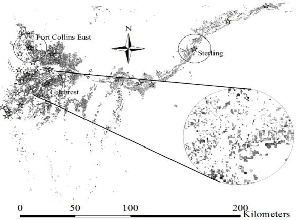
The alfalfa reference ET of the metrological station is calculated using the Ameri-can Society of Civil Engineers (ASCE) standardized Penman-Montieth equation on an hourly basis and summed for the day (midnight to midnight). This method has been ap-proved by the U.S. Supreme Court as the method of determining ET for compact com-pliance (Allen et al., 2005). Therefore, the alfalfa reference ET will be used to assess the performance of the ReSET model in estimating the ET. First, the histograms of the estimated alfalfa ET (flood/sprinkler) for the whole study area using the ReSET model will be compared with the reference ET in the study area. Second, the areas around three different metrological stations will be clipped over a circle of 20 (km) radius, and then the well-irrigated and fully-grown alfalfa areas included in that circle will be com-pared with the reference ET at that area. The criteria for selecting the metrological sta-tions are: 1) the selected station should have enough data for 2001 and 2010; 2) not at the edge in order to be surrounded by many alfalfa fields. The three stations that were selected for the evaluation are: Sterling, Fort Collins East, and Gilcrest. Figure 4 shows the circles around the Sterling, Fort Collins East, and Gilcrest stations that encompasses only alfalfa fields.
Sterling
Gilchrest Fort Collins East
Figure 4. The circles around the Sterling, Fort Collins East, and Gilcrest metrological stations that
en-compasses only alfalfa fields.
After excluding the alfalfa for each station, the zonal statistics in ArcGIS was used to the mean value of estimated ET for each individual field in the area around each sta-tion. Histograms of the means of ET of all fields around each metrological station are constructed to represent the frequency of the mean values. In the histograms, each sin-gle pixel (30 m * 30 m) in any alfalfa field is represented by a value of ET (in) and shown in the x-axes while the number of similar pixels in all alfalfa fields is shown as the frequency in the y-axis. Low values of ET are on the left side of the histogram and increases toward the right side of the histogram. This means that the fields on the right represent the well-irrigated and fully-grown alfalfa fields. However, as we getting close to the left side of the histogram, this represent the poor or stressed alfalfa fields and not fully-grown. Therefore, the alfalfa reference ET will be compared with the values at the right end tail of the histogram.
3. Results
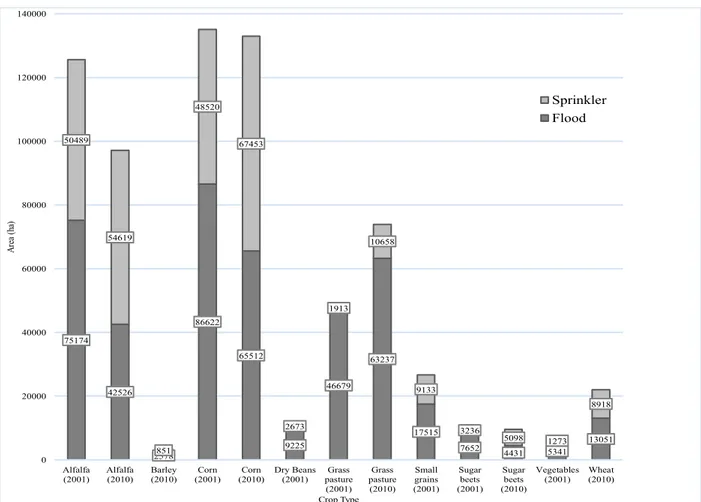
Figure 5 shows the area of irrigated crops according to irrigation system (flood/sprinkler) for the years 2001 and 2010. The small areas of less than 1% was removed from the figure to make it less crowed and make the comparison easy. However,
Table 3 shows the area of all irrigated crops in details. The total irrigated area for
2001 was 368,474 ha with 67.7% flood and 32.4% sprinkler. The irrigated area slightly decreased to 344,204 in 2010, however, the flood area decreased to 56.6% and the sprinkler area increased to 43.4%.
75174 42526 2578 86622 65512 9225 46679 63237 17515 7652 4431 5341 13051 50489 54619 851 48520 67453 2673 1913 10658 9133 3236 5098 1273 8918 0 20000 40000 60000 80000 100000 120000 140000 Alfalfa (2001) Alfalfa (2010) Barley (2010) Corn (2001) Corn (2010) Dry Beans (2001) Grass pasture (2001) Grass pasture (2010) Small grains (2001) Sugar beets (2001) Sugar beets (2010) Vegetables (2001) Wheat (2010) Ar ea (h a) Crop Type Sprinkler Flood
Figure 5. The area of irrigated crops according to irrigation system (flood/sprinkler) for the years 2001
and 2010.
Table 3. The area of irrigated crops according to irrigation system (flood/sprinkler) for the years 2001
and 2010. 2001 2010 Crop type Flood (ha) Sprinkler (ha) Total % of Total Flood (ha) Sprinkler (ha) Total (ha) % of Total Alfalfa 75,174 50,489 125,663 34.1 42,526 54,619 97,145 28.2 Barley NA NA NA 2,578 851 3,429 Bluegrass NA NA NA 878 NA 878 Corn 86,622 48,520 135,142 36.7 65,512 67,453 132,965 38.6 Dry beans 9,225 2,673 11,898 3.2 809 1,123 1,932 0.6 Grass pas-ture 46,679 1,913 48,592 13.2 63,237 10,658 73,896 21.5 Orchard 814 92 906 0.2 8 NA 8 0.0 Small grains 17,515 9,133 26,648 7.2 66 98 164 0.0 Snap beans NA NA NA 118 NA 118 0.0 Turf 70 2,053 2,123 0.6 NA 14 85 0.0 Sorghum grain NA NA NA 28 NA 28 0.0 Sugar beets 7,652 3,236 10,888 3.0 4,431 5,098 9,529 2.8 Sunflower NA NA NA 767 301 1,068 0.3 Vegetables 5,341 1,273 6,614 1.8 739 324 1,062 0.3 Wheat NA NA NA 13,051 8,918 21,969 6.4 Total 249,093 119,381 368,474 100.0 194,747 149,457 34,4204 100.0
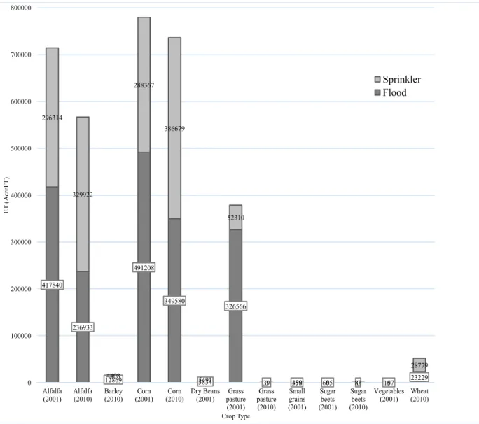
Figure 6 shows the estimated ET using the ReSET model of the irrigated crops ac-cording to irrigation system (flood/sprinkler) for the years 2001 and 2010. The crops that have estimated ET of less than 1% were removed from the figure to make it less crowed and make comparisons easier. However, Table 4 shows the ET of all irrigated
crops in detail. 417840 236933 12869 491208 349580 3834 326566 39 358 665 0 157 23229 296314 329922 4408 288367 386679 5491 52310 0 499 0 83 0 28779 0 100000 200000 300000 400000 500000 600000 700000 800000 Alfalfa
(2001) Alfalfa(2010) Barley(2010) (2001)Corn (2010)Corn Dry Beans(2001) pastureGrass (2001) Grass pasture (2010) Small grains (2001) Sugar beets (2001) Sugar beets (2010) Vegetables (2001) Wheat(2010) ET ( A cr eF T ) Crop Type Sprinkler Flood
Figure 6. The estimated ET using the ReSET model of the irrigated crops according to irrigation system
(flood/sprinkler) for the years 2001 and 2010.
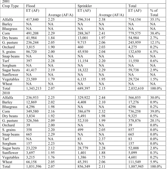
The estimated ET using the ReSET model for the year 2001 was 2,032,610 AF with 66.1% flood and 33.9% sprinkler. However, the estimated ET for the year 2010 was 1,887,945 AF with 54.6% flood and 45.4% sprinkler. In 2001 and 2010, the estimated ET for both alfalfa and corn is more than the two thirds of the total crop ET with 69.5% and 69.0% for 2001 and 2010 respectively. The average AF/A for all irrigated area for 2001 was 2.23 with 2.18 for the flood and 2.34 for the sprinkler, while the average AF/A for all irrigated area for 2010 was 2.22 with 2.14 for the flood and 2.32 for the sprinkler.
Table 4. The estimated ET using the ReSET model of the irrigated crops according to irrigation system
(flood/sprinkler) for the years 2001 and 12010. 2001
Crop Type Flood Sprinkler Total
ET (AF) Average (AF/A) ET (AF) Average (AF/A) ET (AF) % of Total Alfalfa 417,840 2.25 296,314 2.38 714,154 35.1% Barley NA NA NA NA NA NA Bluegrass NA NA NA NA NA NA Corn 491,208 2.29 288,367 2.41 779,575 38.4% Dry beans 41,984 1.84 13,001 1.97 54,984 2.7% G. pasture 236,244 2.05 9,715 2.06 245,959 12.1% Orchard 3,815 1.90 460 2.03 4,275 0.2% S. grains 86,720 2.00 45,930 2.04 132,650 6.5% Snap beans NA NA NA NA NA NA Turf 397 2.28 11,154 2.20 11,550 0.6% Sorghum NA NA NA NA NA NA Sugar beets 41,417 2.19 18,322 2.29 59,738 2.9% Sunflower NA NA NA NA NA NA Vegetables 23,589 1.79 6,135 1.95 29,724 1.5% Wheat NA NA NA NA NA NA Total 1,343,213 2.07 689,397 2.15 2,032,610 100.0% 2010 Alfalfa 236,933 2.25 329,922 2.44 566,855 30.0% Barley 12,869 2.02 4,408 2.10 17,276 0.9% Bluegrass 4,296 1.98 NA NA 4296 0.2% Corn 349,580 2.16 386,679 2.32 736,258 39.0% Dry beans 3,834 1.92 5,491 1.98 9,325 0.5% G. pasture 326,566 2.09 52,310 1.99 378,876 20.1% Orchard 39 2.00 NA NA 39 0.0% S. grains 358 2.20 499 2.05 857 0.0% Snap beans 665 2.29 NA NA 665 0.0% Turf NA NA 83 2.37 83 0.0% Sorghum 157 2.23 NA NA 157 0.0% Sugar beets 23,229 2.12 28,779 2.28 52,008 2.8% Sunflower 3,697 1.95 1,401 1.88 5,099 0.3% Vegetables 3,215 1.76 1,386 1.73 4,601 0.2% Wheat 66,158 2.05 45,391 2.06 111,549 5.9% Total 1,031,596 2.07 856,349 2.11 1,887,945 100.0%
The estimated ET for the crops with sprinkler system is higher than the estimated ET for the crops with flood system. Sprinkler system is well known for its high effi-ciency; however, the estimated ET of sprinkler is higher than that of the flood system. This can be attributed to the fact that the water application for sprinkler system is uni-form and does not go beyond the root zone area. However, the water application for flood system is non-homogeneous and goes beyond the root zone area in most cases, in addition to run off in some cases. Alfalfa and corn have the highest average ET while vegetables have the least.
0 200 400 600 800 1000 1200 1400 1600 1800 2000 9.9 11.2 12.6 14.0 15.4 16.8 18.2 19.6 21.0 22.4 23.8 25.2 26.6 27.9 29.3 30.7 32.1 33.5 34.9 36.3 Fr eq ue nc y ET(in) 0 100 200 300 400 500 600 700 800 900 1000 17. 9 19. 0 20 .1 21. 2 22. 4 23. 5 24. 6 25. 7 26 .8 27. 9 29. 0 30. 1 31. 2 32. 3 33. 5 34. 6 35. 7 36. 8 37. 9 39. 0 40. 1 Fr eq ue nc y ET(in) 0 100 200 300 400 500 600 700 800 900 15. 0 16. 2 17 .4 18. 6 19. 7 20. 9 22. 1 23. 3 24. 5 25. 6 26. 8 28. 0 29. 2 30. 3 31. 5 32. 7 33. 9 35. 1 36. 2 37. 4 Fr eq ue nc y ET(in) 0 200 400 600 800 1000 1200 1400 1600 1800 2000 10. 9 12. 3 13. 6 14. 9 16. 2 17. 5 18. 8 20. 1 21. 5 22. 8 24. 1 25. 4 26. 7 28. 0 29. 3 30. 7 32. 0 33. 3 34. 6 35. 9 37. 2 Fr eq ue nc y ET(in) 0 100 200 300 400 500 600 700 16 .0 17. 2 18. 4 19. 6 20. 8 22. 0 23. 2 24. 4 25. 6 26. 8 28. 0 29. 2 30. 4 31. 5 32. 7 33. 9 35. 1 36. 3 37. 5 38 .7 Fr eq ue nc y ET(in) 0 100 200 300 400 500 600 700 800 900 1000 10. 0 11. 4 12. 8 14. 2 15. 6 17. 0 18. 4 19. 8 21. 2 22. 6 24. 0 25. 3 26. 7 28. 1 29. 5 30. 9 32. 3 33. 7 35. 1 36 .5 Fr eq ue nc y ET(in)
Fort Collins; Ref.ET=36.5 (in)
Gilchrest; Ref.ET = 35.8 (in)
Sterling; Ref.ET = 40.7 (in) (2001)
(2001)
(2001)
Fort Collins; Ref.ET=39.1 (in)
Gilchrest; Ref.ET = 38.9 (in)
Sterling; Ref.ET = 40.3 (in) (2010)
(2010)
(2010)
Figure 7. The histograms of the estimated ET using ReSET model for all alfalfa in an area of a circle
with 20 km radius around the Fort Collins East, Gilcrest, and Sterling stations for the years 2001 and 2010.
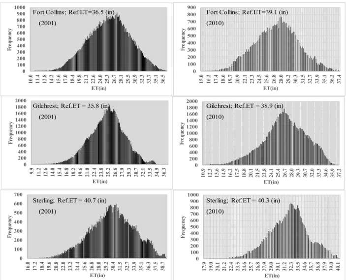
Figure 7 shows the histograms of the estimated ET using the ReSET model for all the alfalfa crops in an area of a circle with 20 km radius around the Fort Collins East, Gilcrest, and Sterling metrological stations for the years 2001 and 2010. Also, Table 5 shows the estimated ET using the ReSET model versus the reference alfalfa ET for each station.
Table 5. Comparison of the reference ET values at the stations with the ET values estimated around the
metrological stations using the NDVI*Ref.ET and ReSET models for the years 2001 and 2010.
Station Ref.ET (in) Estimated ET (in) Error %
2001 Fort Collins 36.5 36.5 0.00% Gilcrest 35.8 36.3 -‐1.39% Sterling 40.7 38.7 4.91% 2010 Fort Collins 39.1 37.4 4.35% Gilcrest 38.9 37.2 4.37% Sterling 40.3 40.1 0.50%
For the year 2001, the estimates of the ReSET model is the same of the reference ET at the Fort Collins station. The estimates of the ReSET model is very close to the refer-ence alfalfa ET at the three stations. The errors of the estimates are: 0.00%, -1.39%, and 4.91% for the Fort Collins East, Gilcrest, and Sterling metrological station respec-tively. For the year 2010, the estimates of the ReSET model for the three metrological stations are also close to to the reference alfalfa ET of the three stations. The errors of the estimates are: 4.35%, 4.37%, and 0.50% for the Fort Collins East, Gilcrest, and Sterling metrological station respectively. It is clear that the error of estimated values for both years are less than 0.05. To assess the performance of the models for the rest alfalfa, whether well-irrigated or not, we need to consider the nature of alfalfa. Similar to the rest of the irrigated crops, not all alfalfa fields in the whole study area can be irri-gated in one day. Therefore, at the time of image acquisition, some of alfalfa fields are irrigated and others are not. In the meantime, alfalfa fields are different from the other irrigated crops is a way that for any specific field after reaching the stage of full-gown, it is cut. Therefore, at the time image acquisition, some alfalfa fields are fully grown while others are not. In addition, the existence of water logging and/or high salinity spots may cause some bare spots in alfalfa fields. All of the previous can cause a distri-bution of the histogram to be close to normal distridistri-bution which is clear from Figure 7.
4. Conclusions
The approach presented in this study uses information derived from remote sensing to estimate surface properties such as albedo, leaf area index, vegetation indices, sur-face roughness, emissivity and sursur-face temperature, and estimate ET as a residual from the surface energy balance equation. ReSET model is applied in this research to esti-mate the ET of the irrigated crops of the whole basin of the South Platte River using several Landsat 5/7 scenes for the years 2001 and 2010. The ReSET model used in this study incorporates the spatial variability of wind and reference ET into the model as grids. Such an approach ensures that each cell is modeled based on its spatial location taking into consideration all the spatial variability that affects the calculation of ET. When using remote sensing data, clouds can be setback especially when it covers the area of interest. The advantage of the ReSET model is that it incorporates more than station that enables capturing the spatial variability of the weather in the study area. In addition, if there are some areas covered with cloud, these areas are masked and during the interpolation process to obtain the seasonal ET, the masked areas will be skipped. The results of this study show that the irrigated area slightly decreased in 2010. In the meantime, the flood area decreased while the sprinkler area increased from 2001 to 2010. The estimated ET for sprinkler is higher than that of flood, even though, the sprinkler is more efficient than flood. Alfalfa and corn have the highest average ET, while vegetables have the least average. The errors of the estimated ET values using the ReSET model compared to the reference ET of the metrological stations were less than 0.05.
5. References
Allen, R. G., Tasumi, M., and Trezza, R. (2005).METRIC applications manual—Version 2.0, Univ. of Idaho, Kimberly, ID.
Allen, R. G., Tasumi, M., and Trezza, R. (2007a). “Satellite-based energy balance for mapping evapo-transpiration with internalized calibration (METRIC)—Applications.”J. Irrig. Drain Eng., 133(4), 395–406.
Allen, R. G., Tasumi, M., and Trezza, R. (2007b). “Satellite-based energy balance for mapping evapo-transpiration with internalized calibration (METRIC)—Model.”J. Irrig. Drain Eng., 133(4), 380– 394.
Bastiaanssen, W. G. M. (2000). “SEBAL based sensible and latent heat fluxes in the irrigated Gedez Ba-sin, Turkey.”J. Hydrol. (Amsterdam), 229(1-2), 87–100.
Bastiaanssen, W. G. M., Ahmad, M. U. D., and Chemin, Y. (2002). “Satellite surveillance of evaporative depletion across the Indus Basin.” Water Resour. Res., 38(12), 91–99.
Bastiaanssen, W. G. M., ET al. (1998a). “Remote sensing surface energy balance algorithm for land (SEBAL): 2 Validation.” J. Hydrol. (Amsterdam), 212-213(1-4), 213–229.
Bastiaanssen, W. G. M., Menenti, M., Feddes, R. A., and Holtslag, A. A. M. (1998b).“Remote sensing surface energy balance algorithm for land (SEBAL): 1 Formulation.” J. Hydrol. (Amsterdam), 212-213(1-4), 198–212.
Beven, K.J., Wood, E.F., Sivapalan, M., 1988. On hydrological heterogeneity: catchment morphology and catchment response. J. Hydrol. 100, 353–375.
Elhaddad, A., and Garcia, L. A. (2008). “Surface energy balance-based model for estimating evapotran-spiration taking into account spatial variability in weather.” J. Irrig. Drain Eng., 134(6), 681–689. Elhaddad, A., and Garcia, L. A. (2011). “ReSET-Raster: Surface energy balance model for calculating
evapotranspiration using a raster approach.” J. Irrig. Drain Eng., 137(4), 203–210.
Gowda, P. H., Chavez, J. L., Colaizzi, P. D., Evett, S. R., Howell, T. A., and Tolk, J. A. 2008. “ET map-ping for agricultural water management: Present status and challenges.”Irrig. Sci.,26 (3), 223–237. Hanson, R. L.1991. “Evapotranspiration and droughts.” National water summary 1988–89—Hydrologic
events and floods and droughts: U.S. Geological Survey Water Supply Paper 2375, compiled by R. W. Paulson, E. B. Chase, R. S. Roberts, and D. W. Moody, USGS, Reston, Va., 99–104.
Harrison, L. P. (1963). “Fundamental concepts and definitions relating to humidity.”Chapter 3,Humidity and moisture, A. Wexler, ed., Vol. 3, Reinhold, New York, 256.
Jha M.K. and Chowdary V.M. (2006) Challenges of using remote sensing and GIS in developing nations. Hydrogeol. J. 15197–200.
Menenti, M., and Choudhury, B. J. 1993. “Parameterization of land surface evapotranspiration using a location dependent potential evapotranspiration and surface temperature range.”Proc., Exchange Processes at the Land Surface for a Range of Space and Time Scales, Vol. 212, Bolle H. J. et al., eds., IAHS Publ., Oxfordshire, U.K., 561–568.
Tasumi, M., Allen, R. G., Trezza, R., and Wright, J. L. (2005). “Satellitebased energy balance to assess with in-population variance of crop coefficient curves.”J. Irrig. Drain Eng., 131(1), 94–109. Su, H., McCabe, M. F., Wood, E. F., Su, Z., and Prueger, J. H. (2005). “Modeling evapotranspiration
during SMACEX: Comparing two approaches local- and regional-scale prediction.” J. Hydromete-or.,6 (6), 910–922.