Influences of infrastructure and attitudes to health on value of
travel time savings in bicycle journeys
Gunilla Björklund – VTI Reza Mortazavi – Dalarna University
CTS Working Paper 2013:35
Abstract
In this paper we investigate how attitudes to health and exercise in connection with cycling influence the estimation of values of travel time savings in different kinds of bicycle environments (mixed traffic, bicycle lane in the road way, bicycle path next to the road, and bicycle path not in connection with the road). The results, based on two Swedish stated choice studies, suggest that the values of travel time savings are lower when cycling in better conditions. Surprisingly, the respondents do not consider cycling on a path next to the road worse than cycling on a path not in connection to the road, indicating that they do not take traffic noise and air pollution into account in their decision to cycle. No difference can be found between cycling on a road way (mixed traffic) and cycling in a bicycle lane in the road way. The results also indicate that respondents that include health aspects in their choice to cycle have lower value of travel time savings for cycling than respondents that state that health aspects are of less importance, at least when cycling on a bicycle path. The appraisals of travel time savings regarding cycling also differ a lot depending on the respondents’ alternative travel mode. The individuals who stated that they will take the car if they do not cycle have a much higher valuation of travel time savings than the persons stating public transport as the main alternative to cycling.
Keywords: value of travel time savings; cyclists; infrastructure; attitudes; health
Centre for Transport Studies SE-100 44 Stockholm
Sweden
1
Influences of infrastructure and attitudes to health on value of travel
time savings in bicycle journeys
Gunilla Björklund1*, Reza Mortazavi2 1
Swedish National Road and Transport Research Institute (VTI) & Centre for Transport Studies
2
Dalarna University
Abstract
In this paper we investigate how attitudes to health and exercise in connection with cycling influence the estimation of values of travel time savings in different kinds of bicycle environments (mixed traffic, bicycle lane in the road way, bicycle path next to the road, and bicycle path not in connection with the road). The results, based on two Swedish stated choice studies, suggest that the values of travel time savings are lower when cycling in better conditions. Surprisingly, the respondents do not consider cycling on a path next to the road worse than cycling on a path not in connection to the road, indicating that they do not take traffic noise and air pollution into account in their decision to cycle. No difference can be found between cycling on a road way (mixed traffic) and cycling in a bicycle lane in the road way. The results also indicate that respondents that include health aspects in their choice to cycle have lower value of travel time savings for cycling than respondents that state that health aspects are of less importance, at least when cycling on a bicycle path. The appraisals of travel time savings regarding cycling also differ a lot depending on the respondents’ alternative travel mode. The individuals who stated that they will take the car if they do not cycle have a much higher valuation of travel time savings than the persons stating public transport as the main alternative to cycling.
Keywords: Value of travel time savings; cyclists; infrastructure; attitudes; health
2
1. Introduction
When planning road and rail investments, cost benefit analysis (CBA) is a common method used by authorities both to design the infrastructure and to prioritize between different
investment projects. According to Börjesson and Eliasson (2012), two possible reasons for the lack of CBA in bicycle investments are that “…the methodology is less developed for bicycle trips. Another possible reason is the implicit perception that cyclists have so low willingness to pay for time savings or other improvements that bicycle investments need to be motivated by “additional” benefits in the form of increased health, environmental effects or reduced road congestion” (p. 673). To increase the knowledge in this subject, Börjesson and Eliasson performed a study aimed at estimating valuations of different cycling facilities and at assessing the magnitude of health effects and (to a lesser extent) benefits from reduced car traffic.
The purpose of the present study is to investigate how attitudes to health and exercise in connection with cycling influence the estimation of values of travel time savings in different bicycle environments (mixed traffic, bicycle lane in the road way, bicycle path next to the road, and bicycle path not in connection with the road). The results are based on two stated choice studies carried out in four cities in Sweden. In the first study, the “handed-out” study1, the questionnaires were handed out to cyclists when they actually were cycling. In the second study, the “mailed-out” study, the questionnaires were sent home to persons in the same cities in order to receive responses from commuters, both regular cyclists and potential cyclists. The rest of the paper is organised as follows. In section 2, a brief literature review of empirical studies of travel mode choice and value of travel time savings is given. Section 3 describes the theory of valuation of travel time saving. The data collection, including a description of the questionnaire and the respondents, is presented in section 4. In section 5, the model specification is given. The results from the estimated models are then presented in section 6. Finally, section 7 concludes the paper with a discussion and conclusions.
1
3
2. Empirical studies of value of travel time savings for bicycle trips
An important element in the CBA is the value of travel time savings (VTTS). However, the research regarding cyclists’ VTTS is limited, especially regarding Swedish cyclists. The Swedish Environmental Protection Agency published in 2005 a study that laid the foundation for CBA of cycling measures in Sweden. In the absence of empirical studies of Swedish demand for bicycle trips, an indirect reasoning was made which resulted in a proposed VTTS for existing cyclists of 90 SEK/h2 in mixed traffic and 70 SEK/h on bicycle paths. Waiting time, risk exposure, and health effects were also discussed in the report. On behalf of the Swedish Transport Administration, a study was conducted by WSP (2009) where cyclists’ appraisals of travel time savings and convenience improvements were estimated based on stated preference choices. That study, which focused on cyclists in Stockholm (the capital of Sweden), gave relatively high VTTS: 159 SEK/h for cycling on street and 105 SEK/h for cycling on separate bicycle paths.
Börjesson and Eliasson (2012) made further analyses of the data by WSP (2009) which resulted in different VTTS depending on the trip time. For trips less than 40 minutes a VTTS of 176 SEK/h for cycling on street was estimated, whereas trips of 40 minutes or longer gave a value of 129 SEK/h. For cycling on a bicycle path a VTTS of 122 SEK/h was estimated for trips less than 40 minutes, and 67 SEK/h for longer trips. The mentioned values were
evaluated at the average sample income of 31,000 SEK/month.
Internationally, VTTS for cycling and choice between bicycle environments have been estimated by stated preference technique in several studies. For example, Ramjerdi et al. (2010) presented an average VTTS for cycling of 130 NOK3 per hour. In another Norwegian study, performed many years earlier, the VTTS for cycling was 59 NOK/h in a group of car drivers with cycling as alternative (Stangeby, 1997). In the same study, it was found that separated bicycle lanes was as important as more than a one hundred per cent reduction in cycle time on short trips. Hopkinson and Wardman (1996) estimated the value of a segregated bicycle path to be equal to 71 pence4. Wardman et al. (1997) estimated the VTTS for cycling in mixed traffic at 9.58 pence/minute, whereas the corresponding value on an unsegregated bicycle lane was 7.53 pence/minute and 2.87 pence/minute on a fully segregated bicycle lane.
2 The exchange rate from Swedish Kronor (SEK) to Euro (EUR) is SEK 8.34/EUR (March 30, 2013). 3 The exchange rate from Norwegian Kronor (NOK) to Euro (EUR) is NOK 7.49/EUR (March 30, 2013). 4
4
All these valuations applies for fine weather. Conditions of wind or rain and wind raised the VTTS considerably. Combining stated preference and revealed preference data, Wardman et al. (2007) estimated an overall VTTS for bicycle of 19.3 pence per minute (in 1999 prices). Separate VTTS for different bicycle environments, based on adjusted stated preference data and in pence per minute, were 19.17 for minor roads with no bicycle facilities, 19.33 for major roads with no bicycle facilities, 9.17 for non-segregated on-road bicycle lanes, 6.00 for segregated on-road bicycle lanes, and 5.50 for completely segregated bicycle ways. Tilahun et al. (2007) conducted a computer based adapted stated preference study in the U.S. in which individuals in pairwise comparisons had to choose between different bicycle environments. One of the environments was of theoretically lesser quality than the other but had always shorter travel time than the more attractive environment. Five different environments were investigated where the least attractive environment was one with no bicycle lane and on-street parking, and the most attractive one was an off-road bicycle facility. The results showed that for a given individual, keeping utility at the same level and with 20 minutes as base travel time, the off-road facility could be exchanged for 5.13 minutes of travel time, a bicycle lane for 16.41 minutes of travel time, and a no parking facility for 9.27 minutes of travel time. As argued, there exist several factors affecting the propensity to cycle. Time and cost, which are the two most important variables in travel mode choice models, are only two among others. However, in contrast to motorized travel modes cycling involves health aspects, which might influence how the individual values the time on the bicycle.
Elvik (2000) concluded in a state-of-the-art study that changes in road user health state is one of the impacts that are not yet included in the CBA and that more needs to be known about its occurrence and monetary value. Including health effects in a CBA of investments in walking and cycling track networks Sælesminde (2004) found that reduced costs related to a decrease in severe diseases and ailments constituted between two-thirds and half of the total benefit and concluded that the investments were overall highly beneficial to society. The Swedish Environmental Protection Agency (2005) concluded that individuals only to a limited extent take health effects into consideration when choosing travel mode. WSP (2007) advocated that the entire health effect of cycling should be seen as unconsidered by the individuals and that it should be treated separately by the use of WHO’s calculation sheet (see WHO, 2007).
However, Börjesson and Eliasson (2012) argue that cyclists take a large share of the health effects into account when making their travel choices and that adding health benefits to the CBA would be double-counting. They found that a) more than 60% of the responding cyclists
5
exercised less than two hours per week apart from cycling, which indicates that cycling for most respondents was their primary form of exercise, b) around 60% of the cyclists stated that they would exercise more if they cycled less or that they already exercise considerably (more than four hours per week) in other forms, and c) the bicycle VTTS for the group that stated that exercise was the most important reason to cycle (52% of the respondents) were not significantly different from the values for the group stating other reasons than exercise. It is obvious that the questions regarding health effects and CBA are not fully elucidated. In the present study we try to shed some more light on this issue.
When analysing travel mode choice with discrete choice models, researchers usually
distinguish between attributes pertaining to the various transport modes and the attributes of individuals, often called socio-economic variables. Interest has also been directed towards latent variables, i.e., variables that are not directly observable (e.g., attitudes) but instead are measured by means of indicator variables (see for example Temme et al., 2008; Vredin Johansson et al., 2006; Yáñez et al., 2010). People’s attitude to health aspects, which will be investigated in the present paper, is an example of a latent variable.
The research on how to include latent variables in the discrete choice models is still in its infancy and the two methods used – the sequential and the simultaneous approach – are still under development. Both methods have their advantages and disadvantages. The sequential approach, which means that first the latent variables are estimated and then they are included in the choice models, may cause bias in the estimates and the standard errors (Raveau et al., 2010). The second method, to estimate both processes simultaneously, has the disadvantage that it is more complex and there is currently no way to estimate more advanced models (Raveau et al., 2010). In the present paper, we use the sequential approach because we want to use an advanced model, i.e., a model that requires integration processes. To avoid the
problems with the sequential approach, we let a dummy variable measure the respondents’ attitudes to health and cycling.
3. Theory of valuation of travel time saving
The valuation of travel time saving has engaged researchers for many years. The main reason is of course that the single most important component in infrastructure projects assessments is the travellers’ gains in terms of reduced travel times. The following are important
6
contributions to the theory of value of time and value of travel time saving based on the idea that individuals maximize a utility function when making choices. Becker (1965) in a time allocation model assumed that individuals freely choose how many hours to work. His model implies that the shadow price of time is constant and equal to the wage rate and does not depend on which activity the individual is engaged in. Johnson (1966) included the work time explicitly in the utility function and showed that the value of time can be decomposed into the wage rate and the subjective valuation of time at work. Oort (1969) included even the travel time itself in the utility function which implies an additional component, the value of how time spent in the travel activity is perceived by the individual. DeSerpa (1971) and Evans (1972) assumed a technological time constraint in the sense that activities require a minimum amount of time. Individuals can reallocate time spent in one activity into another. In this sense it is meaningful to talk about value of saving time. Jara-Díaz (2003) introduced a minimum consumption constraint and argued that there is an additional component in the value of travel time savings, namely, the value of reassigned consumption.
Essentially, time can be seen as a resource and as such it has a (resource) value but it also has a value because it is required to produce and consume specific activities (commodity value of time in the words of DeSerpa, 1971). The difference between the two can be interpreted as the subjective value of saving time in an activity, e.g. travel.
3.1. A model of time allocation
Following DeSerpa (1971), Troung and Hensher (1985), and Bates (1987) a model of time allocation in a travel activity is presented here. The following assumptions are made. Individuals maximize a utility function given some constraints. Utility is derived from consuming commodities and spending time consuming them. The utility function is assumed to be twice differentiable and is maximized subject to two resource constraints; money and time. In consuming any commodity a minimum amount of time must be devoted, but there is no upper bound.
The direct utility function depends on the amount of goods and services, , that can be consumed after the cost of a trip with mode ( ) is deducted from the budget, , time devoted to the trip activity, and time available for leisure .
The money constraint that the individual faces, assuming that the entire individual’s income, , is spent on consuming goods and services, is , where is the cost of
7
the trip by mode . The time constraint is , where is the leisure time available after the trip time is deducted from the total time, , available. These two are the resource constraints. DeSerpa (1971) argued that for any specific activity there is a minimum amount of time requirement but individuals may choose to spend more time on an activity. This justifies an additional constraint: which should be seen as the time consumption constraint distinguished from the previous time resource constraint. The ’s are technological coefficients, ratio of time to cost, that may be different for different travel modes.
The Lagrangian of the problem may be written as:
( ) ( ) ( ) ( ) (1)
where is a vector of socio-economic variables. ( ) is increasing in and and is normally decreasing in . In some cases however it might be increasing in , for instance when one takes a car ride just for pleasure or a bicycle ride for relaxation and/or exercise purposes.
The first order conditions for a maximum are: , , , and ( ) . (2)
The value of time, in terms of consumption of any good, can then be defined as the ratio of the marginal utility of time to marginal utility of money:
. (3)
The first term, is the value of time as a resource (wage rate). The second term, , is the subjective value of travel time savings (VTTS). Troung and Hensher (1985) referred to this as the value of transferring time from an activity to pure leisure since time cannot be saved in the sense of being stored. Rewriting equation (3) we have:
. (4)
The subjective VTTS can then be decomposed into two parts. The first part is the resource value of time, or the opportunity cost of spending time travelling instead of doing something else. The second part is the direct value of travel time given as the ratio of marginal utility or
8
disutility (benefit or loss) of travel time to marginal utility of money. Since can be negative (normally) or positive (enjoying riding a bicycle) the subjective VTTS may be less than or greater than the resource value.
Equation (4) implies that the VTTS is different depending on the transportation mode, which normally is the result found in empirical studies. Ceteris paribus, the more unpleasant the time spent on/in a particular mode the higher will be the value of reducing that time, i.e. saving time. If for instance commuting time on a bicycle is experienced as more unpleasant than the commuting time with car then the VTTS for the mode bicycle is greater than for car.
Ceteris paribus, we would expect that the VTTS is higher for high income groups compared to low income groups because the marginal utility of money is relatively lower for them. Equation (4) also indicates that, when marginal utility of time spending cycling is positive, for instance because of a positive health effect or pure enjoyment, then ceteris paribus, the VTTS should be lower. The direct marginal utility of time spent in different activities and situations may also be relatively more negative (greater in absolute value). For instance the experience of cycling among other vehicles in the street may be more negative (less positive) than in a separated bicycle path, ceteris paribus again.
A first order Taylor approximation of the indirect utility function for individual travelling by mode is: ( ) (4)
( ) is the corner solution where the only consumption is the trip by mode . can be seen as an error term containing higher order terms and unobservable factors. Substitution of the first order conditions and the time and money constraints for a maximum gives:
( ) ( ) ( ) ( ) (5) In equation (5), the shadow price or marginal utility of money is an implicit function of income and the travel cost.
Equation (5) can be sorted out further:
9
Note that the term does not vary across alternatives in a mode choice setting and the parameter (the shadow price of time as a scarce resource) is not identified (unless the assumption that the marginal utility or disutility of travel time is zero is made which implies that ). However, since travel time varies across alternatives we can estimate the VTTS.
4. Data collection
4.1. The questionnaire
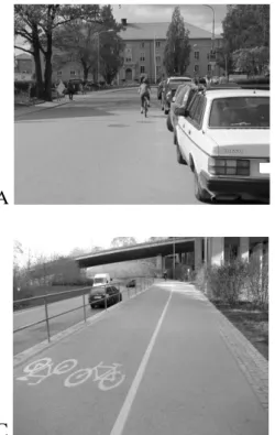
In the present study, a variant of Börjesson’s and Eliasson’s (2012) design and questionnaire is used. The main differences are that we also ask several questions about attitudes to cycling, including health and exercise, and that the stated preference-alternatives contain four different types of cycling environments instead of two. The four different environments are presented in Figure 1. Furthermore, we have a larger sample and performed the study in smaller cities. However, we do not investigate the valuation of bicycle facilities such as bicycle parking at the destination or the number of signalized intersections where the cyclists had to stop and wait.
A
C
B
D
Figure 1. Cycling environments used in the study. (A) Mixed traffic. (B) Bicycle lane in the road way. (C) Bicycle path next to the road. (D) Bicycle path not in connection with the road.
10
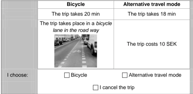
Each respondent had in twelve stated preference choices to decide whether they would have cycled or taken an alternative travel mode, where the options were car or public transport. The respondents were asked to state which of these two travel modes that would be a suitable option for them before they made their choices. To limit the number of choices for each person to twelve, three different versions of the questionnaire were constructed. In each version, three of the four bicycle environments were presented. The bicycle time consisted of the levels 20, 25, and 35 minutes, whereas the time for the alternative travel mode consisted of the levels 10, 13, and 18 minutes, and was thus always the faster mode of travel. The cost of the alternative travel mode varied between 10, 16, and 32 SEK, whereas the cost of the bicycle was assumed to be zero. Figure 2 shows an example of a stated preference choice.
Bicycle Alternative travel mode
The trip takes 20 min The trip takes 18 min The trip takes place in a bicycle
lane in the road way
The trip costs 10 SEK
I choose: Bicycle Alternative travel mode
I cancel the trip
Figure 2. An example of a stated preference choice
In addition to the stated preference choices, the questionnaire in the handed-out study included questions about the journey the respondents were performing when they got the questionnaire. Furthermore, the respondents were asked questions about factors of importance for choosing bicycle as travel mode, questions about the respondents’ travel- and exercise habits, and finally, some socio-economic questions. The questionnaire in the mailed-out study included the same stated preference choices as in the handed-out study. However, instead of asking about the respondents’ current journey we asked the respondents questions about a ordinary journey, if they had any, preferably a journey to school or work. We were only interested in regular journeys, preferably trips to work or school, because we assume that in
11
connection to these journeys people, at least in the beginning, do some conscious
considerations regarding travel times and travel costs and choice of travel mode. Only the respondents that had or could imagine themselves to take the bicycle to their destination were asked to answer the questions about cycling, including the attitude questions and the stated preference choices. The reason was that if they never had intended to cycle to their destination the questions would have been too hypothetical and far from reality for them.5
The questionnaires were tested in a small pilot study and the travel times were shortened a few minutes, resulting in the levels presented above. Before the main studies were performed, a second pilot study was conducted where questionnaires were handed out to cyclists in Stockholm, which led to some minor changes in the questionnaire (the results from the pilot study is presented in Björklund & Carlén, 2012).
4.2. Participants
Regular and potential cyclists from four Swedish cities participated in the study. The four cities were Karlstad (86,409 inhab.), Luleå (74,426 inhab.), Norrköping (130,623 inhab.), and Västerås (138,709 inhab.). In parentheses are the number of inhabitants in each municipality, valid in the end of 2011 (Statistics Sweden, 2013). These four cities were chosen because we wanted to include two middle sized cities where one had a little more developed bicycle infrastructure than the other, and two smaller cities with comparable bicycle infrastructure, but one in the north of Sweden and the other in the southern part.
In the first study, questionnaires were handed out to almost 3,000 cyclists in the four cities in June 2011. The cyclists were approached at intersections, where traffic signals or stop signs requested them to stop, or at other places where natural stops were supposed to occur. Another 838 persons declined on spot to participate in the study (some of them might have received a questionnaire already), but the others received a prepaid response envelop and the questionnaire to fill in at home. Only persons of age 18 years or older, and understanding Swedish, were recruited. Of the handed out questionnaires, 1,518 (51%) were returned and 1,250 of them were usable for the subsequent analyses in this paper. In the second study,
5 The stated preference data from the two studies is together with revealed preference data from the mailed-out
study also investigated in a study by Björklund & Isacsson (2013) with aim to forcast the impact of infrastructure on cycling behaviour.
12
1,500 questionnaires were sent home to persons between 18 and 64 years old in each of the four cities in September 2011, a total of 6,000 questionnaires. Of these, 1,848 completed questionnaires were returned, which implies a response rate of 31%. In addition, 4.5% of the questionnaires were returned due to no regular journey, wrong address, or other reason. The response rate is low, but we assume that many persons who received the questionnaire did not have any regular trip. Therefore, we can assume that the actual response rate is higher, even if we cannot say how much higher. Only the persons who had answered the stated preference choices, i.e., those who could imagine themselves to take the bicycle to their destination, and had answered the attitude questions and the socio-economic questions are included in this paper, reducing the sample size to 672 persons.
To get an indication of the reasons for non-responses in the mailed-out study, a one-page questionnaire asking about the reason not to responding in the main questionnaire was constructed. This questionnaire was sent to a random sample of 100 persons in each city among those persons who had not responded to the main questionnaire after one reminder. Of these 400 persons, a total of 72 persons (18%) returned the one-page questionnaire. The most common reason for not answering the main questionnaire was that the respondents had no ordinary trip of the kind we asked about (35% of the respondents). It is not possible to say that 35% of all non-responders did not have a trip of that kind, but we assume that it was the case for many of the persons receiving the questionnaire. This was the reason why we send out as many as 6,000 questionnaires. Also, 14% of the respondents stated that their reason for non-responding was that they had no possibility to cycle to their destination. Even if this was not a criterion, many of the questions in the questionnaire were about cycling and therefore it is reasonable that these persons did not answer the questionnaire.
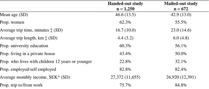
In Table 1, descriptive statistics for the demographic and socio-economic variables are presented for the handed-out study and the mailed-out study. Notably, the average trip length and trip time was a little bit longer in the mailed-out study. Also, the proportion of
respondents who made a trip to or from work was larger in the mailed-out study, which is understandable since we asked particularly about a trip to work or school. Another difference between the two samples is the proportion living with children. It might be a real difference or a result of the fact that the questions which this variable is based on were a little bit
13
Table 1. Descriptive statistics of the variables included in the choice models†
Handed-out study n = 1,250 Mailed-out study n = 672 Mean age (SD) 46.6 (13.5) 42.9 (13.0) Prop. women 62.3% 55.5%
Average trip time, minutes ‡ (SD) 16.7 (10.0) 23.0 (14.6) Average trip length, km ‡ (SD) 4.4 (3.2) 6.0 (4.8)
Prop. university education 60.3% 56.1%
Prop. living in a private house 43.4% 50.0%
Prop. who lives with children 12 years or younger 22.8% 32.1%
Prop. employed/self employed 82.8% 82.4%
Average monthly income, SEK* (SD) 27,372 (11,655) 26,920 (12,391)
Prop. trip to/from work 75.7% 84.8%
†Because of high correlation with trip time respective prop. trip to/from work, the variables trip length and prop. employed are excluded in further analyses in the paper.
‡Observed trip times and lengths which implied a speed of less than 5 km/h or more than 30 km/h are considered as unreasonable and are therefore removed. Trip times above 90 minutes are also removed.
*The participants stated their monthly before tax income, grouped into intervals of 10,000 SEK. We use the interval midpoints in the analyses. The highest interval has no upper limit and is set to 55,000 SEK/month. The lowest midpoint is 5,000 SEK/month.
5. Model specification
In a discrete choice setting with random utility maximization alternative is chosen by individual when the utility associated to that alternative is highest among all available alternatives. In this study the choice is a binary one since each choice occasion concerns choosing between bicycle, alternative and either car or buss, alternative . We can rewrite equation (6) as where can be seen as the systematic or observed part of the utility function and is the unobserved or random part. The probability of choosing the alternative, i, say bicycle, is given by:
( ) ( ) (8)
or
( ) ( ) (9)
However, as explained before each individual in our sample has made several choices in the stated choice experiment. Because of the repeated measurements over each individual the errors are no longer independent. Recognising this, random effects models are estimated.
14
These models contain a term that allows the individual-specific effects to vary and thereby accounts for differences between individuals that reflect taste heterogeneity. A modified version of the indirect utility function is then:
(10)
Here denotes the individual. is indicative of panel nature of the data where , since each individual made a minimum of one and a maximum of 12 choices.
are assumed i.i.d., ( ), and are assumed logistically distributed with mean zero and variance ⁄ , independently of . Logit models are estimated by the xtlogit command, option re, in Stata 11.0 (StataCorp, 2009) using maximum likelihood as the estimation method. To test if the panel estimator is different from the pooled estimator, the xtlogit command produces a likelihood-ratio test of , which is the proportion of the total variance contributed by the panel-level variance component: .
The empirical models that are estimated and presented in the next section are versions of the following specification based on equation (6) and (10):
∑ ∑ ∑ ( ) ∑ ( ) ∑ (11)
To simplify notations we have disregarded from the panel data dimension and the individual indexing here. Equation (11) is the indirect utility function for choosing bicycle (hence the letter b as the index here). is the alternative specific constant for bicycle. is a vector of some individual specific variables such as gender, educational level and living status and is the vector of parameters measuring the effect of these factors on utility. is a dummy
variable indicating whether the relevant alternative mode for the individual is public transport or car.
is also a dummy variable separating the participants who considered health aspects as important in their choice to take the bicycle and participants who considered health aspects as less important. In the questionnaire, the respondents were asked to state on a five-point scale (1 = No importance at all, 5 = Very large importance) how important a number of factors are in their decision to choose bicycle as travel mode. The items regarding health, safety, and flexibility/comfort were analysed in a confirmatory factor analysis with these three factors as latent variables (see Appendix). A confirmatory factor analysis tests how well some observed
15
(in this case, self-reported) variables function as indicators for an underlying, latent variable. In this paper we only use the scores for the latent variable for health. Although the latent variable is continuous, we have chosen to transform it into a dummy variable (representing high and low in attitude regarding health and cycling) because of the problems with including continuous latent variables in more advanced choice models. The health variable is based on following questions regarding exercise/health and cycling: ”A time-efficient way to exercise”, “A good way to keep weight/lose weight”, “Improves fitness”, and “Good for one’s own health”.
is a nominal variable indicating the cycling environment that was presented in the stated choice part. It has four “levels” and was described in section 4.1. Variable , measures travel time for each travel mode and variable measures the travel cost for car and public transport.
6. Results
The stated preference questions in this study concern a choice between bicycle and an
alternative travel mode. The latter turned out to be public transport for 46% of the respondents in the handed-out study and car for 54% of them. In the mailed-out study only 24% chose public transport and 76% chose car.
In the handed-out study, bicycle was chosen in 74% of all stated preference choices and car/public transport was chosen in 24% of the cases. In the rest of the cases, the respondents either marked the box stating that they cancelled the trip or marked two of the boxes. These observations were omitted in the further analyses. As many as 34% of the respondents chose bicycle in all the twelve stated preference choices, whereas only 1% chose car/public
transport in all their choices.
In the mailed-out study, bicycle was the travel mode chosen in 48% of the cases and
car/public transport were chosen in 51% of the cases. In the rest of the cases, the respondents either marked the box stating that they cancelled the trip or marked two of the boxes. Of the 672 persons analysed, 16% chose bicycle in all their choices, and 13% chose car/public transport in all their choices. Compared to the former study, the share of non-traders was almost the same, but in the former study most of the non-traders were in favour to bicycle whereas in the latter non-traders were found in both modes groups.
16
First, we estimated a simple model only including bicycle time, separated into the different environments, time for the alternative travel mode, and cost for the latter. The estimates from the logit model, titled Model 1, are presented in Table 2 (handed-out study) and Table 3 (mailed-out study).6 All coefficients are significant and have the expected signs, i.e., positive for travel time and cost for the alternative mode and negative for the bicycle travel times. Remember that the models are measuring the probability to choose bicycle. The coefficients for bicycle time on the bicycle paths are significantly smaller than the corresponding
coefficients for cycling in mixed traffic or in a bicycle lane, indicating that the respondents prefer cycling on safer paths. In the second step, we separated the travel cost for persons with income of 30,000 SEK/month or less, and persons with an income of more than 30,000 SEK/month. These models (not presented in the tables) gave a better fit both for the handed-out study and the mailed-handed-out study. When interacting the travel cost parameters with the stated alternative travel mode the models were further improved. However, it was also shown that there is a great overlap between the confidence intervals for high respectively low income for each alternative travel mode. We therefore collapsed the two income groups, getting a cost parameter only separated regarding alternative travel mode. It is obvious that people with car respectively public transport as alternative travel mode to bicycle differ in several aspects. Therefore, we estimated separate coefficients for “car drivers” respective “public travellers”7 for all time and cost coefficients, resulting in a significant improvement of the models. Next, we separated the bicycle times depending on the respondents attitudes to health and cycling (Model 2 in Table 2 and 3), improving the models considerably.
When looking at the cost coefficients it is obvious that the car drivers are less cost sensitive than the public transport travellers. There is also a tendency that the car drivers value their time outside the car more than the public travellers value the time outside their transport. The picture regarding bicycle time and attitude to health differs depending on alternative travel mode. In the handed-out study, the public travellers high in attitude to health seem to consider the time on bicycle as more pleasant than public travellers low in health attitude. This pattern is found for each type of bicycle environment. The car drivers high respective low in health attitude only differ when cycling on a bicycle path. In the mailed-out study, the opposite result
6 In Model 1 we also included dummy variables representing the different cities were the studies were
conducted. In the handed-out study none of the dummy variables were significant. In the mailed-out study there was a small difference between Luleå and Västerås, indicating that bicycle was chosen more often in Västerås than in Luleå (in the northern part of Sweden). However, we choose not to investigate this difference further.
7
17
was found, i.e., the car drivers high respective low in attitude to health differ for each type of bicycle environment, whereas the public travellers high respective low in health attitude only differ when cycling on a bicycle path.
Finally, we included the socio-economic variables and self-reported bicycle time (Model 3 in Table 2 and 3). For the handed-out study the AIC become lower and the likelihood-ratio test shows a significant improvement, whereas the BIC become higher. For the mailed-out study both the AIC, to some degree, and the BIC become higher when adding these variables but the likelihood-ratio test shows that there is a tendency to model improvement (at ten percent-level). In the handed-out study, several added variables influence the choice to take the bicycle. It is shown that older persons have a slightly larger propensity to bicycle and that higher self-reported travel time has a strong positive influence on the choice to bicycle. Persons living with children 12 years or younger tend to have a less probability to take the bicycle, and journeys to or from work have a negative influence on cycling. The added variables that have a small importance in the mailed-out study are if the respondents living in a private house and self-reported travel time, which in contrast to the handed-out study shows a small decrease in choosing the bicycle for longer trips.
18
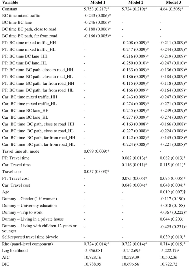
Table 2. Parameter estimates in the handed-out study (S.E.)
* Significant at 0.1% level; † Significant at 10% level.
Number of persons in all models is 1,250 and total number of observations is 14,746. BC = Bicycle, PT = Public transport, HH = Health high, HL = Health low
Variable Model 1 Model 2 Model 3
Constant 5.753 (0.217)* 5.724 (0.219)* 4.64 (0.505)* BC time mixed traffic -0.243 (0.006)* - -
BC time BC lane -0.246 (0.006)* - -
BC time BC path, close to road -0.180 (0.006)* - - BC time BC path, far from road -0.166 (0.005)* - -
PT: BC time mixed traffic_HH - -0.208 (0.009)* -0.211 (0.009)* PT: BC time mixed traffic_HL - -0.247 (0.009)* -0.244 (0.009)* PT: BC time BC lane_HH - -0.216 (0.009)* -0.219 (0.009)* PT: BC time BC lane_HL - -0.250 (0.010)* -0.247 (0.010)* PT: BC time BC path, close to road_HH - -0.133 (0.009)* -0.136 (0.009)* PT: BC time BC path, close to road_HL - -0.186 (0.009)* -0.184 (0.009)* PT: BC time BC path, far from road_HH - -0.115 (0.009)* -0.118 (0.009)* PT: BC time BC path, far from road_HL - -0.166 (0.009)* -0.164 (0.009)* Car: BC time mixed traffic_HH - -0.243 (0.009)* -0.247 (0.009)* Car: BC time mixed traffic_HL - -0.274 (0.009)* -0.271 (0.009)* Car: BC time BC lane_HH - -0.245 (0.009)* -0.249 (0.009)* Car: BC time BC lane_HL - -0.277 (0.009)* -0.274 (0.009)* Car: BC time BC path, close to road_HH - -0.163 (0.008)* -0.166 (0.008)* Car: BC time BC path, close to road_HL - -0.227 (0.008)* -0.224 (0.008)* Car: BC time BC path, far from road_HH - -0.142 (0.008)* -0.145 (0.008)* Car: BC time BC path, far from road_HL - -0.224 (0.008)* -0.221 (0.008)*
Travel time alt. mode 0.099 (0.009)* - -
PT: Travel time - 0.082 (0.013)* 0.082 (0.013)*
Car: Travel time - 0.116 (0.011)* 0.115 (0.011)*
Travel cost 0.057 (0.003)* - -
PT: Travel cost - 0.075 (0.005)* 0.075 (0.005)*
Car: Travel cost - 0.048 (0.004)* 0.048 (0.004)*
Age - - 0.019 (0.007)†
Dummy – Gender (1 if woman) - - -0.117 (0.190)
Dummy – University education - - -0.018 (0.188)
Dummy – Trip to work - - -0.367 (0.222)†
Dummy – Living in a private house - - 0.044 (0.203) Dummy – Living with children 12 years or
younger
- - -0.425 (0.231)†
Self-reported travel time bicycle - - 0.039 (0.010)* Rho (panel-level component) 0.724 (0.014)* 0.722 (0.014)* 0.714 (0.015)* Log likelihood -5,356.081 -5,242.695 -5,222.179
AIC 10,728.16 10,529.39 10,502.36
19
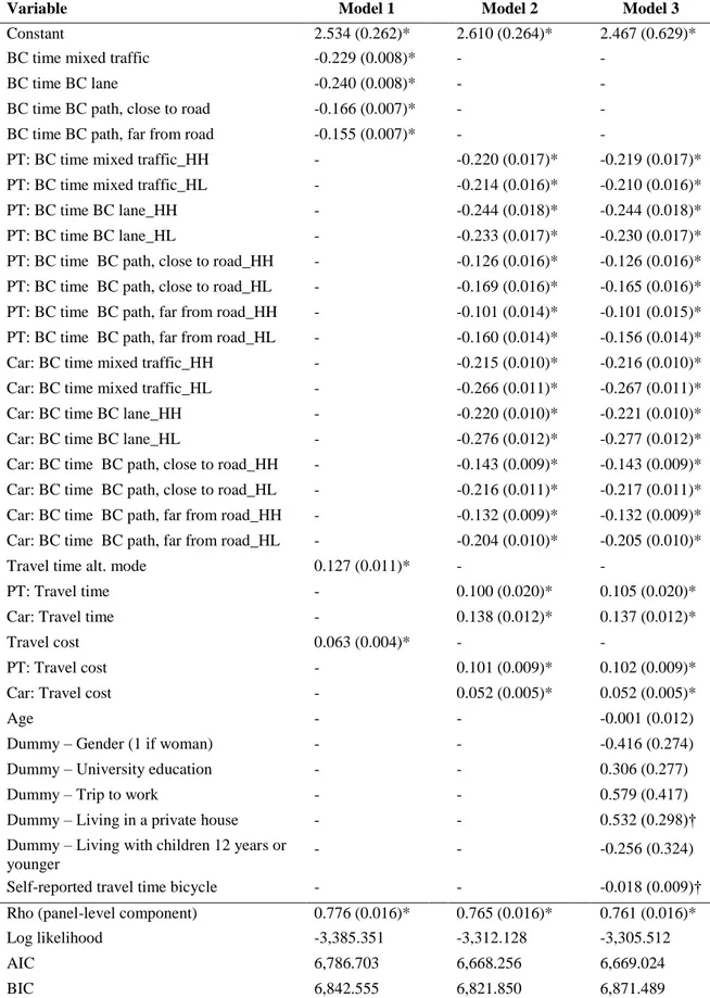
Table 3. Parameter estimates in the mailed-out study (S.E.)
* Significant at 0.1% level; † Significant at 10% level.
Number of persons in all models is 672 and total number of observations is 7,955. BC = Bicycle, PT = Public transport, HH = Health high, HL = Health low
Variable Model 1 Model 2 Model 3
Constant 2.534 (0.262)* 2.610 (0.264)* 2.467 (0.629)* BC time mixed traffic -0.229 (0.008)* - -
BC time BC lane -0.240 (0.008)* - -
BC time BC path, close to road -0.166 (0.007)* - - BC time BC path, far from road -0.155 (0.007)* - -
PT: BC time mixed traffic_HH - -0.220 (0.017)* -0.219 (0.017)* PT: BC time mixed traffic_HL - -0.214 (0.016)* -0.210 (0.016)* PT: BC time BC lane_HH - -0.244 (0.018)* -0.244 (0.018)* PT: BC time BC lane_HL - -0.233 (0.017)* -0.230 (0.017)* PT: BC time BC path, close to road_HH - -0.126 (0.016)* -0.126 (0.016)* PT: BC time BC path, close to road_HL - -0.169 (0.016)* -0.165 (0.016)* PT: BC time BC path, far from road_HH - -0.101 (0.014)* -0.101 (0.015)* PT: BC time BC path, far from road_HL - -0.160 (0.014)* -0.156 (0.014)* Car: BC time mixed traffic_HH - -0.215 (0.010)* -0.216 (0.010)* Car: BC time mixed traffic_HL - -0.266 (0.011)* -0.267 (0.011)* Car: BC time BC lane_HH - -0.220 (0.010)* -0.221 (0.010)* Car: BC time BC lane_HL - -0.276 (0.012)* -0.277 (0.012)* Car: BC time BC path, close to road_HH - -0.143 (0.009)* -0.143 (0.009)* Car: BC time BC path, close to road_HL - -0.216 (0.011)* -0.217 (0.011)* Car: BC time BC path, far from road_HH - -0.132 (0.009)* -0.132 (0.009)* Car: BC time BC path, far from road_HL - -0.204 (0.010)* -0.205 (0.010)*
Travel time alt. mode 0.127 (0.011)* - -
PT: Travel time - 0.100 (0.020)* 0.105 (0.020)*
Car: Travel time - 0.138 (0.012)* 0.137 (0.012)*
Travel cost 0.063 (0.004)* - -
PT: Travel cost - 0.101 (0.009)* 0.102 (0.009)*
Car: Travel cost - 0.052 (0.005)* 0.052 (0.005)*
Age - - -0.001 (0.012)
Dummy – Gender (1 if woman) - - -0.416 (0.274)
Dummy – University education - - 0.306 (0.277)
Dummy – Trip to work - - 0.579 (0.417)
Dummy – Living in a private house - - 0.532 (0.298)† Dummy – Living with children 12 years or
younger
- - -0.256 (0.324)
Self-reported travel time bicycle - - -0.018 (0.009)† Rho (panel-level component) 0.776 (0.016)* 0.765 (0.016)* 0.761 (0.016)* Log likelihood -3,385.351 -3,312.128 -3,305.512
AIC 6,786.703 6,668.256 6,669.024
20
In Table 4 and 5, the VTTS from the handed-out study respectively the mailed-out study are presented. We choose to base the estimates on Model 2 because that model seems most robust.
Table 4. Travel time saving values in the handed-out study (SEK/h)
Value of travel time saving n = 1,250
Infrastructure and health attitude Alt.travel mode car Alt. travel mode PT Cycle time mixed traffic
Health high 305 (253-358) 167 (142-191)
Health low 344 (286-402) 198 (171-226)
Cycle time BC path in road way
Health high 308 (254-361) 173 (148-198)
Health low 347 (289-406) 201 (172-229)
Cycle time BC path, next to road
Health high 204 (167-242) 107 (88-126)
Health low 285 (236-333) 150 (127-172)
Cycle time BC path, far from road
Health high 179 (145-213) 92 (74-110)
Health low 280 (232-329) 133 (112-154)
Alternative travel mode 145 (108-182) 66 (43-89)
PT = Public transport
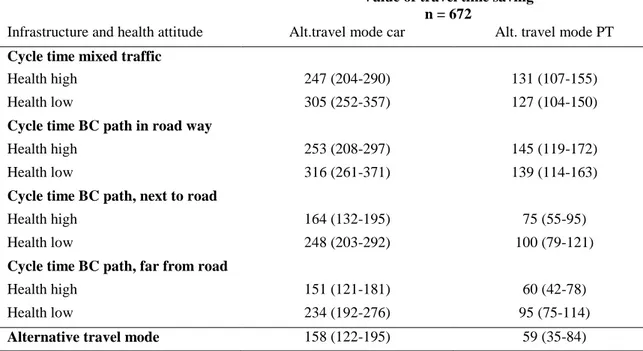
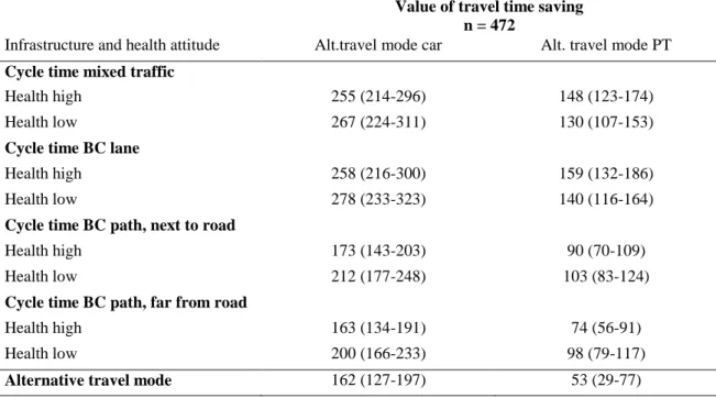
Table 5. Travel time saving values in the mailed-out study (SEK/h)
Value of travel time saving n = 672
Infrastructure and health attitude Alt.travel mode car Alt. travel mode PT Cycle time mixed traffic
Health high 247 (204-290) 131 (107-155)
Health low 305 (252-357) 127 (104-150)
Cycle time BC path in road way
Health high 253 (208-297) 145 (119-172)
Health low 316 (261-371) 139 (114-163)
Cycle time BC path, next to road
Health high 164 (132-195) 75 (55-95)
Health low 248 (203-292) 100 (79-121)
Cycle time BC path, far from road
Health high 151 (121-181) 60 (42-78)
Health low 234 (192-276) 95 (75-114)
Alternative travel mode 158 (122-195) 59 (35-84)
21
One striking result in Table 4 and 5 is that persons stating car as alternative travel mode to cycling have much higher VTTS, both when it comes to the alternative travel mode and regarding cycling, than persons stating public transport as alternative mode. One possible explanation is that the former have a higher income than the latter (handed-out study: car drivers = 29,884 SEK/month, public travellers = 24,265 SEK/month; mailed-out study: car drivers = 28,684 SEK/month, public travellers = 21,226 SEK/month). However, this is not the whole explanation because the income effect disappeared when we introduced the alternative travel mode in the models. Apparently, car drivers and public travellers differ in more aspects than income. Another notable result is the tendencies that the persons in the mailed-out study have slightly smaller values of VTTS than the persons in the handed-out study.
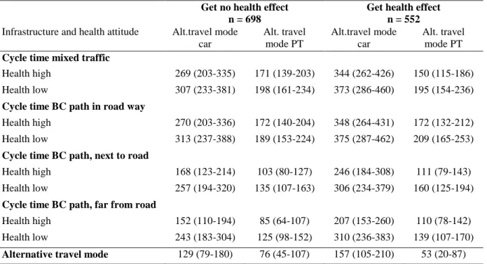
The results show that the respondents’ attitudes to health and cycling influence how they value their time on the bicycle. The respondents that are high in attitude to health seem to consider the time on the bicycle as more pleasant than respondents low in health attitude, at least when they travel on a bicycle path. This is a subjective measure of health and cycling. We are also interested in a more objective measure, i.e., if the respondents really get a health effect of their cycling. Measuring physiological changes is beyond the scope of this study, but we make an assumption that persons who state that they will not exercise more if they cycle less and exercise in other forms than cycling at a maximum of 4 hours per week get a health effect of their cycling. On the other hand, persons who stated that they actually would exercise more if they cycled less, or they do not know, and exercise in other forms than cycling at least 5 hours per week get no extra health effect of their cycling. The VTTS from these analyses are presented in Table 6 and 7, based on estimates from models including the same variables as in Model 2.
The results show that there are no large differences in VTTS between the persons who get a health effect and those who do not. However, there is a small tendency that the persons who get a health effect of their cycling have larger VTTS regarding cycling.
22
Table 6. Travel time saving values in the handed-out study, no health effect and health effect separated (SEK/h)
Get no health effect n = 698
Get health effect n = 552 Infrastructure and health attitude Alt.travel mode
car Alt. travel mode PT transport Alt.travel mode car Alt. travel mode PT transport Cycle time mixed traffic
Health high 269 (203-335) 171 (139-203) 344 (262-426) 150 (115-186) Health low 307 (233-381) 198 (161-234) 373 (286-460) 195 (154-236) Cycle time BC path in road way
Health high 270 (203-336) 172 (140-204) 348 (264-431) 172 (132-212) Health low 313 (237-388) 189 (153-224) 375 (287-462) 209 (165-253) Cycle time BC path, next to road
Health high 168 (123-214) 103 (80-127) 246 (184-308) 111 (79-143) Health low 257 (194-320) 135 (107-163) 306 (234-379) 160 (125-194) Cycle time BC path, far from road
Health high 152 (110-194) 85 (64-107) 207 (153-260) 110 (78-142) Health low 243 (183-304) 125 (98-152) 310 (236-383) 139 (107-170) Alternative travel mode 129 (79-180) 76 (45-107) 157 (105-210) 53 (20-87) PT = Public transport. Note: Separated models are estimated for the two groups.
Table 7. Travel time saving values in the mailed-out study, no health effect and health effect separated (SEK/h)
Get no health effect n = 346
Get health effect n = 326 Infrastructure and health attitude Alt.travel mode
car Alt. travel mode PT transport Alt.travel mode car Alt. travel mode PT transport Cycle time mixed traffic
Health high 229 (177-281) 126 (99-152) 268 (196-340) 143 (92-193) Health low 289 (223-356) 115 (90-139) 320 (236-404) 151 (101-200) Cycle time BC path in road way
Health high 228 (175-280) 127 (100-154) 285 (209-362) 188 (125-251) Health low 293 (226-361) 128 (102-154) 338 (250-427) 160 (107-212) Cycle time BC path, next to road
Health high 160 (120-199) 78 (56-100) 168 (118-218) 71 (33-110) Health low 237 (180-293) 93 (69-117) 258 (189-328) 114 (71-156) Cycle time BC path, far from road
Health high 139 (102-175) 59 (40-79) 168 (118-218) 65 (29-100) Health low 220 (167-272) 88 (67-110) 247 (181-313) 106 (66-146) Alternative travel mode 143 (97-190) 60 (33-87) 174 (117-232) 60 (12-107) PT = Public transport. Note: Separated models are estimated for the two groups.
23
Sensitivity analyses
Sensitivity analyses are here presented by splitting the samples into different subsamples and compare the estimated VTTS. All analyses in this section are based on estimates from models including the same variables as in Model 2.
First, we omitted all non-traders in both studies, i.e., respondents who chosen either bicycle or car/public transport in all twelve stated preference choices, before we estimated the models again. The results from this analyses (see Table A1 and A2 in Appendix) show that, with some exceptions, the VTTS including non-traders and the ones only including traders do not differ much.
In the next analysis we compare respondents who in the mailed-out study state that they take the bicycle to their destination, either the whole way or on a part of journey, at least two times a week during the summer period (April to September) and those who do not. In this way we can see if potential cyclists differ from regular bicyclists in their VTTS. The results (see Table A3 in Appendix) show that among persons stating car as their alternative travel mode there is a tendency that potential cyclists have larger VTTS than the regular cyclists, whereas the opposite are shown for the cyclists stating public transport as alternative travel mode. However, only seventeen per cent of the potential cyclists have public transport as their alternative mode and the analysis should therefore be considered with some cautiousness. Further, the confidence intervals were very wide and overlapping. The time coefficients for public transport and for cycle time on bicycle path not in connection to the road way in the public transport group were non-significant for the potential cyclists and the VTTS were therefore not calculated in these cases.
All analyses so far show that the persons who stated car as an alternative travel mode to cycling value their time different than the persons stating public transport. Therefore, in the last analysis we compare the values of bicycle travel time savings for persons who according to themselves actually cycle to their destination at least two times per week (and do not take another travel mode two times a week or more often), and persons who took the car at least two times per week (and no other travel mode two times a week or more often). This analysis is only possible to perform on the mailed-out data, because it is only in that study we asked about the actual use of different travel modes, and only for the individuals who choose car as alternative travel mode, because the public travellers were too few. The results from the analysis are presented in Table A4 in Appendix. Although there were some tendencies that the
24
car drivers had a higher VTTS for cycling than the cyclists had, none of the differences were significant. It can be noted that whereas the constant in the model for the cyclists was very large positive and significant (p < 0.001), the constant in the car drivers group was indeed positive and significant, but much smaller (p < 0.05), indicating that there exist factors not measured by the attributes included in the model that make the cyclists take the bicycle that do not exist among the car drivers, or at least exist to a smaller extent.
7. Discussion and conclusions
The results suggest that regular and potential cyclists value cycling on bicycle paths higher than they value bicycling in mixed traffic or in bicycle lanes, at least in these hypothetical situations. This cycling improvement is valued on average between 53 and 65 SEK in the group with public transport as alternative travel mode. Surprisingly, the respondents do not consider cycling on a path next to the road worse than cycling on a path not in connection to the road, indicating that they do not take traffic noise and air pollution into account in their decision to cycle. However, it is possible that aspects of unsecurity are involved when cycling on a bicycle path far from other road users, or an apprehension that bicycle paths not in connection to the road implicate longer trips. The results are in concordance with the finding by Tilahun et al. (2007) that bicycle lanes (in connection to the road) were valued higher than a completely off-road facility. We also find that the respondents do not differ between cycling on a road way and cycling in a bicycle lane in the road way. One reason can be that the respondents are not custom to bicycle lanes, which foremost exists in larger cities.
The results also indicate that respondents that include health aspects in their choice to take the bicycle have lower VTTS for cycling than respondents that state that health aspects are of less importance. The health aspects seem to have greatest effect when cycling on a bicycle path. However, one must be aware that this is one of the first attempts to separate the individual’s own appraisal of an imagined or actual health effect and the estimation of value travel time savings and there is some noise in the results. For example, because most of the respondents stated that health aspects have at least some influence in their choice to take the bicycle, it is not possible to create a group of persons that state that health aspects are of no importance at all. In this study we created a dummy variable for high respective low in attitude to health and cycling by cutting the latent continuous health variable at the median. In earlier analyses of the data from the handed-out study (Björklund & Carlén, 2012) we separated the continuous
25
variable into three pieces and created a dummy variable by including only the two extreme groups. In this way, the estimated VTTS for the group with high attitude to health became smaller and the VTTS for the group low in attitude to health became larger. However, by this procedure we lose a lot of observations which was the primary reason why we include all of the observations in the present study. Another problem is that we have no control over how the respondents perceive the questions regarding health and exercise and if they have a realistic perception about how cycling influence their health now and in the future. Further research on cycling and health effects should put great emphasis to try to sort out these issues. There was a tendency that the persons who “objectively” get a health effect by cycling have larger VTTS than the persons who do not get a health effect. It is probably so that persons who do not exercise much and should not compensate for their exercise loss if they cycled less also think it is rather unpleasant to cycle, consequently they should have higher VTTS for cycling. However, the difference between these two groups was not large enough to be
significant.
The VTTS were larger for cycling than for car or public transport, as expected. The bicycle travel time savings are valued from equal up to three times more than savings in the
alternative travel mode, depending on type of bicycle environment and health attitude, indicating that the relative VTTS are in line with the results from other studies (e.g., Börjesson & Eliasson, 2012; Ramjerdi et al., 2010; Wardman et al., 2007).
At a first glance, the VTTS for cycling in this study seem to be larger than in other studies. However, a closer look reveals that the values in this study actually do not differ much from values in the few other studies that have been done. First, we have a larger share of
individuals that gave car as their alternative travel mode than for example Börjesson & Eliasson (2012). When performing separate analyses for persons with car respective public transport it is shown that the bicycle VTTS in the public transport group are in the same range as this earlier study. Secondly, our VTTS for the alternative mode public transport are in line with the results from other studies (Börjesson & Eliasson, 2012; Ramjerdi et al., 2010; WSP, 2010) but our estimated VTTS for car trips are much higher. Thirdly, we have a large share of trips to or from work, which normally leads to higher VTTS. Fourthly, the respondents in our study had relatively short trips, which also are supposed to lead to higher VTTS.
It is clear that the appraisals of travel time savings regarding bicycle differ a lot depending on the alternative travel mode the respondents have given. The individuals with car as their main
26
alternative transportation mode have much higher VTTS than the persons stating public transport as the main alternative. This was a finding also made by Fosgerau et al. (2010). In their study car drivers had higher VTTS both in car, bus, and train, than what bus and train users had. The difference between respondents stating car respective public transport as alternative mode in the present study can to some degree be explained by a smaller income for the latter, but there are still some differences left to be explained. In an attempt to further elaborate this finding we estimated separate VTTS for actual car drivers and actual cyclists among the respondents stating car as alternative travel mode and found no differences between them, although there were some tendencies that the car drivers had a higher VTTS for cycling than the cyclists had. Another result on this theme was the tendencies by the respondents in the handed-out study to have higher VTTS than the respondents in the mailed-out study, indicating tendencies to strategic behaviour.
The lower VTTS for the public travellers suggest that potential cyclists are to be found among public transport users. Rietveld and Daniel (2004) drew the same conclusion when finding that public transport had a low share in the Netherlands whereas the bicycle share was the highest of the European countries. However, they also concluded that cycling and public transport may be complements, not only competitive transport modes.
To conclude with, it should be noted that in this study we have investigated how regular and potential cyclists value bicycle improvements such as bicycle paths. We have not investigated how such improvements and as a possible consequence a larger share of cyclists would influence safety. When planning bicycle investments advantages and disadvantages regarding safety aspects should also be considered.
Acknowledgements
The authors would like to thank the Swedish National Road Administration for funding and all the regular and potential cyclists who participated in the study. We would also like to thank the participants in different seminars where the study has been presented and all persons who in different stages in the study have provided helpful comments, especially the
colleagues at the Swedish National Road and Transport Research Institute. A special thank to professor Mark Wardman for valuable comments on the manuscript. Any remaining errors are, of course, the authors’ responsibility.
27
References
Bates, J.J. (1985) Measuring travel time values with a discrete choice model: a note. Economic Journal, 97, 493-498.
Becker, G. (1965). A theory of the allocation of time. Economic Journal, 75, 493-517.
Björklund, G. & Carlén, B. (2012). Värdering av restidsbesparingar vid cykelresor [Valuation of travel time savings in bicycle trips]. (VTI notat 26-2012). Stockholm, Sweden: Swedish National Road and Transport Research Institute.
Björklund, G. & Isacsson, G. (2013). Forecasting the impact of infrastructure on Swedish commuters’ cycling behaviour. Unpublished manuscript.
Börjesson, M. & Eliasson, J. (2012). The value of time and external benefits in bicycle appraisal. Transportation Research Part A, 46, 673–683.
DeSerpa, A. (1971). A theory of the economics of time. Economic Journal, 81, 828-846. Elvik, R. (2000). Which are the relevant costs and benefits of road safety measures designed for pedestrians and cyclists? Accident Analysis and Prevention, 32, 37-45.
Evans A. W. (1972). On the theory of the valuation and allocation of time. Scottish Journal of Political Economy, 19, 1-17.
Fosgerau, M., Hjorth, K. & Lyk-Jensen, S. V. (2010). Between-mode-differences in the value of travel time: Self-selection or strategic behaviour? Transportation Research Part D, 15, 370– 381.
Hopkinson, P. & Wardman, M. (1996). Evaluating the demand for new cycle facilities. Transport Policy, 3, 241-249.
Jara-Díaz, S. R. (2003). On the goods-activities technical relations in the time allocation theory. Transportation, 30, 245-260.
Johnson, M. B. (1966) Travel time and the price of leisure. Western Economic Journal, 4, 135-145.
Oort, C. J. (1969). The evaluation of travelling time. Journal of Transport Economics and Policy, 3, 279-286.
28
Ramjerdi, F., Flügel, S., Samstad, H. & Killi, M. (2010). Den norske verdsettingsstudien – Tid [The Norwegian valuation study – Time]. (TØI rapport 1053B/2010). Oslo, Norway: Transportøkonomisk institutt.
Raveau, S., Álvarez-Daziano, R., Yáñez, M. F., Bolduc, D., & Ortúzar, J. de D. (2010). Sequential and simultaneous estimation of hybrid discrete choice models. Transportation Research Record: Journal of the Transportation Research Board, No 2156, 131-139.
Rietveld, P. & Daniel, V. (2004). Determinants of bicycle use: do municipal policies matter? Transportation Research Part A, 38, 531-550.
Sælesminde, K. (2004). Cost-benefit analyses of walking and cycling track networks taking into account insecurity, health effects and external costs of motorized traffic. Transportation Research Part A, 38, 593-606.
Stangeby, I. (1997). Attitudes towards walking and cycling instead of using a car. (TØI report 370/1997). Oslo, Norway: Transportøkonomisk institutt.
StataCorp. (2009) Stata Statistical Software: Release 11. College Station, Tx. Statistics Sweden. (2013). Population statistics. Retrieved 26 March 2013 at http://www.scb.se/Pages/TableAndChart____308468.aspx
Swedish Environmental Protection Agency. (2005). Den samhällsekonomiska nyttan av cykeltrafikåtgärder [The social benefit of cycling measures]. Report 5456. Sweden, Stockholm: Naturvårdsverket.
Temme, D., Paulssen, M., & Dannewald, T. (2008). Incorporating latent variables into discrete choice models – A simultaneous estimation approach using SEM software. BusinessResearch, 1, 220-237.
Tilahun, N. Y., Levinson, D. M., & Krizek, K. J. (2007). Trails, lanes, or traffic: Valuing bicycle facilities with an adaptive stated preference survey. Transportation Research Part A, 41, 287–301.
Troung, T. P. & Hensher, D. (1985) Measurement of travel time values and opportunity cost from a discrete-choice model. Economic Journal, 95, 438-451.
29
Vredin Johansson, M., Heldt, T., & Johansson, P. (2006). The effects of attitudes and personality traits on mode choice. Transportation Research Part A, 40, 507-525. Wardman, M., Hatfield, R., & Page, M. (1997). The UK national cycling strategy: can improved facilities meet the targets? Transport Policy, 4, 123-133.
Wardman, M., Tight, M., & Page, M. (2007). Factors influencing the propensity to cycle to work. Transportation Research Part A, 41, 339-350.
WHO. (2007). Health economic assessment tool for cycling. Retrieved at http://www.euro.who.in/transports/policy/20070503_1
WSP. (2007). Utvecklingsplan för att möjliggöra samhällsekonomiska kalkyler av cykelåtgärder [Developing plan for facilitating social benefit-cost analyses of cycling measures]. Report 2007:15. Sweden, Stockholm: WSP Analys och Strategi.
WSP. (2009). Värdering av tid och bekvämlighet vid cykling [Valuation of time and comfort when cycling]. Report 2008:23. Sweden, Stockholm: WSP Analys och Strategi.
WSP (2010). Trafikanters värdering av tid. Den nationella tidsvärdesstudien 2007/08 [Road users’ valuation of time. The national value of time study 2007/2008]. Report 2010:11. Sweden, Stockholm: WSP Analys och Strategi.
Yáñez, M. F., Raveau, S., & Ortúzar, J. de D. (2010). Inclusion of latent variables in mixed logit models: Modelling and forecasting. Transportation Research Part A, 44, 744-753.
30
Appendix
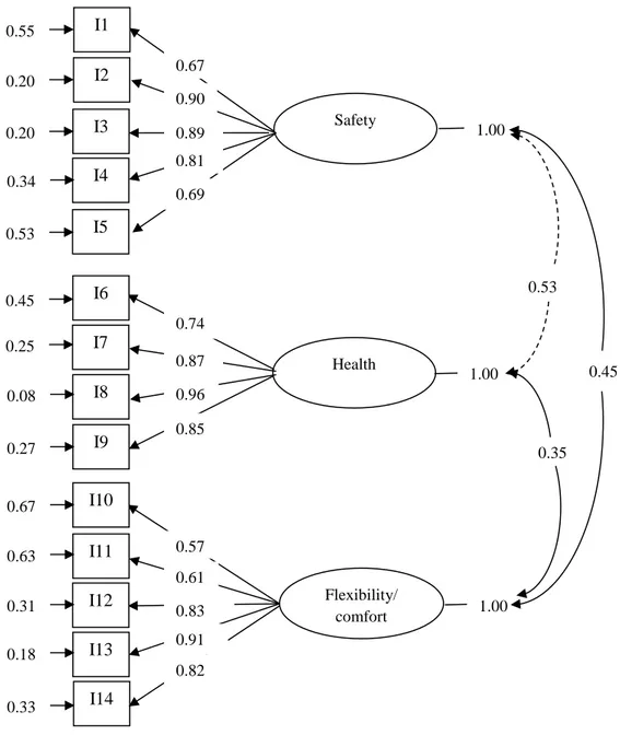
The confirmatory factor analyses were performed in LISREL 8.80 (Jöreskog & Sörbom, 1996), which is a program for structural equation modelling. As the items were measured on an ordinal scale the analyses were based on a polychoric correlation matrix and an asymptotic covariance matrix to correct the Chi-square for non-normality. We saved the factor scores for the latent variables (factors) and create a dummy variable by separating the health variable into two parts of equal size, representing high and low attitude to health and cycling. The dummy variable was used in the subsequent analyses.
The following items were included in the confirmatory factor analyses as indicator variables for each of the three latent variables.
Safety:
I1 = Separated bicycle path from footpath
I2 = Separated bicycle path from motorized traffic
I3 = The distance feels safe to bicycle regarding traffic safety I4 = Lighted bicycle paths
I5 = Good/safe bicycle parking at the destination Health:
I6 = A time-efficient way to exercise
I7 = A good way to keep weight/lose weight I8 = Improves fitness
I9 = Good for one’s own health Flexibility/Comfort:
I10 = Avoid traffic jams
I11 = Avoid congestion in public transport I12 = Is not dependent on times/departures I13 = Control over the travel time
31
In Figure 1, the result from the confirmatory factor analysis in the handed-out study is
presented. The Chi-square value is 556.15 (df = 74), p < 0,001, RMSEA = 0,072, CFI = 0,98, and SRMR = 0,079. The Chi-square value is significant which means that the estimated model do not fit the data well. However, this is more a rule than an exception, especially when the sample size is large. Therefore, there are a lot of other goodness of fit tests to use. The ones above are among the most common and shows that the fit of the estimated model is reasonable.
Figure A1. A confirmatory factor analysis of the latent variables safety, health and flexibility/comfort in the handed-out study.
Flexibility/ comfort Safety Health 1.00 1.00 1.00 0.40 0.51 0.42 0.91 0.70 0.63 I3 0.18 I4 0.30 I5 0.78 0.82 0.96 I6 0.33 I7 0.38 I8 0.57 0.80 0.56 I9 I10 I11 I2 I1 I12 I13 I14 0.87 0.74 0.91 0.83 0.85 0.60 0.28 0.52 0.08 0.17 0.68 0.69 0.36 0.24 0.45
32
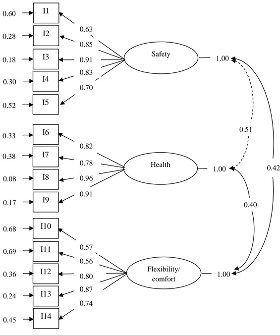
In Figure 2, the result from the confirmatory factor analysis in the mailed-out study is
presented. The Chi-square value is 304.44 (df = 74), p < 0,001, RMSEA = 0,068, CFI = 0,98, and SRMR = 0,061. The Chi-square value is significant, indicating a bad fit, but the rest of the goodness of fit tests show that the fit of the estimated model is reasonable.
Figure A2. A confirmatory factor analysis of the latent variables safety, health and flexibility/comfort in the mailed-out study.
Flexibility/ comfort Safety Health 1.00 1.00 1.00 0.35 0.53 0.45 0.89 0.69 0.67 I3 0.20 I4 0.34 I5 0.87 0.74 0.96 I6 0.45 I7 0.25 I8 0.57 0.83 0.61 I9 I10 I11 I2 I1 I12 I13 I14 0.91 0.82 0.85 0.81 0.90 0.55 0.20 0.53 0.08 0.27 0.67 0.63 0.31 0.18 0.33