A Test-Ordering Based Temperature-Cycling Acceleration Technique for 3D Stacked ICs

A Test-Ordering Based Temperature-Cycling

Acceleration Technique for 3D Stacked ICs

Nima Aghaee, Zebo Peng and Petru Eles

Linköping University Post Print

N.B.: When citing this work, cite the original article.

The original publication is available at www.springerlink.com:

Nima Aghaee, Zebo Peng and Petru Eles, A Test-Ordering Based Temperature-Cycling

Acceleration Technique for 3D Stacked ICs, 2015, Journal of electronic testing, (31), 5,

503-523.

http://dx.doi.org/10.1007/s10836-015-5541-5

Copyright: Springer Verlag (Germany)

http://www.springerlink.com/?MUD=MP

Postprint available at: Linköping University Electronic Press

http://urn.kb.se/resolve?urn=urn:nbn:se:liu:diva-123489

A Test-Ordering Based Temperature-Cycling

Acceleration Technique for 3D Stacked ICs

Nima Aghaee*_{, Zebo Peng, and Petru Eles}

Embedded Systems Laboratory (ESLAB), Department of Computer and Information Science, Linkoping University, 58183 Linkoping, Sweden

{nima.aghaee, zebo.peng, petru.eles}@liu.se +46 13 28 2231 (phone*₎

Abstract In a modern three-dimensional integrated circuit (3D IC), vertically stacked dies are

interconnected using through silicon vias. 3D ICs are subject to undesirable temperature-cycling phenomena such as through silicon via protrusion as well as void formation and growth. These cycling effects that occur during early life result in opens, resistive opens, and stress induced carrier mobility reduction. Consequently these early-life failures lead to products that fail shortly after the start of their use. Artificially-accelerated temperature cycling, before the manufacturing test, helps to detect such early-life failures that are otherwise undetectable. A test-ordering based temperature-cycling acceleration technique is introduced in this paper that integrates a temperature-temperature-cycling acceleration procedure with pre-, mid-, and post-bond tests for 3D ICs. Moreover, it reduces the need for costly temperature chamber based temperature-cycling acceleration methods. All these result in a reduction in the overall test costs. The proposed method is a test-ordering and schedule based solution that enforces the required temperature cycling effect and simultaneously performs the tests whenever appropriate. Experimental results demonstrate the efficiency of the proposed technique.

Keywords Temperature Cycling Test, Test Scheduling, Test Ordering, 3D Stacked IC

1 Introduction

Large and frequent temperature changes (i.e., temperature cycling) create fatigue and wearout in Integrated Circuits (ICs). Temperature-cycling affects ICs by causing various damages including solder joint fatigue, fracture in bond wires, and die deformation [1]. In addition to these undesirable effects, 3D stacked ICs (3D-SIC) suffer from defects related to Through Silicon Vias (TSV). TSV protrusion and void formation in TSV are two of such defects. These effects are worsened by temperature cycling [2], [3], [4]. Furthermore, some other defects including resistive opens and stress induced carrier mobility reduction can also be worsened by temperature cycling.

Temperature-cycling exacerbates a number of defect mechanisms, as pointed out above. Therefore, operating the dies under intensive temperature cycling can effectively accelerate such failures so that they can be detected by the subsequent test, before the 3D-SIC is delivered to the customers. This procedure is called temperature-cycling acceleration [5], [6]. An example for the impact of temperature cycling on 3D-SIC is the protrusion of TSVs out of the die surface. Right after TSV fabrication, there is normally no protrusion and the TSVs have about the same length as the die’s thickness. However, after a few temperature-cycles an increase in the TSV length may be observed. The TSV length will continue to increase with the number of cycles [2], [3]. After a certain amount of temperature cycling, the TSV length approaches a maximum level. Further temperature cycling will have almost no effect on the TSV length, afterwards. The TSV protrusion can be further exacerbated by the electrical current it carries [2], [3]. Therefore, operating the IC during this procedure (letting the current to flow) speeds up the cycling acceleration.

The existing procedure for temperature-cycling acceleration is based on one or multiple temperature chambers [6]. Although this procedure is usually affordable for 2D ICs, it is likely to be too expensive for 3D-SICs. Due to TSV-related defects, a larger number of dies manufactured to be a part of a 3D-SIC may require cycling acceleration compared with 2D ICs. Moreover, 3D-SIC manufacturing process includes multiple bonding stages. Corresponding to these bonding stages, pre-, mid-, or post-bond tests are introduced in order to avoid: (1) wasting a good die bonded to a bad die or stack, (2) wasting bonding effort for bonding bad dies or stacks, and (3) wasting packaging effort spent on a bad stack. Based on the cost breakdown, temperature-cycling acceleration could be beneficial at one or multiple test stages. Integrating the temperature-cycling acceleration with the tests that are performed at different stages and eliminating the need for temperature chambers will reduce the overall manufacturing costs.

Modern core-based system-on-chips, including 3D-SICs, experience excessively large test power densities [7], [8], especially since the tests are mostly scan-based. High power densities lead to excessively high temperatures, in particular for the middle dies in a 3D-SIC. Therefore, temperatures should be taken into account when planning the test process [9], [10]. This otherwise undesirable thermal effect is, however, utilized in this paper to generate large amounts of temperature-cycling. Temperature-cycling acceleration is achieved by frequent switching between high power tests that heat up the IC and pauses that allow for cooling.

A deliberate pause for cooling is called a cooling interval. It is the time interval that no stimuli are applied to a core and, therefore, the core’s temperature decreases. Some cooling intervals are usually present in the original test schedule for thermal-safety reasons. More intensive temperature-cycling acceleration can be achieved by introducing additional cooling intervals and stronger heating sequences into the process. A stronger heating sequence consists of stimuli that generate larger switching activities in a core and, therefore, increases the core’s temperature faster than usual. The mixture of cooling intervals and heating sequences can generate the required temperature-cycling acceleration effect.

A test sequence’s bit streams define the circuit-under-test’s power dissipation in combination with the previously applied test sequence (circuit’s state) as well as the core’s power-related properties. Consequently, the power dissipation generated by a series of tests depends on the order in which they are applied [11]. This phenomenon is employed in this paper in order to produce extreme power values for tests as well as heating sequences and consequently achieve a high speed temperature-cycling process.

This paper presents a schedule-based technique that integrates temperature cycling acceleration with testing procedure. The cycling acceleration is achieved by mixing heating sequences and cooling intervals with test sequences in an efficient order. Furthermore, tests and heating sequences are reordered so that a rapid testing and acceleration process is achieved. The proposed technique is in contrast with the existing approaches that are based on temperature chambers and can be impractical for 3D-SICs due to their unaffordable costs and limitations.

The rest of the paper is organized as follows. The related works are reviewed in Section 2. The preliminaries are introduced in Section 3. Section 4 presents motivational examples. Section 5 describes the problem formulation. Section 6 introduces a baseline method, the three-phase approach. Section 7 is the proposed integrated approach. Section 8 presents the experimental results and Section 9 presents the conclusion. A quick reference guide including abbreviations and notations is given in Section 10.

2 Related Works

2.1 Power Issues during Test

A large portion of modern ICs are core-based designs. Besides, the growing portion of 3D stacked ICs are also core-based. The main test techniques for all these ICs are scan based. A circuit’s switching activity depends on the changes of its bits caused by the difference between the current and the previous test as well as the state of the scan chain’s flip flops. The scan chain’s state is mainly determined by the previous tests. This phenomenon is utilized in a number of test scheduling techniques to modify the tests’ power profiles, as reviewed below.

A test power reduction technique based on test vector ordering is proposed in [11], [12]. The objective is to minimize the tests’ average switching activity. It is demonstrated that the test ordering problem is NP-hard. Consequently, a greedy approach for finding a low-power test order is proposed. An elaborate power model based on the transition count in the scan chain is also used [11], [12].

A test ordering technique for power reduction is also proposed in [13]. A close connection between the actual number of transitions and the Hamming distance between tests is confirmed. Consequently, a fast algorithm to calculate Hamming distances is used instead of the actual transition count which is hard to calculate. A greedy heuristic is then used to find a low power test order [13].

Another test ordering technique for power reduction is proposed in [14]. The circuit-under-tests’ switching activities are approximated by Hamming distances between the subsequent tests. The problem is equivalent to a travelling salesman problem. An ILP estimation and Christofides algorithm are employed to find a low-power test order [14].

A method for reducing the Test Application Time (TAT) while respecting a power budget is proposed in [15]. The method focuses on the test power peaks. These peak values depend on the order of the tests. The tests are reordered so that the power peaks for different cores are not overlapping. This leads to a minimized TAT under power constraints [15].

Reducing power variations in order to reduce the temperature variations during burn-in is discussed in [16], [17]. The variation is reduced through test reordering. An ILP approach as well as a greedy algorithm are used to properly reorder the tests. An efficient transition counting method is proposed to rapidly estimate the test power values [16], [17].

Peak power reduction by reordering the tests is studied in [18]. The peak power values are represented by a complete directed graph. Consequently a number of graph based techniques are employed to reduce the peak power. Removing those edges that their peak power is larger than a certain threshold is one of the pre-processing techniques. After that, the remaining graph is searched for a Hamiltonian path. Other techniques such as repeating a test, adding an all-zero test, and adding an all-one test are also studied [18].

2.2 Temperature Cycling and Scheduling Techniques

Existing temperature-cycling acceleration techniques are based on using one or multiple temperature chambers followed by the final test [5], [6]. This approach, in many cases, is too expensive to be performed at pre-, mid-, and post-bond stages for 3D-SICs. The shortcomings of the traditional approach include costs for running the temperature chambers as well as the time and equipment required for handling the dies/stacks between test equipment and chambers. In order to avoid these costs, in current practice, some or even all of the temperature-cycling acceleration operations are avoided. Therefore, the temperature-cycling related early-life failure rates in the final products will not be as low as it can be.

Our proposed approach for temperature cycling acceleration is mainly based on test scheduling. A number of test thermal issues that are handled using schedule-based techniques are reviewed as follows.

A burn-in technique is proposed in [19] to enforce specific temperature gradients on an IC. This results in an effective burn-in process for gradient-dependent early-life defects. A test technique is proposed in [20] to perform tests while specific temperature gradients are enforced on the IC. This helps to detect gradient-dependent defects that are usually related to signal delay and clock jitter. Temperature-gradients locations and magnitudes are represented by temperature-maps. An efficient temperature map ordering technique is proposed in [21]. The proper map order leads to faster burn-in and shorter test application time.

The usage of heating sequences is already discussed in the introduction which can be used in the temperature map enforcement approach. Heating sequences can be simply obtained by cloning of the high power tests. But, in order to have more effective heating sequences, input stimuli that generate even larger switching activities must be found. Authors in [22] have introduced an automated framework for finding high power test programs. The proposed approach is based on a meta-heuristic that generates alternative test programs and evaluates their power consumption. The alternatives with promising power consumptions are then used to generate the next generation of the test program alternatives [22]. A similar approach may be used in order to generate high power heating sequences.

A linear programming approach is used in [9] to generate thermally-safe test schedules for 3D-SICs. A temperature-based test partitioning technique is introduced in [23] in order to generate thermally-safe test schedules with a minimal test application time. A thermal-aware test scheduling approach is introduced in [10] for stacked multi-chip ICs. It minimizes the vertical temperature differences among different dies throughout the 3D IC during the test.

Two different methods for detecting temperature-dependent defects are introduced in [24] and [25]. These methods perform the tests only when the cores’ temperatures are kept within the specified range for the particular test. The focus of these papers is on the temperature of the individual cores that are under test and the temperatures of other cores are not considered.

Speeding up the test by carefully planning safety margins that counteract negative effects of process variation is addressed in [26], [27]. The test temperatures are kept sufficiently low by introducing cooling intervals into the test schedule. The cooling intervals are carefully planned using temperature simulations. In addition to a fast temperature simulation technique, an adaptive scheduling approach is proposed in [27].

These existing methods for managing the chips’ temperatures focus on keeping the temperatures under a global upper temperature limit (to prevent overheating) or to respect upper and lower bounds for cores (in order to target temperature-dependent or gradient-dependent defects). In all above cases, cores’ temperatures are considered independent of their cycling effects.

Since burn-in was mentioned above, it must be pointed out that the temperature-cycling is different from the conventional burn-in. These two aim at accelerating different aging mechanisms. Cycling acceleration will not accelerate aging mechanisms identical to those that burn-in does and vice versa. To briefly explain this difference, let us focus only on two aging mechanisms. During burn-in the device is operated in a very hot environment with increased voltage to accelerate electromigration. This must continue for a relatively long time to allow for sufficient migration (detectable atomic built-up or depletion). On the contrary, simply operating the device at a single temperature does not create cycling-related material fatigue. It is the variation of the mechanical stress (as a result of varying temperature) that does it. The required amounts of burn-in and cycling are decided based on analytical, experimental, and empirical studies that are outside the scope of this paper. In this paper we solely focus on temperature-cycling and assume that the required amount of cycling is given by user.

The first proposal to integrate temperature cycling acceleration with test procedure was made by us in [28]. The current paper has built on the preliminary results introduced in [28] and develops an efficient technique to order the tests and heating sequences to achieve a high speed temperature cycling process. Furthermore, an accurate cycling related acceleration model that, also, includes Arrhenius acceleration is used in this paper. Additionally, this paper offers a technique to efficiently mix the remaining normal tests1 _{with cycling tests}1_{. The proposed technique provides controlled}

temperature-cycling acceleration without utilizing temperature chambers.

3 Preliminaries

3.1 Circuit under Test and Test Access Mechanism

It is assumed that there are 𝑀 modules (cores) in the 3D-SIC under test. These modules are located on different levels of stacked dies. The modules that are on different layers are connected using TSVs. Tests for each module can be started and stopped independent of other modules. The modules could be cores with core wrappers in a core-based design. The extension of this scenario to 3D-SIC is proposed as the IEEE P1838 standard [29]. Test stimuli are, therefore, transferred through a Test Access Mechanism (TAM) to the relevant module. It is assumed that the TAM only affords 𝑊 (a positive integer number) modules to be tested at the same time. Other modules, therefore, have to queue up and wait for TAM access.

3.2 Thermal Model

In order to obtain the temperature values from power values, a thermal model that describes the thermal behavior of the IC must be used. The model used in this paper is HotSpot [30] and its extension for 3D ICs [31]:

𝑨 ×_𝑑𝑡𝑑𝜣 + 𝑩 × 𝜣 = 𝑷 (1)

All the characteristics of the thermal model are captured in two matrices 𝑨 and 𝑩. 𝜣 is the temperature vector and 𝑷 is the power. 𝜣 and 𝑷 consist of 𝜃𝑚s and 𝑃𝑚s, respectively, put together

in a vector format. Index 𝑚 indicates the relevant module. There are a total of 𝑀 modules (𝑚 = 0, 1, … , 𝑀 − 1). Equation 1 can be solved for time-domain assuming that the power values are constant during a period of time equal to 𝜏, as follows [27]:

𝜽𝜏 _{= 𝜶 × 𝜽}0_{+ 𝜷 × 𝑷 (2)}

The initial temperature is expressed by 𝜽0 _{and the temperature after a period of 𝜏 seconds (note that}

a fraction of a second is used in practice) is represented by 𝜽𝜏. Matrices 𝜶 and 𝜷 are obtained as follows [27]:

𝜶 = exp(−𝑨−1_{× 𝑩 × 𝜏) (3a)}

and

𝜷 = (𝑰 − 𝜶) × 𝑩−1 _(3b)

The identity matrix is denoted by 𝑰. The above equations are explained in the following case study, assuming that there is only one module (𝑀 = 1) with its heat capacitance denoted by 𝐶 (analogous to 𝑨). The heat resistance between the module and the ambient is equal to 𝑅 (analogous to 𝑩−1_{). In}

this case, Equation 2 can be re-written as: 𝜃𝜏_{= 𝜃}0_{∙ exp (−} 𝜏

𝑅∙𝐶) + 𝑃 ∙ 𝑅 ∙ (1 − exp (− 𝜏

𝑅∙𝐶)) (4)

Since there is only one module, the vectors and matrices are reduced to scalar values. A larger initial temperature (𝜃0_{), power (𝑃), or resistance (𝑅) results in higher final temperature (𝜃}𝜏_{), if other factors}

are kept unchanged. A larger period (𝜏) means that the contribution of the initial temperature is smaller while the effect of power on the final temperature is larger. In the vector form, increasing the period translates into a decreased 𝜶 and an increased 𝜷. A large time-constant (𝑅 ∙ 𝐶) means that the initial temperature takes longer to lose its effect while power takes longer to noticeably affect the final temperature. In the vector form, increasing the time-constant translates into an increased 𝜶 and a decreased 𝜷.

3.3 Temperature Cycling Model

The effect of temperature cycling can be described based on the Amount of Temperature Cycling induced fatigue (denoted by ATC𝑚 for module 𝑚). Based on the Arrhenius-Coffin-Manson model

[1], [32], ATC is estimated as: 𝐴𝑇𝐶𝑚≅ 𝒩_𝑘𝑚 0 × ( ∆𝜃𝑚− 𝜃𝜖 𝑘1 ) 𝛾 × exp (𝜃̅̅̅̅𝑚 𝑘2) (5)

Considering module 𝑚, in this equation 𝒩_𝑚 is the number of temperature cycles and ∆𝜃_𝑚 is the amplitude of temperature changes during cycling. In the above equation, a regular cycling pattern is assumed. It means that the temperature monotonically increases from an arbitrary temperature 𝜃_𝑚𝑎 to 𝜃𝑚𝑎+ ∆𝜃𝑚 and then monotonically decreases back to 𝜃𝑚𝑎. Usually, when the actual temperature

curve is only a bit different from a regular pattern, the average amplitude is used for ∆𝜃_𝑚. ∆𝜃_𝑚 must be larger than 𝜃𝜖 _{(a very small threshold value) in order to be considered in the temperature cycling}

calculations. However, it is not unusual to completely ignore 𝜃𝜖 since the typical temperature changes are much larger than 𝜃𝜖_{. The effect of the average temperature is captured in the exponential}

term. The average temperature is expressed by 𝜃̅̅̅̅. 𝜃_𝑚 𝜖, 𝑘₀, 𝑘₁, 𝑘₂, and 𝛾 are constants that are obtained analytically or empirically by reliability analysts. A comprehensive explanation and details of Equation 5 can be found in [1] and [32]. As Equation 5 suggests, a large number of cycles, 𝒩𝑚,

a large temperature swing, ∆𝜃𝑚, or a large average temperature, 𝜃̅̅̅̅, will result in a large cycling 𝑚

effect.

4 Motivational Examples

4.1 ATC Rate for a Simple Scenario

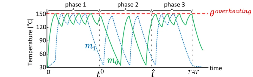
As an example, consider an IC with two modules (𝑀 = 2). Assume that the TAM can only support one module to be tested at a time (𝑊=1). Assume that 𝜃𝑜𝑣𝑒𝑟ℎ𝑒𝑎𝑡𝑖𝑛𝑔_{= 150℃ and 𝜃}𝑎𝑚𝑏𝑖𝑒𝑛𝑡_{= 30℃.}

The required amounts of temperature cycling are 𝐴𝑇𝐶0𝑅 and 𝐴𝑇𝐶1𝑅 for modules 𝑚0 and 𝑚1,

respectively. In this paper, tests that target cycling-dependent defects are called cycling tests and the other tests are called normal tests. Cycling tests can only be applied after the required amount of temperature cycling, 𝐴𝑇𝐶𝑚𝑅, is achieved.

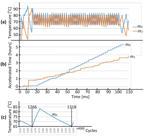
A three-phase approach is introduced here: In phase 1, normal tests are scheduled. A thermal aware scheduling of tests based on the proposed approach in [33] is used. The corresponding temperature curves are shown in Fig. 1 (green for 𝑚0 and blue for 𝑚1). The normal tests for module 𝑚 end at

𝑡𝑚0. Phase 1 starts at time 0 and end at 𝑡0 that is defined as max 𝑚 {𝑡𝑚

0_}.

Phase 2 starts by evaluating the ATC generated in phase 1. This value is less than the required 𝐴𝑇𝐶𝑚𝑅

in this example. Therefore, phase 2 will generate additional temperature cycling. This is done by applying the heating sequences and cooling intervals. Corresponding temperature cycles can be seen in Fig. 1 from 𝑡0 _{to 𝑡̂. Time-point 𝑡̂}

𝑚 marks the point when the required 𝐴𝑇𝐶𝑚𝑅 is achieved for module

𝑚. Phase 2 ends when all required ATCs for all modules are met. This point is marked with 𝑡̂ that is defined as max

𝑚 {𝑡̂𝑚}. After this, phase 3 starts by applying the cycling tests. Phase 3 ends when

Always, a small TAT is desirable. Test application time from 0 to 𝑡0 _{and from 𝑡̂ to 𝑇𝐴𝑇 is already}

minimized by the given third-party test scheduling algorithm. The only TAT reduction opportunity in this three-phase approach is to speed up phase 2. This means that a large ATC should be achieved in a short time. Therefore, 𝐴𝑇𝐶𝑚(𝑡)/𝑡 should be maximized. Here we assume a uniform periodic

temperature profile that means all cycles have the same amplitude. Moreover, for this motivational example we assume that in Equation 5: 𝑘0= 1, 𝑘1= 1, 𝑘2≫ 𝜃̅̅̅̅, and 𝜃𝑚 𝜖 ≪ ∆𝜃𝑚.

Since it is assumed that 𝑘2≫ 𝜃̅̅̅̅, the exponential term can be ignored for the moment. Furthermore, 𝑚

since it is assumed that 𝜃𝜖≪ ∆𝜃_𝑚, 𝜃𝜖 could also be ignored. The ATC rate (denoted by 𝜌_𝑚 for module 𝑚) can, therefore, be defined as:

𝜌𝑚=

𝐴𝑇𝐶𝑚(𝑡)

𝑡 = 𝒩𝑚(𝑡)

𝑡 × (∆𝜃𝑚)𝛾 (6)

Frequency of temperature changes (i. e., the number of cycles per time unit) depends on the physical properties of the system and the amplitude of temperature changes, ∆𝜃𝑚. It is possible to achieve a

high frequency (i.e., a large 𝒩𝑚(𝑡)

𝑡 ) if ∆𝜃𝑚 is small. A large amplitude on the other hand, may increase

the ATC, only if it dominates the resulted reduction in the frequency.

4.2 Optimal Cycling in a Simplified Scenario

In order to clarify the tradeoff between the frequency and the amplitude of the temperature cycling, the physical properties of the system should be captured in the ATC rate equation (Equation 6). In the following this is done for a simple IC with only one module. The thermal model for such a case was discussed in Section 3.2, Equation 4. Remember that 𝐶 is the heat capacitance and 𝑅 is the thermal resistance between the module and the ambient. Assume that the heating sequence generates a power equal to 𝑃 and the power during a cooling interval is zero. Assume that the temperature varies between 𝜇 − 𝜎 and 𝜇 + 𝜎. Both 𝜇 and 𝜎 are positive real numbers.

The period of a temperature cycle is denoted by 𝑇. This period consists of a rise time denoted by 𝑇𝑟

plus a fall time denoted by 𝑇𝑓. 𝑇𝑟 is the time the temperature takes to increase from 𝜇 − 𝜎 to 𝜇 + 𝜎.

𝑇𝑓 is the time taken to decrease from 𝜇 + 𝜎 to 𝜇 − 𝜎. These values are calculated as follows. First,

the system’s differential equation is solved in the time domain similar to Equation 4 for a period of 𝑡 (i.e., 𝜏 = 𝑡):

𝜃𝑡_{= 𝜃}0_{∙ exp (−} 𝑡

𝑅∙𝐶) + 𝑃 ∙ 𝑅 ∙ (1 − exp (− 𝑡

𝑅∙𝐶)) (7)

Let us denote 𝑅 ∙ 𝐶 by 𝑅𝐶 and 𝑃 ∙ 𝑅 by 𝑃𝑅. For heating: (𝜇 + 𝜎) = (𝜇 − 𝜎) exp (−𝑇𝑟 𝑅𝐶) + 𝑃𝑅 (1 − exp (− 𝑇_𝑟 𝑅𝐶)). (8) Then 𝑇𝑟= 𝑅𝐶 × ln (𝜇−𝜎−𝑃𝑅_{𝜇+𝜎−𝑃𝑅}). (9a)

Similarly for cooling, 𝑇𝑓 can be calculated:

𝑇𝑓 = 𝑅𝐶 × ln (𝜇+𝜎_𝜇−𝜎). (9b)

The period, 𝑇, is calculated as follows:

𝑇 = 𝑇𝑟+ 𝑇𝑓= 𝑅𝐶 × ln ((𝜇−𝜎−𝑃𝑅)(𝜇+𝜎)_{(𝜇+𝜎−𝑃𝑅)(𝜇−𝜎)}). (10) Now, the ATC rate (Equation 6) could be re-written incorporating the physical properties of the system:

Fig. 1 Temperature curves for the three-phase approach. Curves are illustrative. 90 60 0 Te m p er at u re [ o C ] 150 30 time 120 phase 3 phase 2 phase 1

𝜌𝑚= (2𝜎) 𝛾

𝑅𝐶×ln((𝜇−𝜎−𝑃𝑅)(𝜇+𝜎)_{(𝜇+𝜎−𝑃𝑅)(𝜇−𝜎)})= (2𝜎)𝛾

𝑅𝐶×ln(𝜉). (11)

Let us first focus on the optimal value for 𝜇, assuming that 𝜎 is constant. In this case optimality happens when the denominator in Equation 7 is minimized. Considering a realistic situation, this is equivalent to finding the minimum for

𝜉 =(𝜇−𝜎−𝑃𝑅)(𝜇+𝜎)_{(𝜇+𝜎−𝑃𝑅)(𝜇−𝜎)}. (12)

Following a closed-form approach:

𝑑

𝑑𝜇𝜉 = 0 →

(2𝜇−𝑃𝑅)((𝜇+𝜎−𝑃𝑅)(𝜇−𝜎)−(𝜇−𝜎−𝑃𝑅)(𝜇+𝜎))

((𝜇+𝜎−𝑃𝑅)(𝜇−𝜎))2 = 0 (13)

The valid solution is 𝜇 = 𝑃𝑅/2. Here for the sake of simplicity, the ambient temperature was not included in the equations. Since the temperature model is a Linear Time-Invariant (LTI) system [27], the ambient temperature can be added later on. Assume that power and resistance values are so that 𝑃𝑅 = 120℃. This means that considering the ambient temperature (30℃), the IC’s temperature will increase to 150℃ if no control is applied. Thus, the optimal value for 𝜇 is 𝜇𝑂𝑝𝑡𝑖𝑚𝑎𝑙=120℃₂ +

30℃ = 90℃.

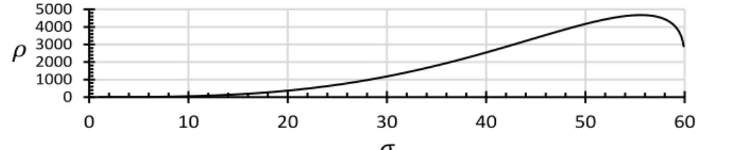
The resulted equations for finding the optimal value for 𝜎 do not have a simple closed form. Therefore, a numerical method is employed. The ATC rate 𝜌 versus 𝜎 for 𝜇 = 90℃ is plotted in Fig. 2. If 𝛾 = 4 and 𝑅𝐶 = 50 μs, then the ATC rate is maximal at 𝜎𝑂𝑝𝑡𝑖𝑚𝑎𝑙 = 55.6℃. For values of

𝜎 less than 𝜎𝑂𝑝𝑡𝑖𝑚𝑎𝑙 the ATC rate increases by increase in 𝜎. This is due to the increase in amplitude,

(∆𝜃𝑚)𝛾, dominating the decrease in frequency, 𝒩𝑚(𝑡)/𝑡, in Equation 6. For larger 𝜎 values the

ATC rate decreases by increase in 𝜎. This is due to the increase in amplitude, (∆𝜃𝑚)𝛾, being

dominated by the decrease in frequency, 𝒩𝑚(𝑡)/𝑡. In other words, a very large temperature cycle

takes too much time to complete.

If the assumption that 𝑘2≫ 𝜃̅̅̅̅ does not hold, the temperature cycling rate equation, Equation 11, 𝑚

will be as follows: 𝜌𝑚= (2𝜎) 𝛾 𝑅𝐶×ln((𝜇−𝜎−𝑃𝑅)(𝜇+𝜎)_{(𝜇+𝜎−𝑃𝑅)(𝜇−𝜎)})× 𝑒 𝜇 𝐾⁄ _{2 =} (2𝜎)𝛾 𝑅𝐶×ln(𝜉)× 𝑒 𝜇 𝐾⁄ _2. (14) The inclusion of the exponential (Arrhenius) term results in a larger (or equal) optimal 𝜇𝑂𝑝𝑡𝑖𝑚𝑎𝑙

value. Since both the exponential term and Equation 11 are increasing when 𝜇 is smaller than 𝑃𝑅/2, the optimal value cannot happen for a 𝜇 smaller than 𝑃𝑅/2. After this point, the value of Equation 11 decreases while the exponential term is increasing. The optimal 𝜇 can be in this region (𝜇 ≥ 𝑃𝑅/2). Besides, the introduction of the exponential term leads to dependency of the optimal 𝜇 on the value of 𝜎.

In the general case (without assumptions made for the motivational examples), the optimal value for 𝜇 could be very different compared with the 𝜇𝑂𝑝𝑡𝑖𝑚𝑎𝑙 obtained here. Moreover, the assumptions

made for obtaining Equation 6 will not be valid and therefore the situation will be more complicated than discussed in the above paragraph. In such situations a numerical approach is best suited to find the optimal values for 𝜇 and 𝜎. Moreover, in the general case, there are multiple modules competing for access to TAM and their interference makes the problem even more complicated, so complex that a heuristic is the only practical solution to deal with the problem.

4.3 Effect of the Test Application Order

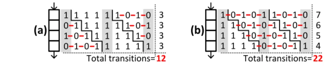
In general, the circuit under test’s consumed power depends on the order in which the tests are performed. Let us consider the scan chain itself. Different orders of the tests will result in different transition counts and thus different power values. Consider a 4-bit scan chain as shown in Fig. 3.

Fig. 2 ATC rate, 𝜌, versus 𝜎 for three-phase approach.

0 1000 2000 3000 4000 5000 0 10 20 30 40 50 60

Assume that 0101, 1111, and 1010 are the test stimuli. The order 1010-1111-0101, as shown in Fig. 3a, results in 12 transitions in the scan chain during shift-in. Another test order, 1111-1010-0101, as shown in Fig. 3b, results in 22 transitions and thus higher power dissipation. Assuming that the temperature of the core should be reduced, arranging the tests in their low power order may avoid an additional cooling interval. Alternatively, if the core is in its heating interval of the cycling process, the high power arrangement may replace an unnecessary heating sequence application. This will ensure that TAM is not unnecessarily occupied by dummy heating sequences. Both situations help to shorten the test application time.

5 Problem Formulation

As discussed before, along with pre-, mid-, or, post-bond tests, temperature-cycling acceleration might be beneficial. In this case, there will be tests that target cycling-dependent defects (i.e. cycling tests) in addition to other tests (i.e., normal tests). Normal tests are scheduled along with heating and cooling intervals in order to generate the required amount of temperature cycling. The cycling tests can be performed afterward.

The amount of temperature cycling can be easily calculated using Equation 5 if the temperature swings in a uniform periodic manner similar to Fig. 4a. In Fig. 4a five cycles with amplitudes equal to ∆𝜃 can be identified. In the general case, for example when the IC is under test, the temperature fluctuations are irregular, as shown in Fig. 4b. In this case, identifying cycles and their amplitudes is not straightforward. For such irregular patterns, the number and amplitudes of the cycles are calculated using the widely used Rainflow-counting algorithm [34].

As mentioned previously, the required amount of temperature cycling is denoted by 𝐴𝑇𝐶_𝑚𝑅. The current amount of temperature cycling generated by normal tests or heating sequences (e.g., phase 1 and phase 2 in Fig. 1), up to a given time, 𝑡, is denoted by 𝐴𝑇𝐶𝑚(𝑡). For a certain test schedule,

the temperature curves are obtained using temperature simulations. Then a fast version of Rainflow-counting algorithm, introduced in [35], calculates 𝐴𝑇𝐶𝑚(𝑡). Assuming that for 𝑡 < 𝑡̂𝑚, 𝐴𝑇𝐶𝑚(𝑡) <

𝐴𝑇𝐶𝑚𝑅, only normal tests can be performed before time 𝑡̂𝑚. The cycling tests can only be performed

after the required amount of cycling (𝐴𝑇𝐶𝑚𝑅) has been applied. Therefore, after time 𝑡̂𝑚, cycling tests

can be performed too. The test application time, 𝑇𝐴𝑇_𝑚, marks the point that testing module 𝑚 is complete. 𝑇𝐴𝑇𝑚 consists of the time spent before and after time 𝑡̂𝑚. The goal is to generate a

schedule with a minimal overall TAT. The overall test application time is defined as max

𝑚 {𝑇𝐴𝑇𝑚}.

As previously discussed, the power dissipation during a test depends on the previous test, among other factors. Assuming that test 𝑠𝑚,𝑠 for module 𝑚 immediately follows test 𝑠𝑚,𝑢, the dynamic

power is expressed by 𝑝𝑚,𝑢−𝑠𝑑 . The overall power dissipation (in the circuit under test), denoted by

𝑝𝑚,𝑢−𝑠, consists of the dynamic power, 𝑝𝑚,𝑢−𝑠𝑑 , plus the stray power, denoted by 𝑝̂ (𝑝𝑚 𝑚,𝑢−𝑠=

𝑝𝑚,𝑢−𝑠𝑑 + 𝑝̂ ). The dynamic power is caused by the circuit under tests’ switching activities. The 𝑚

stray power is defined, in this paper, as the sum of all power values that their dissipations cannot be independently controlled with existing test controls. This includes the leakage power as well as the clock networks’ power. Stray power’s exact value depends on the module’s current temperature since the leakage power depends on the temperature. In this paper, the stray power (including temperature dependent leakage) is taken into account.

Fig. 4 Temperature patterns: (a) Uniform periodic. (b) Irregular

(a) (b)

1 2 3 4 5

Fig. 3 Test orders: (a) A low power order. (b) A high power order.

(a)

(b)

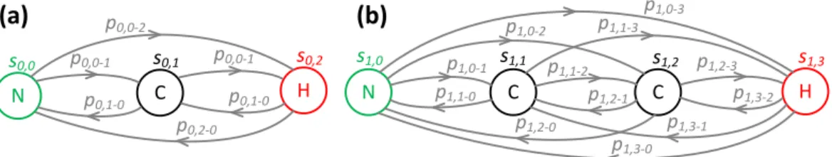
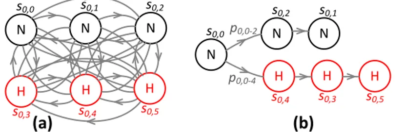
It is assumed that module 𝑚 has 𝑁_𝑚 tests including both normal and cycling tests. Relevant test properties can be captured in a test graph. Consider an IC that consists of two modules (𝑀 = 2). Assume that module 𝑚0 has two tests (𝑁0= 2) as shown in Fig. 5a. Module 𝑚1 has three tests

(𝑁1= 3) as shown in Fig. 5b. Assume that one of the tests for module 𝑚0 is a normal test (the node

is marked with N) and the other is a cycling test (marked with C). A node that corresponds to a heating sequence (marked with H) is also included in the test graph. Tests and the heating sequence for module 𝑚1 are marked in a similar manner. Total test powers are shown on the edges in Fig. 5.

Usually, in the general case, there are a number of normal and cycling tests in addition to a number of heating sequences.

At each time point, during the test, there could be some tests that cannot be performed. This is due to a number of reasons including the limited capacity of the TAM as well as the cycling tests that cannot be performed before the required ATC is applied. A validity checker is used to make sure that the scheduling algorithm takes these limitations into account. The validity checker updates the set of Valid Tests (VaT) if a new test can be performed in parallel with the tests that are already selected for the current time point. It also makes sure that any test that cannot be applied in parallel with the currently selected tests does not remain in VaT. This is based on the knowledge of previously applied tests as well as the partial set of tests selected to be applied next. Moreover, the current amount of the ATC is also taken into account. For example, assume that in Fig. 5 normal tests (𝑠0,0 and 𝑠1,0) have been performed previously. Assume that 𝑠0,1 is already selected to be

applied next and the required ATC for 𝑚1 is already achieved. In this case VaT is {𝑠1,1 𝑠1,2 𝑠1,3}.

Meaning that 𝑠1,1, 𝑠1,2, or 𝑠1,3 can be applied in parallel with 𝑠0,1 without violating TAM limit or

ATC requirement. Although using 𝑠1,3 (i.e., the heating sequence) does not make sense since the

required ATC is already achieved, it would be a valid choice from the VaT’s point of view. Note that the heating sequences can be applied repeatedly, as needed, while repeating the tests is usually unnecessary.

The goal is to schedule the tests so that all the cycling tests are performed after the required amount of ATC is achieved and the overall test application time (including the cycling process) is minimized. This is achieved by scheduling and reordering the tests and the heating sequences. High power test stimuli and heating sequences can increase the modules’ temperatures. A module may become so hot that unrealistic failures show up and even the device gets damaged. In order to avoid these undesirable overheating situations, the modules’ temperatures must be kept below the overheating temperature (𝜃𝑜𝑣𝑒𝑟ℎ𝑒𝑎𝑡𝑖𝑛𝑔_{) at any time. The overheating temperature is equal to the}

temperature limit minus a safety margin to ensure thermal safety. The power dissipation during a pause is equal to the stray power, 𝑝̂ (including leakage). 𝑚

The problem can be described as follows. The inputs to the suggested technique include the IC’s thermal model, the IC’s electrical model (e.g., specification of the TAM and power-related specifications), the test graph (i.e., the cycling tests, normal tests, and the switching activities of the tests and heating sequences), the ambient temperature (𝜃𝑎𝑚𝑏𝑖𝑒𝑛𝑡_{), and the required amount of}

temperature cycling, 𝐴𝑇𝐶𝑚𝑅. The objective is to minimize the test application time. The output is the

corresponding schedule that guides the application of the tests and heating sequences in proper order so that all the tests are performed rapidly and correctly.

The generated schedule will imply, for each of the modules, a certain ordering of the test graph’s node. The ordering can be represented by a directed path in each of the original test graphs (e.g., graphs in Fig. 5). This directed path must visit each test node at least once and may visit heating nodes as many times as needed. Applying a test or a heating sequence is equivalent to visiting the corresponding test or the heating node. The test ordering and scheduling can also be viewed as converting the original test graph into a final path-graph. A path-graph is defined as a graph with only one directed path that connects all the nodes. There is no other edge in a path-graph except those on this unique path. The final path-graph must include all of the test nodes, while the heating

Fig. 5 Test graphs for (a) module 𝑚0 (b) module 𝑚1. Test graphs consist of normal (N), cycling

(C), and heating (H) nodes.

(a)

(b)

nodes are included as needed. The ordering algorithm decides at which point to insert a node taken from the original test graph into the final path-graph.

6 Three-Phase Approach

The basics of the three-phase approach are briefly explained in Section 4.1. Section 4.2 presents a technique to find the best temperature interval (𝜇 − 𝜎 to 𝜇 + 𝜎) for a simplified scenario. As discussed before, if the coefficient 𝑘2 (in Equation 5) is much larger than the average temperature

(𝑘2≫ 𝜃̅̅̅̅) and the high temperature level (𝜇 + 𝜎) is smaller than the overheating temperature, 𝑚

𝜃𝑜𝑣𝑒𝑟ℎ𝑒𝑎𝑡𝑖𝑛𝑔_{, everything in Section 4 would be fine. However, often these assumptions are not valid,}

for example the overheating temperature may be relatively low compared with 𝜇 + 𝜎. For the example in Section 4.2, 𝜇 + 𝜎 is equal to 145.6℃ while the overheating temperature might be 120℃. There are some other complications, as well. In practice there are a number of modules, instead of one, and their temperatures depend on each other due to heat transfer. Furthermore, the power values fluctuate with time. Besides, power values include the stray powers that depend on the temperature due to the temperature dependent leakage currents. Additionally, the modules may not be able to receive their heating sequences at desired times due to the TAM limitation. New approaches capable of taking all these situations into account are, therefore, proposed in the following.

As discussed in Section 4.1, in phase 1 and 3 the tests are scheduled using a thermally safe third-party algorithm. It is assumed that these algorithms perform optimization to reduce the test application time. Our focus will therefore be on phase 2 where new algorithms can be designed to minimize the test application time. This was demonstrated using a small example in Section 4.2. Assume that in phase 2 the temperature of module 𝑚 is intended to swing between a low temperature level 𝜃𝑚𝐿 and a high temperature level 𝜃𝑚𝐻 (𝜃𝑚𝐿 < 𝜃𝑚𝐻). In comparison with the example in Section

4.2, 𝜃𝑚𝐿 and 𝜃𝑚𝐻 have roles similar to that of 𝜇 − 𝜎 and 𝜇 + 𝜎, respectively.

The heating sequences are assumed to be powerful enough to raise the module’s temperature to 𝜃𝑚𝐻.

The high temperature level should always be lower than the overheating temperature (𝜃𝑚𝐻<

𝜃𝑜𝑣𝑒𝑟ℎ𝑒𝑎𝑡𝑖𝑛𝑔_{) to avoid any kind of damage. Since all the normal tests and all the cycling tests are to}

be separately scheduled using third party algorithms and then performed in two isolated phases (phase 1 and 3), there is no need to represent them in the test graph. Consequently the test graph reduces to only include the heating nodes (nodes marked with H in Fig. 5). This simplifies the problem of finding a proper path in this reduced graph. A greedy approach is used here and the heating node that offers the highest heating power is selected to follow the current node.

Immediately after the temperature reaching its peak at 𝜃𝑚𝐻, a cooling interval is introduced to reduce

the temperature back to 𝜃𝑚𝐿. Then, for the sake of a fast cycling, the heating sequence must be

immediately applied again. However, the TAM might not be available at this moment. Consequently, the temperature may fall below 𝜃𝑚𝐿 from time to time. An on-the-fly approach is used

to schedule the heating sequences for phase 2 based on the simulated temperatures. The temperatures that are obtained by simulation are then compared with 𝜃𝑚𝐿 and 𝜃𝑚𝐻 in order to generate the schedule.

Heating sequences for different modules will compete for access to TAM. The priority is decided based on the following equation.

𝜋𝑚= (𝜃𝑚𝐿 − 𝜃𝑚) × 𝐴𝑇𝐶𝑚 𝑅

𝜖+𝐴𝑇𝐶_𝑚 (15)

The priority is higher if the module’s current temperature is much below 𝜃𝑚𝐿. Note that the priorities

are calculated only for modules that need heating, therefore 𝜃𝑚< 𝜃𝑚𝐿. The reason for the inclusion

of this difference term (i.e., 𝜃𝑚𝐿 − 𝜃𝑚) in the priority assessment is that if a module gets really cold,

it takes too much time to warm it up again. Therefore, it is a good idea to give a higher priority to the colder modules. A module that has a large amount of temperature cycling left to fill has also a higher priority. This is indicated by 𝐴𝑇𝐶𝑚

𝑅

𝜖+𝐴𝑇𝐶_𝑚. Such a module is likely to need a relatively long time

to achieve its required ATC. Consequently, it is likely that at the later stages of phase 2 this module remains alone. This implies that the interleaving opportunities for TAM access will be reduced. Consequently TAM utilization may decrease and test application time may increase. A small value, 𝜖, is added to the denominator in order to prevent numerical problems when ATC is zero (e.g., at the beginning of phase 2, if there have not been any normal test). Both 𝜃𝑚 and 𝐴𝑇𝐶𝑚 depend on

The test application time for the schedules generated by this on-the-fly approach depends on 𝜃𝑚𝐿 and

𝜃𝑚𝐻. These temperature levels could assume a range of values provided that 𝜃𝑚𝑠𝑡𝑟𝑎𝑦≤ 𝜃𝑚𝐿 < 𝜃𝑚𝐻<

𝜃𝑜𝑣𝑒𝑟ℎ𝑒𝑎𝑡𝑖𝑛𝑔_{. The temperature that corresponds to the stray power is called stray temperature and is}

denoted by 𝜃𝑚𝑠𝑡𝑟𝑎𝑦 (always 𝜃𝑎𝑚𝑏𝑖𝑒𝑛𝑡≤ 𝜃𝑚𝑠𝑡𝑟𝑎𝑦< 𝜃𝑜𝑣𝑒𝑟ℎ𝑒𝑎𝑡𝑖𝑛𝑔). Temperature of a module cannot be

lower than this because of the stray power dissipation (including leakage). The combination of these temperature levels (𝜃𝑚𝐿 and 𝜃𝑚𝐻) among different modules affects the test application time. The

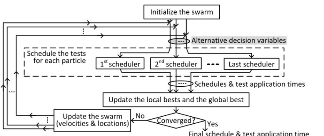
proper values for these decision variables will be found in an external optimization loop, as shown in Fig. 6. In the inner scheduling loop, the temperature levels (i.e., decision variables) defined by the outer optimization loop are used to generate the schedule. In Fig. 6, the scheduler boxes inside the dashed box represent multiple copies of the inner scheduling algorithm. However only one of such schedulers is sufficient to perform the optimization, multiple of them are used in parallel to speed up the procedure.

The outer optimization loop makes use of a Particle Swarm Optimization (PSO) algorithm. PSO is a well-known iterative population-based optimization metaheuristic. For each alternative solution in the PSO’s population, on-the-fly scheduling is performed (inside the dashed box in Fig. 6) to compute the cost function (i.e., TAT). A canonical form of PSO [36] is used in this paper in a straightforward manner. The algorithm starts from a random initial population, similar to other population based metaheuristics (e.g., evolutionary methods). The population is referred to as a

swarm in PSO terms. An individual in the population is referred to as a particle. Each particle goes

through a number of alternative solutions, one at a time, as the algorithm iterates. Each particle has a location in the search space (i.e., the current alternative solution). A particle records the best solution it has ever encountered, the local best. The swarm records the best solution its particles have ever encountered, the global best. Based on these best solutions and the previous alternative solution a velocity is determined which also incorporates some randomization [36]. Velocity is the vector that determines the next location for a particle. The particles move throughout the search space in a guided random manner until they converge to a near optimal solution.

7 Integrated Approach

Let us assume, now, that the orders in which normal test nodes (e.g., nodes marked with N in Fig. 5) must be visited are given. Furthermore, assume that the order for heating sequence nodes (e.g., nodes marked with H in Fig. 5) are also given. This means that the original test graph is broken down into a number of sub-graphs. This includes two separate directed path-graphs, one for normal tests and the other for the heating sequences among other sub-graphs. This simplified scenario which involves two separate path-graphs will be discussed first and a path-graph scheduling algorithm will be introduced in Sections 7.1–3. Afterwards, Section 7.4 explains how to employ this path-graph scheduling algorithm to solve the original problem that involves the original test graph (i.e., the problem formulation in Section 5). Fig. 7 shows how these components are put together. An example in the following paragraphs (using Fig. 8) explains some of the blocks of Fig. 7. The remaining blocks are explained later on.

Fig. 6 Particle swarm optimization algorithm used to minimize the test application time. Inside the

dashed box, copies of the scheduling heuristics are performed in parallel for a number of particles.

Schedule the tests

for each particle ₁st _{scheduler 2}nd _{scheduler Last scheduler}

Converged?

Update the local bests and the global best Update the swarm

(velocities & locations)

Alternative decision variables

Schedules & test application times

No

Yes

Final schedule & test application time Initialize the swarm

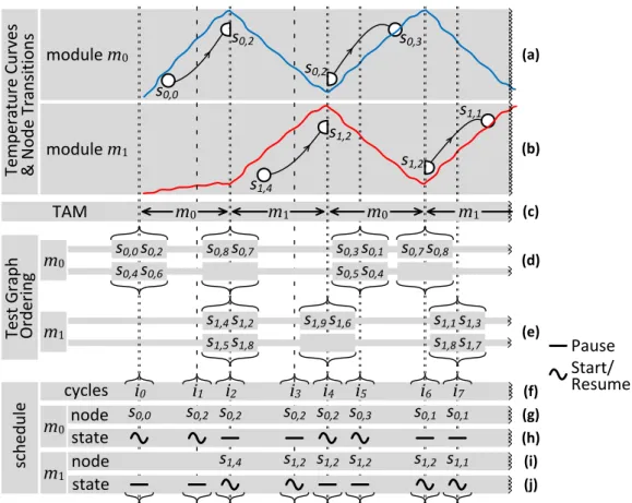
A small example, in Fig. 8, explains how all these blocks work together to generate a schedule1_{. Let}

us assume that path-graph scheduling (i.e., Path-graph scheduling block in Fig. 7) determines that the module 𝑚0 must receive heating at 𝑖0 test cycle. Test cycles are shown in Fig. 8f. It asks test

graph node ordering (i.e., Node ordering block in Fig. 7) for options. Test graph ordering replies by two options (as shown in Fig. 8d): The first option is [𝑠0,0, 𝑠0,2] that is a path-graph consisting of

high power normal test nodes. The second option is [𝑠0,4, 𝑠0,6] that consists of heating nodes. This

interaction is depicted in Fig. 7 as the loop between path-graph scheduling block and node ordering block. The output of the node ordering block is monitored to determine if all tests are completed. The path-graph scheduling decides to go on with [𝑠0,0, 𝑠0,2]. Now, the power values are known and

temperatures simulation is performed to obtain the temperatures. This interaction is depicted in Fig. 7 as the loop between path-graph scheduling block and temperature simulator block. The simulated temperatures are plotted in Fig. 8ab. As module 𝑚0 heats up, module 𝑚1 is slightly warmed up by

the transferred heat from 𝑚0. It is assumed that the die in this example consists of only two modules.

Moreover, it is assumed that the test access mechanism provides access to only one of the modules at a time. The module that occupies the TAM is depicted in Fig. 8c.

Every decision (i.e., change in the schedule) is recorded in the schedule as a new entry. Each entry consists of the corresponding cycle in addition to the node and state for each and every module. For example a decision was made at cycle 𝑖0 to start 𝑠0,0. This is registered in the schedule as shown in

Fig. 8f–j. Applying 𝑠0,0 continues smoothly to the end and then 𝑠0,2 starts (at 𝑖1) as previously

suggested by the node ordering block.

At cycle 𝑖₂ the temperature of 𝑚₀ reaches the high level and cooling is required. Node ordering block is consulted and it returns [𝑠0,8, 𝑠0,7] that consists of low power normal tests. The other

alternative is a pause (cooling interval). Since the application of 𝑠0,2 is not complete, application of

low power normal tests is not possible. Therefore, a cooling interval is introduced. This frees the TAM that the other module can utilize. Node ordering block suggests either [𝑠1,4, 𝑠1,2] or [𝑠1,5, 𝑠1,8].

The scheduler decides to go with 𝑠1,4, a new entry for 𝑖2 cycle is added to the schedule and then the

simulations and scheduling continue. Note that if the temperature reaches the overheating limit (that is higher than the high level discussed here and therefore is not shown in Fig. 8) only a pause can be selected (definitely not a low power test).

At cycle 𝑖4 the temperature of 𝑚1 reaches the high level and cooling is required. Node ordering

block is consulted and it returns [𝑠1,9, 𝑠1,6] that consists of low power normal tests. The other

alternative, as always for cooling, is a pause. Since the application of 𝑠1,2 is not complete, application

of low power normal tests is not possible. Therefore, a cooling interval is introduced. This frees the

1 _{This example is not exact. The exact explanation is presented later on.}

Fig. 7 Integrated scheduling approach. The decision variables are highlighted with gray.

Decision variables: 𝝋 𝜔𝐻 𝜔𝐶 𝜔𝐸 𝜔𝑂

Threshold on power difference to decide between cooling interval or low-power test application

Length of the power assessment window for node ordering in: Cooling situation

Heating situation Ordinary situation

Thermal emergency situation 𝜣 Temperatures

𝑨𝑻𝑪 Current amounts of temperature cycling

𝜽𝑆 _{Stop cooling temperature limits} 𝜽𝐿 _{Low cycling temperature limits} 𝜽𝐻 _{High cycling temperature limits} 𝜽𝐸 _{Emergency temperature limits} 𝝍 Threshold on power difference to

decide between heating sequence or high-power test application

Power values

𝑷

𝒓 Remaining test sizes 𝝅 Priorities 𝑷 𝜣 𝜣 𝑨𝑻𝑪 𝒓 𝝅 Alternative path-graphs 𝜣

Alternative decision variables

i th _scheduler

𝜽𝑆 _𝜽𝐿 _𝜽𝐻 𝝍 𝝋 _𝜽𝐸 _𝜔𝐻 _𝜔𝐶 _𝜔𝐸 _𝜔𝑂

Node ordering Test graph

No

Yes

Schedule & test application time Priority calculation

Temperature simulator

Path-graph scheduling

TAM that the other module can utilize. Since 𝑠0,2 was pending, it is resumed and there is no need to

consult the node ordering block at the moment. However, it is consulted later on at 𝑖5.

At cycle 𝑖6 the temperature of 𝑚0 reaches the high level and cooling is required. The node ordering

block is consulted and it returns [𝑠0,7, 𝑠0,8] that consists of low power normal tests. Obviously, the

other alternative is a pause. This time the application of 𝑠0,3 is complete and, therefore, 𝑠0,7 can

actually be selected. However, the path-graph scheduler decides that, in any case, a pause is better. Note that before a node is started or resumed, its validity (VaT as discussed in section 5) is checked. If not in the VaT list, either another alternative must be selected or the module must wait until incompatible tests are complete. The above process, as explained in Fig.8, continues until all tests are performed.

7.1 Path-Graph Scheduling Algorithm

The test application time could be reduced if normal tests (phase 1) are integrated into the temperature-cycling acceleration process (phase 2). For example, a test can be employed to heat a module and avoid an unnecessary inclusion of a heating node. It may happen that a test is not powerful enough to increase the modules’ temperature to 𝜃𝑚𝐻 and yet it is beneficial to include it to

partially heat the module. A heating node is introduced afterwards to rapidly increase the temperature up to 𝜃𝑚𝐻. Similar to this heating scenario, a mixed cooling scenario is also possible.

The benefit of these mixing scenarios is that although the temperature will change slowly (increasing the test application time), a part of the tests is being applied (decreasing the TAT). In a mixed cooling scenario, a low power test is introduced when the temperature must decrease to create a cycle. Albeit the decrease in the module’s temperature, the temperature may not decreases to 𝜃𝑚𝐿. A cooling

interval is then introduced to complete the cycle.

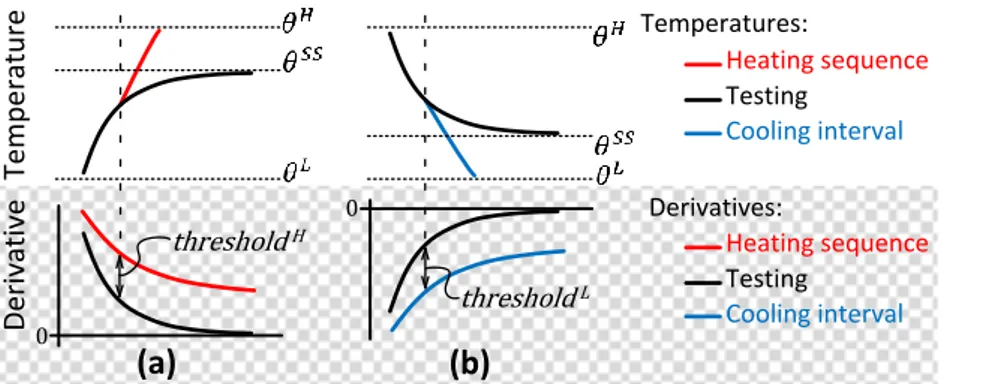
Assume that a high power test is being applied in a heating scenario as shown in Fig. 9a. Assume that the high-power test’s power for the current time interval is denoted by 𝑃𝑚𝐻𝑇. This power rapidly

increases the temperature at the beginning. Assume that this level of power is applied for a long time. In this case a steady state temperature equal to 𝜃_𝑚𝑆𝑆 will eventually be reached. As the current temperature approaches 𝜃_𝑚𝑆𝑆, the heating rate decreases. The derivative of the temperature (i.e., heating rate) is shown in the lower part of Fig. 9a. When the difference between the heating-sequence’s heating rate and the test’s heating rate increases beyond a certain threshold (𝑡ℎ𝑟𝑒𝑠ℎ𝑜𝑙𝑑𝐻

Fig. 8 An example for schedule generation. Curves are illustrative.

module m

s

s

s

s

module m

s

s

s

s

TAM

m

m

m

m

sc

h

ed

u

le

Te

st

G

ra

p

h

O

rd

er

in

g

m

m

Pause

Start/

Resume

Te

m

p

er

at

u

re

C

u

rv

es

&

N

o

d

e

Tr

an

si

ti

o

n

s

m

m

s

s

s

s

s

s

s

s

s

s

s

s

s

s

s

s

s

s

s

s

s

s

cycles

node

state

node

state

i

s

i

s

i

s

s

i

s

s

i

s

s

i

s

s

i

s

s

i

s

s

in Fig. 9a), it is time to switch to the heating sequence. This will rapidly increase the temperature to 𝜃𝑚𝐻. Temperature caused by heating sequence (shown as the red curve in Fig. 9a) introduces a heating

rate much larger than that of the test. Therefore, it is better to save the rest of the tests for a time that the initial temperature is lower and the tests can offer a large heating rate. The rate of temperature change (heating rate in this case) is 𝑑

𝑑𝑡𝜣. Therefore the condition on heating rate is: 𝑑 𝑑𝑡𝜣 𝐻𝑆₋ 𝑑 𝑑𝑡𝜣 𝐻𝑇_{> 𝑡ℎ𝑟𝑒𝑠ℎ𝑜𝑙𝑑}𝐻_. (16) The temperature when the heating sequence is applied is denoted by 𝜣𝐻𝑆_{. When the high-power test}

is applied, the temperature is denoted by 𝜣𝐻𝑇_{. The heating rate can be calculated based on the current}

temperature and upcoming power values using Equation 1:

𝑑 𝑑𝑡𝜣

𝐻𝑇 _{= 𝑨}−1_{× (𝑷}𝐻𝑇_{− 𝑩 × 𝜣}𝐻𝑇_).

(17) Combining Equation 16, Equation 17, and the equivalent of Equation 17 for the heating sequences results in:

𝑨−1_{× [(𝑷}𝐻𝑆_{− 𝑩 × 𝜣}𝐻𝑆_{) − (𝑷}𝐻𝑇_{− 𝑩 × 𝜣}𝐻𝑇_{)] > 𝑡ℎ𝑟𝑒𝑠ℎ𝑜𝑙𝑑}𝐻

(18) Considering the fact that at the moment of decision making, there is only one actual temperature, 𝜣 (𝜣 = 𝜣𝐻𝑆_{= 𝜣}𝐻𝑇_{), the condition can be further simplified to:}

𝑨−1_{× (𝑷}𝐻𝑆_{− 𝑷}𝐻𝑇_{) > 𝑡ℎ𝑟𝑒𝑠ℎ𝑜𝑙𝑑}𝐻 _.

(19) This could be re-written to have the condition expressed for the power values:

(𝑷𝐻𝑆_{− 𝑷}𝐻𝑇_{) > 𝑨 × 𝑡ℎ𝑟𝑒𝑠ℎ𝑜𝑙𝑑}𝐻 _.

(20) Renaming (𝑨 × 𝑡ℎ𝑟𝑒𝑠ℎ𝑜𝑙𝑑𝐻_{) to 𝝍 results in:}

𝑷𝐻𝑆_{− 𝑷}𝐻𝑇 _{> 𝝍 .}

(21a) Similarly, for the situation that the temperature must decrease (as shown in Fig. 9b), the proper condition for switching from a test to a cooling interval is:

𝑷𝐿𝑇_{− 𝑷̂ > 𝝋 .}

(21b) The power of the low-power test is denoted by 𝑷𝐿𝑇 _{and the power of the cooling interval (i.e., the}

stray power) is denoted by 𝑷̂. Switching to the cooling interval when indicated by the above equation speeds up the cooling. This way, the normal tests are employed in an efficient way during temperature-cycling process so that the overall test application time is further reduced.

According to Equations 21ab, the scheduling heuristic does not need to compute the derivatives of the upcoming tests’ temperatures. Instead, it is sufficient to compare the upcoming power values. Whenever the inequality in Equation 21a is satisfied, test nodes are followed by heating nodes and whenever the inequality in Equation 21b is satisfied, the testing is paused for cooling purpose. The variables 𝜓𝑚 and 𝜑𝑚 (elements that construct 𝝍 and 𝝋 vectors), are to be optimized along with 𝜃𝑚𝐻

and 𝜃𝑚𝐿, in the outer optimization loop, to achieve a short test application time. These variables are

optimized using a canonical form of particle swarm optimization similar to the one explained in Section 6. The path-graph scheduling is shown in Fig. 7 as a part of the scheduling algorithm. Since the optimization process is similar to the PSO discussed in Section 6, Fig. 7, as a whole, can be viewed as one of the scheduler boxes shown inside the dashed box in Fig. 6. The alternative decision variables shown above Fig. 7 come from Fig. 6.

Fig. 9 Thresholds in the integrated approach: (a) Heating and (b) Cooling.

(a)

(b)

7.2 Length of the Power Averaging Window

The average upcoming powers (i.e., 𝑷𝐿𝑇_{, 𝑷}𝐻𝑆_{, and 𝑷}𝐻𝑇_{) can be calculated for a short segment of the}

tests or heating sequences that immediately follows. The shortest length of this segment is denoted by 𝜆𝑚 for module 𝑚. Having a much shorter segment than 𝜆𝑚 leads to higher computational effort

without a significant improvement in the accuracy. Taking multiple 𝜆𝑚s into account helps to obtain

a long-term estimate of the power values. A much longer minimal segment length than 𝜆_𝑚 is not desirable since an accurate estimate becomes unlikely to achieve.

The proper value of 𝜆𝑚 depends on the dynamics of the system. Consider a 𝜆𝑚 that corresponds to

100𝑥 percent (0 < 𝑥 < 1) of the final response to a step input. Here, the final response is the steady state temperature and the step input is when zero input power is followed by a constant power. Assuming a constant power, the temperature equation in the time-domain can be written according to Equations 2 and 3. We assume that the step response starts from the initial temperature equal to zero (𝜽0_{= 𝟎). Replacing 𝜽}𝜏 _{with the 100𝑥 percent of the final temperature results in}

𝑥 × 𝜽𝑆𝑆_{= 𝜷(𝑡) × 𝑷 .}

(22) Since the steady state situation means negligible variations in the temperature, the temperature derivative can be assumed zero (𝑑

𝑑𝑡𝜽

𝑆𝑆_{= 𝟎). By combining this observation with Equation 1, the}

steady state temperature can be described as:

𝜽𝑆𝑆_{= 𝑩}−1_{× 𝑷 .}

(23) Replacing 𝜽𝑆𝑆 _{from the above equation and 𝜷 from Equation 3b in Equation 22 results in}

𝑥 × 𝑰 × 𝑩−1_{× 𝑷 = (𝑰 − 𝜶(𝜏)) × 𝑩}−1_{× 𝑷 .}

(24) Here we are going to replace a scalar time, 𝜏, with a matrix of time, 𝚲. Besides, we assume that the equivalence of the sides in the above equation is achieved by satisfying the following equation (Equation 25). These assumptions work for estimating the values of 𝜆𝑚’s [37].

𝑥 × 𝑰 = 𝑰 − 𝜶(𝚲) . ₍₂₅₎

Replacing 𝜶 from Equation 3a results in

exp(−𝑨−1_{× 𝑩 × 𝚲) = (1 − 𝑥) × 𝑰 . (26)}

And finally

𝚲 = 𝑩−1_{× 𝑨 × ln(1/(1 − 𝑥)) .}

(27) (𝑩−1_{× 𝑨) is the time constants matrix [37] (analogous to 𝑅𝐶 in Equations 4, 7–11, and 14 for a}

single-element case) and 𝚲 is the matrix that contains the values of 𝜆𝑚s. A diagonal element in 𝚲

(i.e., 𝜆𝑚,𝑚 that is denoted by 𝜆𝑚) represents the proper minimal length for averaging the upcoming

test powers for module 𝑚. A 𝜆𝑚’s value obtained this way is not too short and will contain the

required information. On the other hand, the use of such 𝜆𝑚 values prevents the temperature changes

that are larger than 𝑥 × 𝜃𝑚𝑆𝑆 from going unnoticed. This percentage, 𝑥, is only used for estimating

the upcoming tests’ average powers. The temperature simulations are always performed based on the original power sequence. Therefore, the value of 𝑥 will not affect them.

A set of experiments reported in [28] evaluate the accuracy of 𝜆𝑚 values estimated using Equation

27. The accurate value for 𝜆𝑚 is obtained based on high quality temperature simulations. The

average error is found to be around five percent. Besides, for 95 percent of the samples, the error is smaller than 14 percent. This confirms that the above estimates have sufficient accuracy, in practice.

7.3 Priorities for TAM Access

Normal tests, heating sequences, and cycling tests may compete for access to TAM. The priority for letting module 𝑚 to access TAM is assigned based on the following criterion.

𝜋𝑚= (𝜃𝑚𝐿 − 𝜃𝑚) ×

𝐴𝑇𝐶𝑚𝑅

𝜖 + 𝐴𝑇𝐶𝑚× 𝑟𝑚 (28)

Similar to Equation 15, the priority is higher for the colder modules and for the modules with larger remaining ATC. Moreover, a module’s priority is higher if it’s current amount of remaining tests (denoted by 𝑟𝑚) is larger. Both normal and cycling tests are taken into account for 𝑟𝑚 calculation.

The motivation for inclusion of 𝑟𝑚, similar to that of 𝐴𝑇𝐶𝑚, is to avoid a small number of modules

running long after all other modules have completed their tests. Such a scenario implies inefficient use of TAM due to lack of interleaving opportunities. In the above equation, 𝜃𝑚𝐿 is used to calculate