V¨
aster˚
as, Sweden
Thesis for the Degree of Master of Science in Engineering - Robotics
30.0 credits
A WAVELET-BASED SURFACE
ELECTROMYOGRAM FEATURE
EXTRACTION FOR HAND GESTURE
RECOGNITION
Axel Forsberg
afg13002@student.mdh.se
Examiner:
Ivan Tomasic
M¨
alardalen University, V¨
aster˚
as, Sweden
Supervisors: Sara Abbaspour
M¨
alardalen University, V¨
aster˚
as, Sweden
Nikola Petrovic
M¨
alardalen University, V¨
aster˚
as, Sweden
May 16, 2018
Abstract
The research field of robotic prosthetic hands have expanded immensely in the last couple of decades and prostheses are in more commercial use than ever. Classification of hand gestures using sensory data from electromyographic signals in the forearm are primary for any advanced prosthetic hand. Improving classification accuracy could lead to more user friendly and more naturally controlled prostheses. In this thesis, features were extracted from wavelet transform coefficients of four chan-nel electromyographic data and used for classifying ten different hand gestures. Extensive search for suitable combinations of wavelet transform, feature extraction, feature reduction, and classi-fier was performed and an in-depth comparison between classification results of selected groups of combinations was conducted. Classification results of combinations were carefully evaluated with extensive statistical analysis. It was shown in this study that logarithmic features outperforms non-logarithmic features in terms of classification accuracy. Then a subset of all combinations containing only suitable combinations based on the statistical analysis is presented and the novelty of these results can direct future work for hand gesture recognition in a promising direction.
Table of Contents
1 Introduction 1
2 Background and Related Work 3
2.1 Wavelet Transform . . . 3
2.1.1 Discrete Wavelet Transform . . . 3
2.1.2 Wavelet Packet Transform . . . 3
2.1.3 Mother Wavelets . . . 4
2.2 Feature Reduction . . . 5
2.2.1 Feature Projection . . . 5
2.2.2 Feature Selection . . . 5
3 Research Goals and Research Questions 7 4 Method 8 4.1 Data Acquisition and Preprocessing . . . 8
4.2 Wavelet Transformation . . . 8
4.3 Feature Extraction . . . 8
4.4 Normalisation . . . 9
4.5 Feature Reduction . . . 9
4.5.1 PCA . . . 9
4.5.2 ULDA and OLDA . . . 9
4.5.3 GDA . . . 11
4.5.4 mRMR . . . 11
4.6 Classification . . . 11
4.6.1 Support Vector Machine . . . 12
4.6.2 K-Nearest Neighbour . . . 12
4.6.3 Linear Discriminant Analysis . . . 12
4.6.4 Quadratic Discriminant Analysis . . . 12
4.7 Limitations . . . 12
5 Results 14 5.1 Initial Test . . . 14
5.2 Second Test: Introducing Feature Reduction Methods . . . 18
5.2.1 Separate Comparison of Logarithmic and Non-Logarithmic Features . . . . 19
5.3 Third Test: Introducing Normalisation Methods . . . 20
5.4 Fourth Test: Introducing Concatenated Features . . . 21
6 Discussion 24
7 Conclusion 26
8 Future Work 27
9 Acknowledgements 28
1
Introduction
The functionality of the human hand is crucial for performing activities of daily living with ease, such as carrying a glass of water or getting dressed. The unfortunate loss of the hand limits the ability to interact with the surroundings and may cause both physical and mental illness [1]. The most common reason for amputation of upper limb is traumatic injuries [2] obtained in for example car accidents or at war but conditions can occur already from birth.
A prosthetic hand can be used to help the impaired with daily activities. In the past decades, research publications on upper limb prostheses have increased exponentially [3]. During this pe-riod, prostheses have developed from being purely static, aesthetic devices to become complex, electronically powered bionics. Most research on prosthetic hands have been conducted with elec-tromyographic, pattern recognition control.
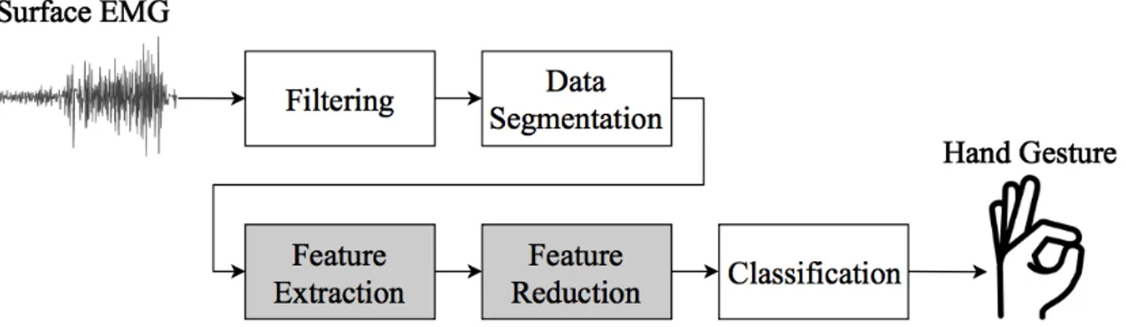
Electromyography (EMG) is a biological signal which corresponds to the electrical activity in skeletal muscles. EMG can be measured with both invasive and non-invasive techniques. The latter, usually called surface EMG (sEMG), is the most commonly used due to the absence of surgical procedures. These signals are measured with electrodes on the skin of the patient and are constructed of the algebraic sum of motor unit action potentials [4]. In pattern recognition control of prostheses, the EMG signals are mapped into different hand gestures, thus enabling the device to follow the intention of the user. This requires filtering of the measured EMG signal, data segmentation, feature extraction, and classification [5]. The general procedure of a hand motion recognition system can be seen in Figure1.
Filtering is important to be able to extract reliable information for pattern recognition. It removes unwanted interferences such as electrode noise, power line interference, and movement artefacts [6]. In the next step, data segmentation, the filtered data is divided into windows where appropriate feature extraction can be performed. Features can be calculated directly from time domain (TD), frequency domain (FD) via Fourier transform, or time-frequency domain (TFD) for example via wavelet transformation [1].
Features in TD and FD are used for analysing stationary signals, however EMG signals are non-stationary. Thus, TFD features which contain both time- and frequency information are more appropriate [7]. Wavelet based transforms are dependent of a mother wavelet function and the level of decomposition. Comparative studies on these parameters have been done in [8,9]. Features extracted from wavelet transform are often many in amount and when the feature space is large, feature reduction methods are used to relieve the classifier of heavy computational burden.
The classifier is the last part of the pattern recognition method. It is trained to classify the EMG signals of the remaining forearm into a predetermined set of different hand gestures. Popular classifiers used in hand gesture recognition are for instance Linear Discriminant Analysis (LDA) [10–12], Support Vector Machine (SVM) [8,13,14], and different types of Artificial Neural Networks (ANN) [15–17].
Although much research has been conducted on myoelectric hand prostheses, the functionality of the human hand is still unmatched. Thus, improvements in hand gesture recognition have the possibility to provide more natural control of prosthetic devices and help amputees with their daily
Figure 1: The general procedure of a hand motion recognition system. The main focus in this study is on feature extraction and feature reduction.
lives.
This study is focusing on defining and applying new configurations of EMG hand gesture recognition by proposing suitable parameters (mother wavelet and level of decomposition) for wavelet transform and finding effective dimensionality reduction.
The remainder of the thesis is structured as follows. In Section 2, the preliminaries of this study is shortly explained together with a thorough review of the state of the art of hand gesture recognition with wavelet-based features. Research goals are discussed in Section 3 and three different research questions are stated. Furthermore, in Section4, the algorithms used for each step of the hand motion recognition process is explained in detail. Test results are presented in Section5together with an explanation of the experimental process. The results are then discussed in Section6followed by concluding remarks in Section 7. Finally, interesting areas of future work are proposed in Section8.
2
Background and Related Work
This section gives the theoretical background needed to understand the thesis and provides exten-sive state of the art of hand gesture recognition with wavelet-based features.
2.1
Wavelet Transform
Signal representation in TFD is useful for non-stationary signals and wavelet transform is explicitly useful for analysis of bioelectrical signals [18]. Compared to the Fourier transform, in which a signal is represented as a sum of infinite time sinusoids of different frequencies, the wavelet transform represents a signal by coefficients related to translation and scaling of a finite time mother wavelet function. The translation can be seen as the time parameter and the scale is inversely related to frequency. That is, a higher scale means a lower frequency. Mother wavelets will be further explained in Section2.1.3.
A primitive transform to TFD is Short Time Fourier Transform (STFT), which basically is a windowed Fourier transform. This enables time-frequency analysis with a fixed resolution corre-sponding to the window length. The shorter the window, the greater time resolution but poorer frequency resolution. To overcome this problem, wavelet transform gives a multiresolutional rep-resentation of the signal [19]. This means that we can get high time resolution and low fre-quency resolution for high frefre-quency transients while still having high frefre-quency resolution and low time resolution for longer lasting low frequency components of the signal. Other than EMG feature extraction, wavelet transform has applications in signal denoising, for example EMG de-noising [20–22], and image compression [23].
2.1.1 Discrete Wavelet Transform
There are many different kinds of wavelet transforms but the most commonly used in signal pro-cessing is the Discrete Wavelet Transform (DWT) and its variants. Compared to the Continuous Wavelet Transform (CWT) the DWT is more computationally effective and much simpler to im-plement [19]. It works by filtering the signal with both a low pass filter and high pass filter which divides the frequency components of the signal into two halves. The high pass half is called detail coefficients and the low pass half is called approximate coefficients. In the filtering process the signal is also down-sampled by a factor of two, as can be seen in (1) and (2).
Approximate: y[n] = ∞ X k=−∞ x[k]g[2n − k] (1) Detail: y[n] = ∞ X k=−∞ x[k]h[2n − k] (2)
Where g and h correspond to the low and high pass filters respectively. The two filters are related as quadrature mirror filters and are derived from the mother wavelet.
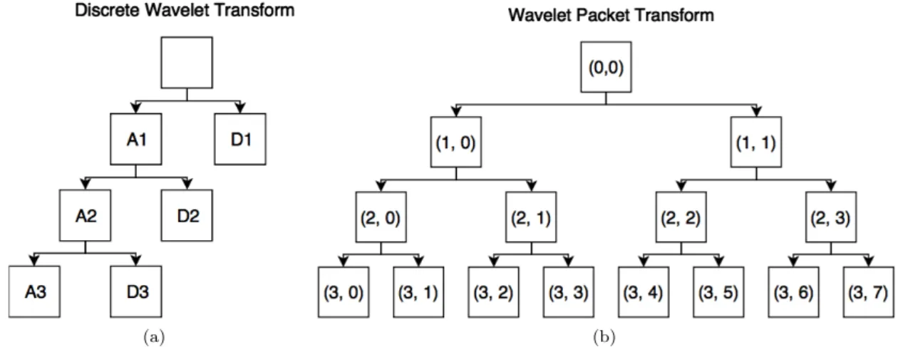
The signal is further decomposed by repeating this process recursively but only on the approx-imate coefficients. This tree structure can be seen in Figure2a.
2.1.2 Wavelet Packet Transform
The Wavelet Packet Transform (WPT), introduced by Coifman et al. [24], is a variation of the DWT. Instead of only decomposing the approximate coefficients, the decomposition is continued on both sides of the wavelet tree giving a more detailed frequency resolution for high frequencies as can be seen in Figure2b. When decomposition is done in this way, the frequency sub-bands are called wavelet packets. This allows for an even more flexible resolution analysis than in DWT.
After transformation with DWT or WPT the coefficients might be used directly as features, however this is not recommended [25]. Instead feature extraction methods originally from TD can be applied on the different frequency sub-bands from the transform. Common examples are Mean Absolute Value (MAV) and other statistical methods [14–16,26,27] and energy or entropy [7,13,
17,25,28,29]. These obtained features are often exposed to feature reduction methods to reduce computational time and increase classification accuracy.
(a) (b)
Figure 2: Different wavelet trees at decomposition level 3. In(a), A/D1 means the approximate/de-tail coefficients for decomposition level 1. In(b), the wavelet packets are numbered by (x, y) where x is decomposition level and y is packet number.
2.1.3 Mother Wavelets
The main parameters in wavelet transform are the selection of mother wavelet function and level of decomposition. The DWT sub-band filters are derived from the mother wavelet and the decom-position level determines how fine the frequency resolution is in the sub-bands. Wavelets are finite in time and have a zero mean. The zero mean property is mathematically defined in (3) [30].
Z ∞
−∞
ψ(t)dt = 0 (3)
where ψ(t) is the mother wavelet function.
Wavelets are categorised into wavelet families depending on their properties. Wavelet families useful in DWT are for example Daubechies (db), Symlets (sym), and Coiflets (coif). The simplest wavelet is the Haar wavelet which is included in the Daubechies wavelet family. It is sometimes denoted db1 which means it is the Daubechies wavelet of order 1. Haar wavelet is symmetric while other db-wavelets of higher order are asymmetric and more complex [30].
In a study by Rafiee et al. [31], investigation on the mother wavelet most similar to bioelectrical signals was performed. A similarity measure was calculated for an extensive amount of mother wavelets at fourth decomposition level and compared to three kinds of bioeletrical signals including EMG. The wavelet function found most similar was db44. If the similarity of the mother wavelet is useful in classification purposes was however left for future work.
In the purpose of feature extraction for hand motion recognition, Kakoty et al. have investigated different mother wavelets and level of decomposition with DWT [8]. The results obtained showed that sym8 wavelet at third decomposition level have statistically significant advantage over other mother wavelets. Average recognition ratio was higher for third decomposition level compared to fourth and fifth for all mother wavelets.
A continuation of their work was done by Al Omari et al. where a different set of mother wavelets and decomposition levels were used [9]. In their study, the results of two different classi-fiers was compared, SVM and a type of ANN called Probabilistic Neural Network (PNN). The PNN together with coif4 mother wavelet at sixth decomposition level produced the highest classification accuracy. In contrast to Kakoty et al. [8], results in this study indicated higher classification accu-racy with higher level of decomposition. These contradictory results motivates for more research on optimal mother wavelet and level of decomposition combination.
Karimi et al. used a different approach to select mother wavelet and level of decomposition [15]. A Genetic Algorithm (GA) was implemented and trained to select the mother wavelet function, level of decomposition, and number of hidden neurons in their ANN classifier. Using this method, the optimised wavelet chosen by the GA was db44 at fourth decomposition level. However, only
Daubechies wavelets were considered and therefore further investigation is required.
In the works by Englehart et al. they compared both DWT and WPT [11,12]. They used a coif4 mother wavelet for DWT and for WPT they used a sym5 mother wavelet. They got their best classification results when using WPT features together with Principal Component Analysis (PCA) dimensionality reduction and an LDA classifier.
2.2
Feature Reduction
When the feature space is large, as is often the case with wavelet-based features, a feature reduc-tion method can be applied to relieve the classifier of heavy computareduc-tional burden and improve classification results [5]. Feature reduction methods can be categorised as feature projection and feature selection methods. The difference between feature projection and feature selection is that in feature projection, the full feature set is transformed into a smaller dimension, whereas in fea-ture selection, there is an algorithm that chooses the most appropriate feafea-tures from the original feature set [32]. Feature projection has been used much in research of EMG pattern recognition with wavelets [14,16,17,26,33].
2.2.1 Feature Projection
Feature projection methods transform the feature space such that the features can be sorted for example by their variance or discriminative ability. Two methods for feature projection are unsupervised with PCA and supervised with LDA. In PCA, the features are sorted according to the variance of the transformed features and then features can be selected to contain for instance 90% of the total variance and the rest can be discarded. With LDA, the features are instead sorted by discriminative ability [32].
In the work by Englehart et al. [11,12] they showed that feature projection with PCA gives better classification results than feature selection with a Euclidean distance class separability cri-terion.
Chu et al. improved functionality of PCA, which is a linear transformation, with a non-linear Self-Organising Feature Map (SOFM) [16]. They used WPT and MAV of the coefficients as features. The PCA+SOFM method provided higher classification accuracy than with only PCA, without considerably increasing processing time. SOFM alone yielded highest classification accuracy but greatly increased processing time. That is why the feature set first is reduced by PCA and then by SOFM. Khushaba et al. argued that PCA could be further improved by having the non-linear part before PCA occurred [17]. For this purpose, SOFM can not be used and they implemented a Fuzzy C-Means (FCM) algorithm to cluster the features based on their class separability. From the clusters, only the features that contributed to the classification was selected and further reduced by PCA. They used WPT with energy of the packets as features and an MLP classifier.
In another work by Chu et al., a supervised feature projection method was evaluated [26]. An LDA based feature projection method was implemented and outperformed both PCA and SOFM in processing time and classification accuracy.
Zhang et al. also compared performance of PCA and LDA feature extraction and they came to the same conclusion that LDA outperforms PCA [33]. They also implemented another approach combining the two methods for which the result did not improve much compared to using only LDA. They implemented this on a real prototype prosthetic hand with an MLP as classifier. It showed promising real-time results for hand gesture recognition.
2.2.2 Feature Selection
Although feature selection was outperformed by PCA [11,12] it has been used in a few publications. Wang et al. have used a genetic algorithm (GA) for reducing the feature space after a so called harmonic WPT [29]. They used energy of the coefficients and an ANN classifier. They trained the GA by giving feedback from the classifier. After the GA had found optimal feature selection the ANN classifier was trained again with these features.
In the work of Xing et al. [7], feature selection is used in combination with feature projection. The energy of packets from WPT were used as features and then feature selection was made based
on a discriminative criterion function. For further dimensionality reduction, the feature space were reduced with a non-parametric weighted feature extraction (NWFE) introduced by Kuo and Langrebe [34]. The NWFE method was introduced as an improvement to feature projection with LDA, however when applied to energy features from WPT, calculation of the inverse of a singular matrix occurs. To solve this problem they implemented a recursive feature selection algorithm to keep this matrix from becoming singular. This method showed promising real-time results and was deployed for controlling a virtual hand.
3
Research Goals and Research Questions
The available research on wavelet based hand motion recognition is promising but far from achieving natural control of prosthetic hands. Some of the literature show contradictory results and suggest more intensive investigation in this field.
The main purpose of this thesis was to investigate suitable hand motion recognition using wavelet-based features. Focus was concentrated on selection of mother wavelet and level of decom-position, together with appropriate methods for feature reduction. To obtain good comparative results, different classifiers were also investigated. This led to the following research questions: RQ 1: What wavelet transformation gives better classification performance, including choice of
mother wavelet and level of decomposition?
RQ 2: Which feature extraction and feature reduction method provides better classification accu-racy?
RQ 3: What combination of classifier and above mentioned parameters improves classification ac-curacy?
Improving classification accuracy might increase user-friendliness and give more natural control of prostheses. In the long run, this can help amputees when performing daily activities.
4
Method
In this thesis, an exploratory, iterative, and quantitative study investigating wavelet based feature extraction was conducted. This includes selection of mother wavelet and level of decomposition for the wavelet transform, feature extraction, appropriate feature reduction method, and classifier. The optimal combinations of mentioned components for improving classification accuracy in hand motion recognition are studied.
4.1
Data Acquisition and Preprocessing
The EMG data for this study was acquired from an open access online database called BioPa-tRec developed by Ortiz et al. [35]. There exist multiple sets of data in the database but this study considers the four channel data labelled with 10 hand motions measured from 20 able bod-ied individuals. The 10 hand motions consist of hand open/close, wrist flexion/extension, wrist pronation/supination, fine/side grip, pointer (index finger extension), and agree (thumb up).
The first step was to filter the data using conventional filtering methods, that is low-pass, high-pass, and notch filtering. Advanced filtering such as wavelet denoising is out of scope for this thesis. The filters used was Butterworth band pass filter of order 20 with cutoff frequencies 10-500 Hz was applied [36]. The 10 Hz filters out motion artefacts and removes signal offset, while the 500 Hz removes aliasing and high frequency noises. Next filtering step was to filter out the power line interference, which in Europe is at 50 Hz. This was done with a notch filter at 50 Hz.
The preprocessing part in this study refers to an offline-only procedure used to label the data. In that process, 70 % of the contraction data was labelled as the corresponding hand motion and the rest was discarded. This was done to remove part of the transient data, thus improving the training of each movement. A contraction time percentage of 70 % is recommended by Ortiz et al. [35]. Furthermore the data from pure resting is collected and added as an eleventh movement class.
After filtering and processing, a windowing function was applied to the data. An overlapping windowing technique was used so that the classifier is able to give a prediction within 300 ms, which is considered the longest acceptable delay [12]. A longer delay will result in serious usability issues due to lag between user intention and hand response. In this thesis, a window size of 200 ms was used with a 50 % window overlap, that is 100 ms window increment. This corresponds to a window length of 400 samples with 200 samples increment since sampling frequency is 2 kHz. Each window is then transformed with either DWT or WPT.
4.2
Wavelet Transformation
As mentioned in Section2 the main parameters of wavelet transformation are the mother wavelet and level of decomposition. Six different mother wavelets used in the state of the art, along with a less explored mother wavelet of the Fejer-Korovkin (fk) wavelet family were tested. The chosen mother wavelets were db2 [37], db7 [38], sym5 [11,12], sym8 [8], coif4 [9,11,12], and fk wavelet of order 22. To minimise border distortions of the transformation, Matlab uses border extension methods. Default is symmetric half point extension but in this thesis it is changed to periodic extension. The investigated levels of decomposition are 3-6, since no decomposition level lower than three or greater than six was found in the state of the art.
4.3
Feature Extraction
For DWT, coefficients in the last level of decomposition are used when extracting features as suggested by Kakoty et al. [14]. Since it is not suitable to use wavelet coefficients directly as a feature set, feature extraction methods were applied to the coefficients. This results in four features per window, meaning one feature per channel and window.
When WPT is used, the coefficients of each of the last level packets are used for extracting features. In any decomposition level of the WPT there are 2N packets, where N is the level of decomposition. With four channel data and the same extraction as in DWT, this gives 4 ∗ 2N features for each window.
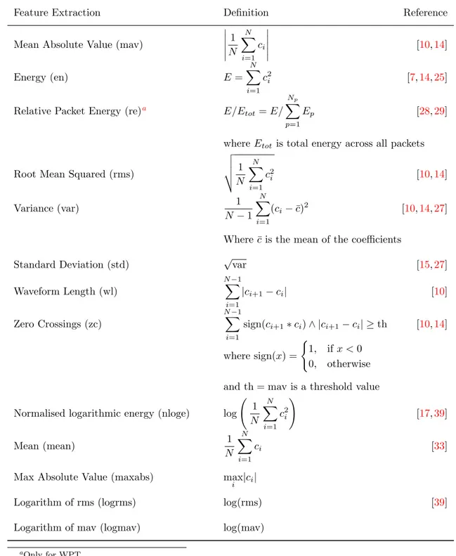
The implemented feature extraction methods were MAV and Energy based features, along with other methods usually applied in time domain. A list of implemented features is available in Table1
with accompanying mathematical definitions.
4.4
Normalisation
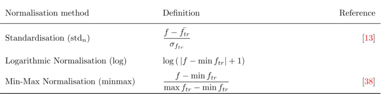
Normalisation of the features are implemented to further generalise the results from the classifier. Three different normalisation methods were implemented. Gaussian standardisation of variables (stdn), logarithmic normalisation (log), and scaling the data between 0-1 called min-max normal-isation (minmax). The subscript n stands for normalnormal-isation to distinguish stdn from std which is standard deviation feature extraction. Also classification without any normalisation was tested. This is denoted in the results as none. Mathematical definitions of normalisation methods can be found in Table2.
4.5
Feature Reduction
After the data was normalised, the feature space was reduced by a feature reduction algorithm. Both feature projection and feature selection methods have been implemented. One unsupervised feature projection method which is PCA, and three supervised LDA based feature projection meth-ods, Uncorrelated LDA (ULDA), Orthogonal LDA (OLDA), and Generalised Discriminant Anal-ysis (GDA). As feature selection method Minimum Redundancy Maximum Relevance (mRMR) is implemented.
4.5.1 PCA
The PCA is unsupervised and requires only the training data to construct a transformation matrix. The data is first centred at zero mean, then the eigenvectors of the covariance matrix of the training data are sorted in descending order of the corresponding eigenvalues. These eigenvectors are called principal components and are in the order of explained variance [33].
The first n eigenvectors will constitute the transformation matrix which reduces the feature vector to n features. In this thesis, the first 20 eigenvectors are used just as in the works of Engelhart et al. [11,12]. The eigenvectors are normalised so that each vector has unit length. This is done so that no feature is scaled in transformation.
When transforming the test data, the mean of the training data is first subtracted from each sample, then multiplied with the transformation matrix.
4.5.2 ULDA and OLDA
ULDA and OLDA feature reduction are both LDA-based feature projection methods. LDA is similar to PCA but instead of focusing on the explained variance, the reduced feature set is created to separate the classes in the best way. It does this by adding class labels for each training sample and thus is a supervised method. It finds a transformation matrix that maximises the between class scatter and minimises the within class scatter [40].
In all LDA-based feature reduction methods the maximum number of features in the reduced space is Number of classes − 1 which in this case is 10 [41]. Since it is not possible to have 20 as in the PCA reduction, the number of features for all LDA based features are 10 in this study. Computing the transformed data requires multiplication with the transformation matrix. The transformation matrices are just as in the PCA implementation normalised to unit vector length in each column.
ULDA is equivalent to regular LDA feature reduction when the within class scatter matrix (SW) is non-singular [41]. In our case this is mostly the case except for in special circumstances. Non-singular SW usually occurs in undersampled data, that is data with more features than training samples. Classical LDA cannot handle singular SW but in the ULDA implementation made by Ye et al. they calculate the transformation matrix in an effective way which also avoids the singularity problem [42]. ULDA is hence more stable than regular LDA and was therefore chosen for this work. A continuation of their implementation giving orthogonal feature vectors in the reduced space is called OLDA [43]. In OLDA a final step is added to the ULDA scheme where QR-decomposition
Table 1: Feature extraction methods applied to DWT or WPT coefficients ci. Where N is the amount of approximate coefficients for DWT and the amount of coefficients in each packet for WPT.
Feature Extraction Definition Reference
Mean Absolute Value (mav)
1 N N X i=1 ci [10,14] Energy (en) E = N X i=1 c2i [7,14,25]
Relative Packet Energy (re)a E/E
tot= E/ Np X
p=1
Ep [28,29]
where Etotis total energy across all packets
Root Mean Squared (rms)
v u u t 1 N N X i=1 c2 i [10,14] Variance (var) 1 N − 1 N X i=1 (ci− ¯c)2 [10,14,27] Where ¯c is the mean of the coefficients
Standard Deviation (std) √var [15,27]
Waveform Length (wl) N −1 X i=1 |ci+1− ci| [10] Zero Crossings (zc) N −1 X i=1
sign(ci+1∗ ci) ∧ |ci+1− ci| ≥ th [10,14]
where sign(x) = (
1, if x < 0 0, otherwise and th = mav is a threshold value Normalised logarithmic energy (nloge) log 1
N N X i=1 c2i ! [17,39] Mean (mean) 1 N N X i=1 ci [33]
Max Absolute Value (maxabs) max
i |ci|
Logarithm of rms (logrms) log(rms) [39]
Logarithm of mav (logmav) log(mav) aOnly for WPT
Table 2: Normalisation methods for wavelet features where f is an original feature, either test or training, and ftrdenotes features in the training set. Mean and standard deviation are denoted as
¯
f and σf respectively.
Normalisation method Definition Reference
Standardisation (stdn)
f − ¯ftr σftr
[13] Logarithmic Normalisation (log) log ( |f − min ftr| + 1)
Min-Max Normalisation (minmax) f − min ftr max ftr− min ftr
[38]
of the transformation matrix in ULDA is calculated. The Q-matrix from that calculation is then the OLDA transformation matrix producing orthogonal feature vectors.
4.5.3 GDA
LDA is based on linear separation between classes, just as ULDA and OLDA. To extend it to non-linear separation, the kernel trick can be used. This is called Generalised Discriminant Analysis (GDA). GDA uses a kernel function to map the data into a higher dimensional space where the classes might be linearly separable [44]. Matlab implementations of GDA can be found in [45] and in van der Maaten’s feature reduction toolbox [46]. A combination of these two implementations was used in this thesis. A Gaussian or Radial Basis Function (RBF) kernel function with parameter r = 1 was used for GDA feature reduction in this project. The number of features used in this study was 10.
4.5.4 mRMR
Feature selection was implemented with mRMR. Peng and Ding have implemented mRMR in Matlab but it works only for categorical/discrete input data [47,48]. The EMG data is continuous and thus requires discretisation of the training data. This is done by distributing the input data into 100 discrete bins of equal size. After mRMR have been applied on the discretised training data the selected features are then extracted from the original training data and testing data. The Mutual Information Quota (MIQ) scheme of the mRMR was used instead of Mutual Information Difference (MID) as recommended in [48]. The number of features selected with mRMR is variable but 20 was used in this study to be consistent with PCA reduction.
4.6
Classification
The final part in the hand gesture recognition is the classification. To evaluate classification performance, a k-fold cross-validation scheme was implemented. In this thesis K = 10. This means that the data is randomly divided into ten equally large parts or folds. Initially the first fold is used as test data and the remaining nine folds are used for training. This is then repeated with the next fold as test data and the rest as training data, until all folds have been the test data. Classification accuracy is calculated for each fold as the number of correctly classified windows divided by the total number of windows. The reported classification accuracy is then the mean of the accuracy from the ten different folds. This procedure is done to generalise the classification and to make sure the classifier is not overtrained. Normalisation and feature reduction are included in the k-fold cross-validation and takes place right before the classification.
To increase the credibility and reliability of the classification results, in-depth statistical analysis was performed to find statistical significance between different groups of combinations. In all statistical tests, a significance level of 0.05 was used.
When more than two groups were compared, a one-way analysis of variance (ANOVA) test was deployed to examine whether any group had a different mean than the others. Then a post hoc
test with Tukey’s Honest Significant Difference criterion (HSD) was used. This determines which groups that differ from each other by comparing each group to all other groups individually.
When exactly two groups are compared a t-test was used to determine whether the results in each group are statistically different from each other.
The data is not mixed between subjects, which means the training procedure is subject de-pendent. This is commonly done in the field of hand motion recognition since the prosthesis is a highly individual accessory. Four different classifiers were implemented, SVM, K-Nearest Neigh-bour (KNN), LDA, and Quadratic Discriminant Analysis (QDA). MLP was considered but left out due to large training times.
4.6.1 Support Vector Machine
An SVM classifier is a binary classifier that uses instances of each class as support vectors to create the hyperplane (linear case) that separates classes with the widest margin. Classes are not always separable and therefore a parameter C is specified such that it punishes misclassification harder the higher value it has. In this work C was set to 1. For nonlinear classification, SVM can be used with the kernel trick and in this thesis a Gaussian or RBF kernel has been used with parameter r = 1 [49].
Since SVM is a binary classifier it was extended with a one-versus-all (OVA) scheme to enable multi-class classification. This means that a binary classifier was created for each class. Samples belonging to that class are positive samples all other classes are considered negative samples. When classifying a new test sample all binary classifiers cooperates to select the output class for the multi-class classifier [50].
4.6.2 K-Nearest Neighbour
The second classifier is a classical K-nearest neighbour algorithm. When classifying a new test sample it finds the K points of the training data with the shortest euclidean distance to the test sample. In this case, K = 4. It then classifies the test sample as the class that includes the most of the neighbouring points. If tied, the class of the nearest neighbour is chosen.
4.6.3 Linear Discriminant Analysis
LDA is a robust, fast, and easy to use classifier. There are certain differences when LDA is used as a classifier compared to a feature reduction method. In the classifier the objective is to minimise a classification cost function that calculates the Gaussian posterior probability of an observation x belonging to class c. This is under the assumptions that all classes share the same covariance matrix [51].
In Matlab there are two parameters that can be altered, δ and γ. These parameters control the level of regularisation, δ is a threshold that removes LDA coefficients which are less than δ, while γ is a proper regularisation parameter that alters regularisation of the covariance matrix. These parameters were both set to Matlab default value zero in this study.
4.6.4 Quadratic Discriminant Analysis
QDA is a non-linear version of regular LDA where covariance matrix may differ between classes. In this particular implementation the covariance matrices are inverted using the pseudo inverse to avoid singularity problems. This results in quadratic separation instead of linear as in LDA. The same parameters as in LDA was used for QDA [51].
4.7
Limitations
As previously discussed in Section1and2, there is a lot of research in the area of robotic prosthetic hands. Therefore, this study is focusing on wavelet-based feature extraction and dimensionality reduction on sEMG signals for hand gesture recognition. Filtering and windowing was used but are not the main focus of this thesis.
This study has used pre-recorded data, which means true online classification has not been performed. Also, no physical prototype of a prosthetic hand was used. Thus, classification was the last step of the hand motion recognition scheme and no motor control was considered.
5
Results
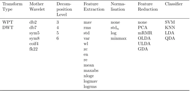
The possible combinations from everything in Section4consist of different values of seven variables. These correspond to two types of wavelet transform, six mother wavelets, four different decom-position levels, 13 feature extraction methods, four normalisation methods, six feature reduction methods, and four classifiers, which gives a total of 2 ∗ 6 ∗ 4 ∗ 13 ∗ 4 ∗ 6 ∗ 4 = 59904 combinations. These combinations are listed in Table3. To test them all is infeasible, thus, the testing procedure is divided into four tests where the results of one test set the premises for the next test. This leads to more efficient search to find suitable combinations.
The combinations were compared one on one to see which combination had highest accuracy but also compared in groups to get more general results. In these more general comparisons, groups were extracted in the following way. The set of combinations was restricted to contain only one value for one of the variables, for example the variable ’classifier’ can be set to SVM. Then the classification results of all the combinations containing SVM classifier was extracted with no regard to values of other variables (if nothing else is stated). The results were sorted according to their classification accuracy and the top 50 % constitute the group. Using only the top 50 % was to minimise the effect of the worst combinations for each value of a variable. This process was then repeated for all groups before being compared in a statistical test.
All tests were done on a PC with Windows 10, an Intel CoreR TM i7-4510U @ 2.00 GHz processor, and 8 GB RAM.
5.1
Initial Test
Since the total set of combinations was too large to test all combinations explicitly, the first test did not consider different normalisation methods or feature reduction methods. Only one normalisation method was chosen and only one reduction method. Trial and error suggested that stdn as normalisation and OLDA as feature reduction was a good starting point. The other normalisations and reduction methods were to be included in future tests. Feature reduction was only used for WPT since DWT gives only four features. Also the feature re is not applicable for DWT since it measures relative energy between packets. Instead of re, en was used for DWT. Together this gives a total of 2304 combinations that were investigated in the initial test. These combinations are listed in Table4.
The classification results of all combinations in the initial test are sorted according to their accuracy and presented in a table. Because of limited space not all 2304 combinations are presented in the paper but only the top 20 results, which are shown in Table5. Each combination is tested on all 20 subjects and the mean accuracy and standard deviation of the subjects are reported. The reported training time is the total training time across all K-folds and all subjects while the reported execution time is the average execution time of each time window.
Note that all results in the table come from combinations with WPT as transform type. In fact the top 517 combinations had WPT as transform type. Comparison of the groups of WPT and DWT showed that the mean accuracy of WPT (0.9433 ± 0.0478) was significantly higher than that of DWT (0.7656 ± 0.1262), (p < 0.001). Because of this large and significant difference, further analysis of this test does not consider DWT.
Furthermore, significant differences was found between different levels of decomposition by an ANOVA test (p < 0.001). The accuracies of decomposition levels three (0.9540 ± 0.0370) and four (0.9528 ± 0.0416) were significantly higher than decomposition levels five (0.9422 ± 0.0510) and six (0.9048 ± 0.0765).
Comparison of the six different mother wavelets showed significant difference in accuracy (p < 0.001). Furthermore it was shown that fk22 mother wavelet had significantly higher accuracy than db2, sym8, and coif4 but no significant difference between fk22, db7, and sym5 was found. Complete results of the post hoc test can be found in Table6.
A similar test was done to compare performance between features. The test proved significant differences between the features (p < 0.001). Post hoc investigation showed that logarithmic features, nloge, logmav, and logrms, had significantly higher mean accuracy than the rest of the features. Features std, mav, rms, and wl had significantly higher accuracy than the rest of the non-logarithmic features. This is shown visually in Figure3.
Table 3: List of all possible combinations based on the implemented methods in Section4. Transform Type Mother Wavelet Decom-position Level Feature Extraction Norma-lisation Feature Reduction Classifier
WPT db2 3 mav none none SVM
DWT db7 4 rms stdn PCA KNN
sym5 5 std log mRMR LDA
sym8 6 var minmax OLDA QDA
coif4 wl ULDA fk22 zc GDA en re mean maxabs nloge logmav logrms
Table 4: List of combinations in the initial test. Compared to the original set, normalisation methods and feature reduction have been reduced.
Transform Type Mother Wavelet Decom-position Level Feature Extraction Norma-lisation Feature Reduction Classifier WPT db2 3 mav stdn OLDA SVM DWT db7 4 rms none KNN sym5 5 std LDA
sym8 6 var QDA
coif4 wl fk22 zc en re mean maxabs nloge logmav logrms
Table 5: The top 20 results of combinations in the initial test. Feature reduction method was OLDA for WPT and none for DWT while normalisation was stdn for both.
Accuracy Std Type Dec Mother Wavelet
Feature Classifier Training Time (s) Execution Time (s) 0.9777 0.0186 WPT 4 fk22 nloge SVM 33.6 0.056 0.9773 0.0185 WPT 4 fk22 logrms SVM 33.5 0.056 0.9765 0.0201 WPT 4 sym8 nloge SVM 34.9 0.056 0.9765 0.0207 WPT 4 fk22 logmav SVM 34.0 0.056 0.9762 0.0230 WPT 4 sym5 nloge SVM 33.4 0.056 0.9762 0.0190 WPT 4 fk22 nloge KNN 6.19 0.054 0.9756 0.0228 WPT 4 db7 nloge SVM 35.3 0.056 0.9753 0.0210 WPT 4 db7 logrms SVM 35.0 0.060 0.9753 0.0232 WPT 4 sym5 logmav SVM 33.6 0.060 0.9751 0.0213 WPT 4 sym8 logrms SVM 36.3 0.055 0.9751 0.0242 WPT 4 sym5 logrms SVM 33.4 0.056 0.9750 0.0200 WPT 3 db7 logrms SVM 31.4 0.054 0.9750 0.0210 WPT 4 fk22 logmav KNN 6.25 0.044 0.9748 0.0233 WPT 4 sym8 logmav SVM 35.5 0.056 0.9746 0.0220 WPT 4 coif4 logmav SVM 35.2 0.056 0.9745 0.0199 WPT 3 coif4 logmav SVM 31.1 0.041 0.9743 0.0223 WPT 4 fk22 logrms KNN 6.25 0.056 0.9742 0.0208 WPT 3 db7 nloge SVM 31.4 0.044 0.9741 0.0197 WPT 3 coif4 logrms SVM 31.4 0.041 0.9741 0.0247 WPT 5 fk22 logmav SVM 34.9 0.085
Table 6: The Tukey HSD post hoc test of comparison between different groups of mother wavelets. The Significance column shows all mother wavelets that the corresponding wavelet is significantly better than.
Reduction Method Mean Accuracy Standard Deviation Significance
1 fk22 0.9474 0.0451 4-6 2 sym5 0.9458 0.0467 5-6 3 db7 0.9439 0.0476 6 4 coif4 0.9418 0.0489 5 sym8 0.9413 0.0488 6 db2 0.9390 0.0501
Figure 3: Visualisation of post hoc comparisons. Circles represent the mean accuracy for each feature type while the intersecting line shows the corresponding 95 % confidence interval. Features mean (0.2824 ± 0.0887) and zc (0.5412 ± 0.1354) have means lower than 0.8 and are left outside the figure boundaries. The dashed lines are extensions of the endpoints of the 95 % intervals of features mav and nloge respectively. Overlapping intervals indicates non-significant result in the post hoc test.
Table 7: Mean execution time for different decomposition levels. Decomposition Execution Time (ms)
3 42
4 56
5 84
6 138
Comparison of classifiers SVM, KNN, LDA, and QDA gave significant differences in accuracy (p < 0.001). It was shown that LDA (0.9311 ± 0.0522) had significantly worse results than the other classifiers by the post hoc test. Between SVM (0.9481 ± 0.0464), KNN (0.9476 ± 0.0452), and QDA (0.9462 ± 0.0453), the test indicated no significant difference.
When investigating execution time of the different combinations it can be seen that the trans-formation part contributes the most to the execution time. For example in the top result of Table5, the total execution time is 56 ms while the execution time for the transformation is 50 ms. This corresponds to 90 % of the total execution time. An ANOVA test was conducted to see if there were any differences between the different decomposition levels (p < 0.001). Post hoc test showed significant differences between all decomposition levels and higher decomposition levels increase execution time. This can be seen in Table7.
All combinations with decomposition level 6 and WPT had an execution time greater than 130 ms which is considered too slow for the hand motion recognition system. Since the window increment is 100 ms, execution time must be below that to keep up with the predictions.
Taken together, these tests indicate that features based on WPT provides higher classification accuracy than features based on DWT. Decomposition levels 3 and 4 also gave higher accuracies compared to decomposition levels 5 and 6. The mother wavelet fk22 gave higher accuracy than db2, sym8, and coif4. Logarithmic features have higher accuracy than non-logarithmic features. The best non-logarithmic features are mav, rms, std, and wl. Among classifiers, LDA showed
Table 8: List of selected combinations in the second test. Transform Type Mother Wavelet Decom-position Level Feature Extraction Norma-lisation Feature Reduction Classifier WPT db7 3 mav stdn none SVM sym5 4 rms PCA KNN fk22 std mRMR QDA wl ULDA nloge OLDA logmav GDA logrms logstd logwl
Table 9: Results of the different feature reduction methods. The Significance column shows all reduction methods that the corresponding method is significantly better than.
Reduction Method Mean Accuracy Standard Deviation Significance
1 OLDA 0.9717 0.0233 3-6 2 ULDA 0.9715 0.0234 3-6 3 mRMR 0.9645 0.0267 4-6 4 PCA 0.9525 0.0346 5-6 5 none 0.9416 0.0402 6 6 GDA 0.9093 0.0763
lower accuracy than the other classifiers. Also execution time increased significantly with the decomposition level.
5.2
Second Test: Introducing Feature Reduction Methods
In the second test, all feature reduction methods were introduced to the set of combinations. The rest of the set was selected based on the results from the initial test. Since WPT showed better accuracy than DWT, only WPT was considered. The decomposition levels chosen were 3 and 4 since they had significant advantage over decomposition levels 5 and 6.
The features selected were the logarithmic features and the top non-logarithmic features. Both logarithmic and non-logarithmic features were selected to get diversity in the combinations. Since the logarithmic features showed promising results, more logarithmic features were added. These were logarithm of std (logstd) and logarithm of wl (logwl) such that all non-logarithmic features in the set had a corresponding logarithmic feature.
Normalisation method was kept as stdn in accordance with the initial test and all classifiers except LDA, which had worse results than the others, was selected. All five reduction methods mentioned in Section4were included together with a sixth method which was no feature reduction. This is labelled as none in the results. The complete set of combinations is displayed in Table8.
A one way ANOVA test was performed to investigate if there were any differences between ac-curacy of different features (p < 0.001). The post hoc test showed that all logarithmic features were again significantly better than their non-logarithmic counterparts. This is depicted in Figure4. It is clear from the figure that logarithmic features outperform non-logarithmic features.
Significant differences between reduction methods were found when comparing (p < 0.001). It was shown that ULDA and OLDA are significantly better than the other reduction methods. These results are presented in Table9.
Comparing classifiers SVM (0.9610±0.0331), KNN (0.9612±0.0304), and QDA (0.9596±0.0318) gave no significant difference in accuracy when performing ANOVA (p = 0.094).
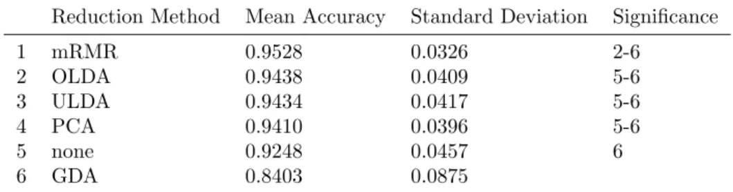
Figure 4: Post hoc results of feature comparison in the second test. Circles represents mean accuracy for each feature and the intersecting line shows the corresponding 95 % confidence interval. Overlapping intervals suggest non-significant differences between the mean accuracy of the features. Table 10: Results of the different feature reduction methods when only non-logarithmic features were considered. The Significance column shows all reduction methods that the corresponding method is significantly better than.
Reduction Method Mean Accuracy Standard Deviation Significance
1 mRMR 0.9528 0.0326 2-6 2 OLDA 0.9438 0.0409 5-6 3 ULDA 0.9434 0.0417 5-6 4 PCA 0.9410 0.0396 5-6 5 none 0.9248 0.0457 6 6 GDA 0.8403 0.0875
accuracy than non-logarithmic features. For feature reduction, OLDA and ULDA was generally giving higher classification accuracy than other feature reduction methods. This test could not significantly show any difference in accuracy between classifiers.
5.2.1 Separate Comparison of Logarithmic and Non-Logarithmic Features
Features were divided in logarithmic and non-logarithmic features. Combinations have been stud-ied with all features together not differentiating between the two distinct groups. When studying these two groups separately, different results were produced. When the set of combinations was re-stricted to only contain non-logarithmic features, comparison of reduction methods gave significant difference of the means (p < 0.001). The post hoc test then indicated that mRMR was significantly better than ULDA and OLDA, which differs from the test when all features were considered. The complete result is shown in Table10.
Comparing the three classifiers showed significant difference unlike when all features were con-sidered (p < 0.001). It was shown that KNN (0.9464 ± 0.0385) and QDA (0.9442 ± 0.0387) where both significantly better than SVM (0.9370 ± 0.0437). The difference between KNN and QDA was however not significant.
The original set of combinations was then restricted to contain only logarithmic feature ex-traction methods and the same comparison approach was conducted. Between different feature reduction methods, difference in the means was significant (p < 0.001) and the post hoc test
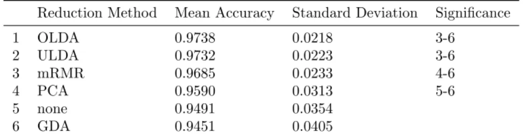
Table 11: Results of the different feature reduction methods when only logarithmic features were considered. The Significance column shows all reduction methods that the corresponding method is significantly better than.
Reduction Method Mean Accuracy Standard Deviation Significance
1 OLDA 0.9738 0.0218 3-6 2 ULDA 0.9732 0.0223 3-6 3 mRMR 0.9685 0.0233 4-6 4 PCA 0.9590 0.0313 5-6 5 none 0.9491 0.0354 6 GDA 0.9451 0.0405
Table 12: List of selected combinations in the third test. Transform Type Mother Wavelet Decom-position Level Feature Extraction Norma-lisation Feature Reduction Classifier
WPT db7 3 mav none none SVM
sym5 4 rms stdn mRMR KNN
fk22 logmav log ULDA QDA
logrms minmax OLDA
showed that OLDA and ULDA were significantly better than the other methods. In Table11, the complete result of the post hoc test is reported.
Comparing classifiers also gave significantly different results (p < 0.001). A post hoc test indicated that an SVM classifier (0.9723 ± 0.0223) had significantly higher accuracy than KNN (0.9688 ± 0.0245) and QDA (0.9670 ± 0.0264). Between KNN and QDA, no significant difference was found.
These results combined suggest that an SVM classifier is preferred when features are logarith-mic, while for non-logarithmic features either KNN or QDA should be considered instead. Also feature reduction method could be related to the feature extraction properties. For logarithmic features, OLDA and ULDA feature reduction outperformed other methods just as when all features were considered, while non-logarithmic features got better accuracy with mRMR feature reduction.
5.3
Third Test: Introducing Normalisation Methods
In the third test another set of combinations was constructed where two new normalisation methods were introduced. The previously used method stdn was kept and logarithmic normalisation (log) and normalisation between 0 and 1 (minmax) were added. Also no normalisation was used as an alternative, this is mentioned as none in the results.
The same decomposition levels and mother wavelets as in the second test were used. Since the previous tests have indicated clear separation of logarithmic and non-logarithmic features the number of selected features for this test could be reduced. For this test two of the logarithmic features were selected, logmav and logrms, and their corresponding non-logarithmic features, mav and rms, were kept to maintain diversity between the features.
Reduction methods selected for this test were ULDA, OLDA, and mRMR. No feature reduction was kept as a reference while PCA and GDA were excluded since they were significantly worse than the other feature reduction methods. All classifiers were kept since they did not have any significant difference in the previous test. All combinations are presented in Table12.
Significant difference between accuracy of the difference normalisation methods was indicated by an ANOVA test (p < 0.001). Also, no normalisation (0.9654 ± 0.0273) was shown significantly better than both log (0.9629 ± 0.0287) and minmax (0.9601 ± 0.0319) normalisation. Although, no significant difference was found between stdn (0.9645 ± 0.0286) and no normalisation.
Table 13: Results of the different normalisation methods when only SVM classifier was consid-ered. The Significance column shows all normalisation methods that the corresponding method is significantly better than.
Normalisation Method Mean Accuracy Standard Deviation Significance
1 stdn 0.9654 0.0303 3-4
2 log 0.9617 0.0295 4
3 none 0.9583 0.0413 4
4 minmax 0.9513 0.0402
Table 14: List of the concatenated features. The second column describes all features that were concatenated to constitute the corresponding vector. The third and fourth column has the total number of features in the feature vector with third and fourth decomposition level respectively.
Name Features # 3 dec # 4 dec
all (mav, rms, std, wl, nloge, logmav, logrms, logstd, logwl) 288 576
logall (nloge, logmav, logrms, logstd, logwl) 160 320
nonall (mav, rms, std, wl) 128 256
3log (nloge, logmav, logrms) 96 192
mav+logmav (mav, logmav) 64 128
rms+logrms (rms, logrms) 64 128
non+log (mav, rms, logmav, logrms) 128 256
QDA (p < 0.001). The following post hoc test indicated that KNN (0.9654 ± 0.0268) was signifi-cantly better than both QDA (0.9622 ± 0.0303) and SVM (0.9613 ± 0.0326). Between QDA and SVM there was no significant difference.
By restricting the set of combinations to contain only one of the classifiers at the time, both normalisation and classifier can be investigated. When the set was restricted to contain only SVM classifier, a one way ANOVA showed significant differences between the mean accuracy of the different normalisation methods (p < 0.001). A Post hoc using Tukey HSD algorithm indicated that, stdn was significantly better than no normalisation. A more detailed result from the post hoc is shown in Table13.
Unlike the case with SVM, when restricted to KNN or QDA, there were no significant difference between normalisation methods. The corresponding p-values were (p = 0.950) and (p = 0.250) respectively.
5.4
Fourth Test: Introducing Concatenated Features
In the fourth test, the results when features were working together was investigated. The feature vectors from different features were concatenated into larger feature sets. First, all nine features from the second test were concatenated. Then all logarithmic features were concatenated into one feature set and all non-logarithmic features to another. These feature sets got very large and some smaller sets were also created. Three logarithmic features, nloge, logmav, and logrms, constitute one of them and then three combined logarithmic/non-logarithmic feature sets were created. A list of the concatenated features is found in Table14.
All reduction methods and classifiers from the previous test were kept and as normalisation method stdn was selected since it was not significantly worse than any other method. A list of all the combinations tested is found in Table15.
The result of each of the concatenated features were compared and showed significant difference between the feature sets in an ANOVA test (p < 0.001). A post hoc test showed that mav+logmav and rms+logrms were significantly superior to all other feature sets except 3log. The complete result of the post hoc test can be seen graphically in Figure5.
These feature sets were then compared against the original single features from the second test to see if any significant improvements can be found. To compare features from the second test the
Table 15: List of selected combinations in the test with normalisation methods. Transform Type Mother Wavelet Decom-position Level Feature Extraction Norma-lisation Feature Reduction Classifier WPT db7 3 all stdn none SVM sym5 4 logall mRMR KNN
fk22 nonall ULDA QDA
3log OLDA
mav+logmav rms+logrms non+log
Figure 5: Post hoc results of comparison of concatenated features. Circles represents mean accu-racy for each feature and the intersecting line shows the corresponding 95 % confidence interval. Overlapping intervals suggest non-significant differences between the mean accuracy of the features.
Figure 6: Post hoc results when comparing both concatenated and single features. Circles rep-resents mean accuracy for each feature and the intersecting line shows the corresponding 95 % confidence interval. Overlapping intervals suggest non-significant differences between the mean accuracy of the features. Dashed lines are connected to features nonall, all, and mav+logmav to make it easier to distinguish significant difference between features.
reduction methods PCA and GDA were excluded since they were not used in this test. Comparing the features in an ANOVA test indicated significant differences (p < 0.001). The results of the post hoc test is shown in Figure6.
In the figure, it can be seen that mav+logmav and rms+logrms were significantly better than logwl but not significantly better than the other single logarithmic features. The single logarithmic features were significantly better than the all feature. Also nonall was significantly better than wl but not significantly better than the other single non-logarithmic features.
Taken together, the concatenated features are generally not improving the result significantly compared to having single features.
Another interesting result was found when comparing classifiers on the concatenated features. An ANOVA test showed that significant differences between the classifiers exist (p = 0.010) and the post hoc test showed that KNN (0.9663 ± 0.0268) was significantly better than SVM (0.9634 ± 0.0280). No significant difference between KNN and QDA 0.9648 ± 0.0285 was found.
The set of combinations was then restricted to only contain no feature reduction and sifiers are compared in an ANOVA test. The test indicated significant difference between clas-sifier accuracy (p < 0.001). Post hoc test showed that SVM had a very low classification ac-curacy (0.6838 ± 0.1473) which is significantly worse than both KNN (0.9532 ± 0.0335) and QDA (0.9380 ± 0.0412). When restricting the set to only contain the other reduction methods, mRMR, ULDA, and OLDA, the classifiers show no significant difference in classification accuracy (p = 0.1913).
Execution time naturally increased when features were concatenated and a combination of all features, decomposition level 4, and mother wavelet db7 produced execution times above 100 ms.
6
Discussion
The results presented in Section5should be interpreted carefully. For example the execution time, which needs careful programming on a real time OS to be 100 % accurate.
The execution time measured in this study is although useful since it is averaged across a lot of measurements. Also relative comparisons should be fair since all results were calculated in the same way.
When comparing accuracy between groups of features for example, one should keep in mind that the accuracy is a generalised accuracy across other variables in the combinations such as mother wavelet and level of decomposition. The results of features might be dependent of these other variables. This problem is reduced by only comparing the top 50 % results in each category, so that bad results from dependent variables are discarded.
The parameters in implementation were chosen by trial and error. Thus, careful tuning of the parameters could possibly improve the results.
In the initial tests it was stated that combinations with WPT provide better classification accuracy than DWT. This is consistent with the result of Englehart et al. [11,12]. In this thesis, no more tests included DWT because of the significant difference, however one advantage with DWT is the processing time. Since it only uses the approximate coefficients when decomposing the signal it requires a lot less computations. With WPT the number of calculations increases exponentially with the decomposition level while in DWT it increases linearly.
One of the mother wavelets with highest accuracy from the initial test was fk22. Interestingly it was the only mother wavelet not chosen from the state of the art. Although, the mother wavelet did not have a great impact on the classification accuracy. The greatest mean difference in accuracy of the mother wavelets was between fk22 and db2 (0.9474 − 0.9390 = 0.0084) which is less than 1 percentage point. This was however a significant difference. The fk22 mother wavelet had no significant difference compared to sym5 and db7. One of these three features should be recommended for use in future research.
In the initial test the decomposition levels three and four were shown significantly better than decomposition levels five and six. These results effectively answers RQ 1. WPT, decomposition level three to four, and mother wavelet fk22, sym5, or db7 should be chosen.
Looking at the spread of the results, the selection of feature extraction method had the largest difference among all variables. The mean feature had the lowest average classification accuracy (0.2824 ± 0.0887) while the logarithmic feature nloge had (0.9705 ± 0.0244). The distance is 69 percentage points. One reason that mean feature does not perform well is that the nature of the EMG signal have zero mean. The mean is not affected by the transform as seen in (3).
Also the zc feature did not have good accuracy (0.5412 ± 0.1354) however it was better than mean feature. The definition of zc contains a threshold, which in this study was set to the mean average value. Results of zc might improve by tuning this threshold value. Relative energy (re) (0.8630 ± 0.0707) was successfully used in the state of the art but in the results from the initial test it was significantly worse than a lot of features.
Apparent in both the first and second tests was that logarithmic features outperform non-logarithmic features in terms of classification accuracy (0.9694 vs 0.9434 in the second test). Also all logarithmic features had significantly higher accuracy than their non-logarithmic counterparts. This is, to the author’s knowledge, the first study that has seen tendencies of this phenomenon.
Different feature reduction methods were introduced in the second test. The LDA based meth-ods ULDA and OLDA, were significantly better than the other feature reduction methmeth-ods despite outputting a smaller feature set than in PCA and mRMR. Although when the set of combinations were restricted to only contain non-logarithmic features, mRMR outperformed both ULDA and OLDA. This suggests that feature selection with mRMR is more appropriate than the feature projection methods in this study when features are non-logarithmic. The no feature reduction was significantly better than only GDA.
Also for logarithmic features, an SVM classifier is significantly better than KNN and QDA while for non-logarithmic features the result is reversed. This suggest that logarithmic or non-logarithmic is an important property of the features which can help in selecting the correct reduction method and classifier.
Table 16: The suggested combinations for future work. Transform Type Mother Wavelet Decom-position Level Feature Extraction Norma-lisation Feature Reduction Classifier WPT db7 3 nloge stdn ULDA SVM
sym5 4 logmav OLDA KNN
fk22 logrms QDA
logstd logwl
accuracy than LDA. LDA was also the only linear classifier in the test and thus the non-linear classifiers proved better results. Between the non-linear classifiers there was no significant difference in classification accuracy. Also in the second test there was no significant difference between these classifiers unless there were other restrictions on the set of combinations.
However, in the third test where all normalisation methods were introduced, a significant increase in accuracy was found between KNN and the other classifiers. This could indicate that KNN, is more stable for different normalisation methods. Restricting the data to only include SVM classifier indicated significant difference between the normalisation methods while when restricting to the other classifiers, no significant difference was found between normalisation methods. This indicates that SVM classifier is more dependent on the choice of normalisation method than the other classifiers. The stdn normalisation was significantly better than the no normalisation when SVM classifier was used.
In the last test, the features were concatenated to see if that could increase classification accu-racy. The nonall feature did not have significantly higher accuracy than the single non-logarithmic features except for wl. The logarithmic features did not show any significant improvement when concatenated to each other but when logarithmic features were joined with their corresponding non-logarithmic feature, as in mav+logmav and rms+logrms, the results improved slightly. This improvement was only significant against logwl however. Although the execution time increased when concatenating features, these results indicates potential to improve accuracy.
Comparing the classifier performance of the concatenated features indicated that KNN was significantly better than SVM. This result can be explained by looking at only combinations with no feature reduction. Then SVM has very low classification results (0.6838 ± 0.1473). However when any of the other feature reduction methods were used the results increased to 0.9668±0.0259. This shows that SVM is more sensitive against large feature sets compared to KNN and QDA.
This result can also be reflected on the comparison of features. Since SVM does not have good performance in combination with large feature sets it is possible that this has affected the overall performance, that is when all classifiers are considered, of the largest feature sets (all and logall). The smallest concatenated features mav+logmav, rms+logrms, and 3log, were also the best performing ones which could be related to this.
With these results taken together it is possible to answer both RQ 2 and RQ 3. RQ 2 is answered easiest by selecting one of the logarithmic features together with ULDA or OLDA feature reduction. Although concatenated features mav+logmav and rms+logrms were promising they did not provide significantly better results than the logarithmic single features. Also longer execution time makes the concatenated less recommended than single logarithmic features.
Among the classifiers any of the non-linear classifiers, SVM, KNN, or QDA could be used. If SVM is used the normalisation method should be stdnwhile if any other classifier is used the choice of normalisation method does not have a significant effect on classification accuracy. Merging all results together gives the answer toRQ 3. In Table16, the most suitable combinations for future work are listed.
7
Conclusion
In this thesis, many configurations of a hand gesture recognition system with wavelet based fea-tures have been implemented and compared. The combinations consist of two transformation types, (DWT and WPT), several mother wavelets and decomposition levels, feature extraction, normalisation, feature reduction, and four classifiers. Four tests have been performed with different sets of combinations in each test. In these tests, different groups of combinations are compared and analysed with statistical methods. The tests showed that features derived from WPT had better classification accuracy than features from DWT.
Tests also showed that mother wavelets fk22, sym5, and db7 with decomposition level three and four provided higher classification accuracy than other transformations. Furthermore logarithmic features, such as logmav and logrms, tend to have higher classification accuracy than classifica-tion with non-logarithmic features. To the author’s knowledge, this is the first reported case of logarithmic versus non-logarithmic features in this domain.
Feature reduction with ULDA and OLDA outperformed other feature reduction methods in general but when non-logarithmic features were used, feature selection with mRMR resulted in the highest classification accuracy. As for normalisation methods it was shown that for SVM classifier stdn improved classification accuracy, while for KNN and QDA no significant difference in classification accuracy between normalisation methods was found.
Classification with KNN was more stable than SVM across all combinations, while SVM was included in the combinations that provided the highest classification accuracy.
8
Future Work
These result can provide a general hint in which direction future research should be taken. It is possible to both widen the search among combinations and move forward towards online classi-fication of hand gestures. Although many combinations have been compared in this thesis it is possible to extend the research to include more mother wavelets and more classifiers for example. Also classifier parameters could be investigated further.
Investigation of relationships between combinations is only done briefly in this thesis and should be done more thoroughly to further explain reasons behind certain results. For example to explain why logarithmic features provided better classification accuracy than non-logarithmic features.
The suitable combinations listed in Table 16 have promising real-time potential and can be further analysed with online classification. Furthermore, the hand gesture recognition scheme can be implemented on a real prototype prosthetic hand.
9
Acknowledgements
I would like to express my great appreciation to my supervisors Sara Abbaspour and Nikola Petrovic for their enthusiasm, guidance and helpful comments. Additionally I would like to thank my lovely girlfriend who always lighten up my day. I would like to thank my family and friends for believing in me by giving their endless support.