EVALUATION OF A SUCTION
PYROMETER
By analytical heat transfer methods
SEBASTIAN ZETTERSTRÖM
Akademin för ekonomi, samhälle och teknik Kurs: Examensarbete Kurskod: ERA403 Ämne: Energiteknik Högskolepoäng: 30 hp Program: Civilingenjörsprogrammet i energisystem
Handledare: Jan Sandberg Examinator: Ioanna Aslanidou
Uppdragsgivare: Konstantinos Kyprianidis, EST Datum: 2017-09-18
E-post:
ABSTRACT
Sebastian Zetterström, Master of Science in energy systems, Mälardalens University in Västerås. Abstract of Master’s thesis, submitted 16th of August.
Evaluation of a suction pyrometer by heat and mass transfer methods.
The aim of the thesis is to evaluate the cooling of a specific suction pyrometer which is designed by Jan Skvaril, doctorate at Mälardalens University. First part is explained how the balances and correlations are performed before being implemented in MATLAB, after this a ANSYS Fluent model is constructed and explained, which is used for the comparison of results.
The cooling is performed by using water at an inlet temperature of 10°C and an assumed flue gas temperature of 810°C. Sensitivity analysis are performed to test the stability of the
models which yield good results for stability, done by adjusting both flue gas temperature and inlet cooling water temperature which are as well presented for observation. From doing further MATLAB sensitivity analysis which show that the model still performs well and is stable.
The resulting cooling water is heated to approximately 24, 8°C and the flue gas is cooled to 22, 4°C, in ANSYS Fluent the answer differs approximately 2°C and results in 20, 4°C which can be considered by looking at the flue gas inlet temperature of 810°C that this can be deemed an insignificant change and can therefore conclude that the comparison between the two platforms match each other good and that calculations can be considered accurate.
Keywords: Suction pyrometer, cooling, heat transfer, thermal resistance network, MATLAB, ANSYS Fluent, simulation
PREFACE
Before you is the dissertation “Evaluation of a suction pyrometer: By heat and mass transfer methods” which is a thesis about evaluating the cooling possibilities of a newly designed suction pyrometer by using water. It is written as a part of graduating from Master of Science in energy systems at Mälardalens University in Västerås. I started writing and working on this thesis in the beginning of January this year. Chose to work with this topic because the subject of heat and mass transfer optimization is an interesting topic.
The thesis became available as a project after Jan Skvaril made a new design for a suction pyrometer and distributed by Mälardalens University as an internal project. Chose this topic through an available list presented by Konstantinos Kyprianidis.
The research for the thesis was extremely time consuming but has allowed me to gain significant more knowledge of the heat and mass transfer area as well as how CFD simulations are done, and to compare this with results from an analytical model.
1.1
Acknowledgement
This would not have been possible without the support and motivation of my handler Jan Sandberg who has helped me a lot with questions and issues I have had in working on this thesis, who deserves a huge thank you for this help and guidance. Would also like to thank Md Lokman Hosain, a doctorate student at MDH who helped me with ANSYS Fluent simulations and the model construction.
Want to thank Konstatinos Kyprianidis for his support and motivational spirit. A fellow student Kristoffer Hermansson who helped with MATLAB and allowing me for the use of his flue gas radiation function file.
The thesis was made possible by Jan Skvaril who designed the tool and gave his confidence and support in giving me the possibility of working on this thesis, a special thanks to Jan Skvaril.
Västerås, 18th of September 2017
CONTENT
1.1 Acknowledgement ...iii 2 INTRODUCTION ...1 2.1 Background ... 1 2.1.1 Previous research ... 2 2.2 Problem formulation... 3 2.3 Research question ... 3 2.4 Delimitation ... 32.5 Aim and scope ... 4
3 INTRODUCTION TO PYROMETERS ...4
3.1 Examples of pyrometer types ... 4
3.2 Suction pyrometer design ... 5
3.2.1 Seebeck effect and thermocouple design ... 6
3.3 Water cooling ... 7
3.4 General calculation and validation method for this type of tool ... 7
3.4.1 ANSYS Fluent ... 8 3.4.2 MATLAB ... 8 4 METHODOLOGY ...8 4.1 Literature study ... 9 4.2 Calculation pathway ... 9 4.2.1 MATLAB ... 9
4.3 Heat transfer correlations and balances ...14
4.3.1 Diameter and radius ...15
4.3.2 Thermal resistance network ...16
4.3.3 Heat balances ...18
4.3.6 Pressure loss calculations ...25
4.3.7 Flue gas radiation ...26
4.4 Utilized MATLAB features ...28
4.4.1 Utilized loop methods ...28
4.4.2 Function ...28 4.4.3 Data import ...30 4.5 ANSYS Fluent ...32 4.5.1 2D-axisymmetric ...33 4.5.2 Geometry ...34 4.5.3 Mesh ...34 4.5.4 Y-plus(y+) ...36 4.5.5 Solver setup ...37 4.5.6 Fluent results ...38
5 DESCRIPTION OF CURRENT STUDY ... 38
5.1 Assumed input and properties ...38
5.1.1 Fixed constant values ...39
5.1.2 Mesh settings ...40
5.1.3 ANSYS Fluent boundary conditions ...40
5.1.4 Sensitivity analysis settings ...42
5.1.5 Fuel content ...43
6 RESULTS ... 43
6.1 MATLAB temperature distribution ...44
6.1.1 MATLAB Sensitivity analysis ...48
6.1.1.1. 400°C ... 48
6.1.1.2. 750°C ... 48
6.1.1.3. 860°C ... 49
6.1.1.4. 1100°C ... 49
6.1.1.5. 5°C Water inlet temperature, flue gas inlet = 810°C ... 50
6.1.1.6. 15°C Water inlet temperature, flue gas inlet = 810°C ... 50
6.1.2 Pressure loss results ...50
6.2 ANSYS Fluent temperature distribution ...51
6.2.1 ANSYS Fluent Sensitivity analysis ...58
6.2.1.1. 400°C ... 58
6.2.1.2. 750°C ... 58
6.2.1.3. 860°C ... 59
6.2.1.4. 1100°C ... 59
6.2.1.5. 5°C Water inlet temperature, flue gas inlet = 810°C ... 59
8 DISCUSSION... 65
9 CONCLUSION ... 70
10 PROPOSAL FOR CONTINUED WORK ... 71
REFERENCE LIST ... 73
11 APPENDIX 1: MATLAB CODE ...2
11.1 Main file code ... 2
11.2 Function files ... 8
11.2.1 Specific heat for flue gas ... 8
11.2.2 Specific heat for water ... 8
11.2.3 Density for flue gas ... 9
11.2.4 Density for water ... 9
11.2.5 Kinematic viscosity for flue gas ... 9
11.2.6 Kinematic viscosity for water ...10
11.2.7 Outer surface function, fsolve ...10
11.2.8 Dynamic viscosity for flue gas ...11
11.2.9 Dynamic viscosity for water ...11
11.2.10 Heat conductivity for water ...12
11.2.11 Heat conductivity for steel ...12
11.2.12 Convection coefficient for flue gas...12
11.2.13 Convection coefficient for water ...12
12 APPENDIX 2: FLUE GAS EXCEL SHEET ... 15
13 APPENDIX 3: ANSYS FLUENT GRAPHS ... 16
13.1 Flue gas and water velocity profiles ...16
14 APPENDIX 4: PREVIOUS FAILED SIMULATIONS ... 17
15 APPENDIX 5: ANSYS FLUENT MODEL CONSTRUCTION DETAILS ... 20
15.1 Geometry...20
15.2 Mesh ...30
15.2.1 Mesh method ...30
15.2.2 Boundary layers ...32
15.2.4 Solver setup ...38
16 APPENDIX 6: FURTHER MATLAB SENSITIVITY ANALYSIS ... 53
16.1 Different Δx ...53
16.2 Change of inlet water velocity ...54
FIGURES
Figure 1 Thermocouple measuring circuit with a heat source, cold junction and voltmeter (Wtshymanski, 2011) ... 7Figure 2 illustration of a calculation cell ... 10
Figure 3 Illustration of nodes ... 10
Figure 4 Side view of the suction pyrometer in a simplified form ...12
Figure 5 Front view of the suction pyrometer ... 13
Figure 6 Overview of how the pipes and energies are setup. Illustrating how the balances are derived ...14
Figure 7 Inner and outer diameter of all pipes with their MATLAB designations ... 15
Figure 8 Thermal resistance network illustration ...16
Figure 9 illustrating the radiuses used in the conduction formula ...16
Figure 10 Screenshot from Microsoft Excel illustrating the trend curve for heat conductivity of AISI 304 steel. Y-axis is the heat conductivity values with x-axis ranging from 300 – 1500 Kelvin ... 22
Figure 11 Flue gas input data for partial pressures ... 27
Figure 12 Partial pressures of the flue gas ... 27
Figure 13 Syntax for FOR and WHILE loop ... 28
Figure 14 Example of how to state a function script ... 29
Figure 15 How to write the syntax for calling the function ... 29
Figure 16 Example of an function with one output variable which depend on one input variable ... 29
Figure 17 Example of a function script which return several outputs and depend on several input variables ... 30
Figure 18 Syntax for data import ... 31
Figure 19 Example of the layout for a 1D-table ... 31
Figure 20 Layout of the table used to import the values ... 31
Figure 21 Ansys fluent project window ... 33
Figure 22 Geometry layout with designations ... 34
Figure 23 At the water inlet/outlet location of the suction pyrometer ... 34
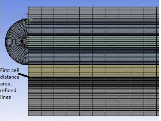
Figure 24 Mesh with refined boundary layers towards the wall ... 35
Figure 25 Snapshot of the right side of the pyrometer model's Mesh ... 36
Figure 28 Turbulence specification method for water ...41
Figure 29 flue gas settings, linear interpolation ... 42
Figure 30 MATLAB Results ... 44
Figure 31 Sum of the flue gas radiation over the length of the pyrometer ... 44
Figure 32 Local flue gas pipe energy ... 44
Figure 33 Flue gas flow temperature ... 45
Figure 34 Water temperature... 45
Figure 35 Flue gas flow velocity ... 46
Figure 36 Water flow velocity ... 47
Figure 37 Result of a flue gas inlet temperature of 400°C ... 48
Figure 38 Result of a flue gas inlet temperature of 750°C ... 48
Figure 39 Result of a flue gas inlet temperature of 860°C ... 49
Figure 40 Result of a flue gas inlet temperature of 1100°C ... 49
Figure 41 Result of changing the cooling water inlet temperature to 5°C ... 50
Figure 42 Result of changing the cooling water inlet temperature to 15°C ... 50
Figure 43 ANSYS Temperature results ... 51
Figure 44 ANSYS Fluent calculated properties ... 52
Figure 45 Mass flows ... 53
Figure 46 Flue gas flow temperature ... 53
Figure 47 Water temperature ... 54
Figure 48 Cut section graph, mid-point at x-coordinate 1, 25 meters ... 55
Figure 49 Cut section graphs at the end of the pyrometer ... 56
Figure 50 Simulation Y-plus value ... 57
Figure 51 Result when adjusting the inlet flue gas temperature in ANSYS Fluent to 400°C .. 58
Figure 52 Result when adjusting the inlet flue gas temperature in ANSYS Fluent to 750°C .. 58
Figure 53 Result when adjusting the inlet flue gas temperature in ANSYS Fluent to 860°C .. 59
Figure 54 Result when adjusting the inlet flue gas temperature in ANSYS Fluent to 1100°C 59 Figure 55 Resulting values when adjusting the cooling water temperature in ANSYS Fluent to 5°C ... 59
Figure 56 Resulting values when adjusting the cooling water temperature in ANSYS Fluent 60 Figure 57 MATLAB Temperature results ...61
Figure 58 ANSYS Fluent temperature results ...61
Figure 59 Resulting properties used for linear interpolation in ANSYS Fluent ... 62
Figure 60 Properties calculated in MATLAB ... 63
Figure 61 Water outlet velocity profile ...16
Figure 62 Flue gas outlet velocity profile ...16
Figure 63 y-plus value above 5 of the flue gas pipe ... 17
Figure 64 y-plus value below 5 of the flue gas pipe ... 18
Figure 65 Corresponding results to the increased y-plus value ... 18
Figure 66 Temperature result with increased turbulent Prandtl number ...19
Figure 67 Temperature result with faulty heat conductivity ...19
Figure 72 Sketching and modeling tab ... 20
Figure 73 Dimensions in the geometry step ... 20
Figure 76 Sketch creation ... 22
Figure 77 Drawing a geometry ... 22
Figure 78 Location of the "Generate" button ... 23
Figure 79 Add frozen ... 24
Figure 80 Boolean operation ... 25
Figure 81 Creation of the water bend ... 26
Figure 82 Wall sketch ... 27
Figure 83 Water bend sketch ... 28
Figure 84 Water flow sketch ... 28
Figure 85 Water bend solid ... 28
Figure 86 Fluid surface ... 29
Figure 87 Solid surface ... 29
Figure 88 Mesh method ... 30
Figure 89 Edge sizing creation ... 31
Figure 90 Bias factor and type toolbox ... 32
Figure 91 Bias type ... 32
Figure 92 Water boundary layers ... 33
Figure 93 Water bend boundary layers ... 33
Figure 94 Boundary layer for the pipes... 34
Figure 95 Named selections ... 35
Figure 96 Creating named selection ... 36
Figure 97 Designating the named selections ... 36
Figure 98 Edge named selection ... 37
Figure 99 Surface selection (flow)... 37
Figure 100 Surface selection (pipe) ... 37
Figure 101 Solver setup launch window ... 38
Figure 102 Inside the solver part of ANSYS project... 39
Figure 103 Chosen turbulence model ... 40
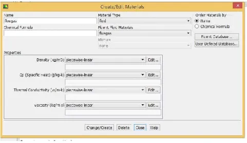
Figure 104 Materials ...41
Figure 105 Flue gas properties ... 42
Figure 106 Edit of interpolation table ... 42
Figure 107 Assigning all fluids and solids to their correct material... 43
Figure 108 Boundary condition of the water inlet ... 44
Figure 109 Inlet temperature specification for water ... 45
Figure 110 Outlet condition ... 45
Figure 111 Wall boundary condition... 46
Figure 112 Outer pipe external settings... 46
Figure 113 Symmetry axis settings ... 47
Figure 114 Solution methods settings ... 48
Figure 115 Solution initialization ... 48
Figure 116 Run calculation ... 49
Figure 117 List of result options ... 49
Figure 118 How to plot a list of results ... 50
Figure 121 Line point options ... 52
Figure 122 Temperature results from having 2500 steps, with Δx = 0,001 ... 53
Figure 123 Temperature results from having 25000 steps, with Δx = 0, 0001 ... 53
Figure 124 Temperature result from having an inlet velocity of 1, 5 m/s ... 54
Figure 125 Pressure from having an water inlet velocity of 1,5 m/s ... 54
Figure 126 Temperature from having an inlet water velocity of 2m/s ... 54
Figure 127 Pressure from having a water inlet velocity of 2m/s ... 54
NOMENCLATURE
Designation Description Unit
Thermal resistance °C or Kelvin /meter
Fluid temperature in fluid x °C/Kelvin
Temperature at point x °C/Kelvin
Overall heat transfer coefficient at point x
, μ Dynamic viscosity of fluid x
Kinematic viscosity of fluid x
Prandtl’s number of fluid x [-]
Heat conductivity of fluid x
,
Nusselt’s number based on diameter [-]
Convection coefficient of fluid x
,
Local energy inside one pipe W
Energy based on the overall heat transfer coefficient
W
Reynold’s number based on diameter [-]
Specific heat of fluid x
, Mass flow of fluid x
Diameter of pipe x Meter
Designation Description Unit
Single pressure loss [-]
Pipe friction [-]
Density of fluid x
Velocity of fluid x ⁄
Length of section x Meter
Radius of section x Meter
Hydraulic diameter at point x Meter
ABBREVIATIONS
Förkortning Beskrivning2
INTRODUCTION
First part of the thesis will contain a brief introduction of the studied object (pyrometer, thermocouple) and few selected aspects regarding suction pyrometer.
2.1
Background
Emission out of a global aspect is a much-known issue in today’s society, more specifically CO2 known as carbon dioxide that is a next-to unavoidable emission from combustion systems. This is due to the reason that most substances and fuels utilized in combustion contain carbon that reacts with the tertiary air in boilers. However, other less known emissions exist that engineers constantly work with to reduce in combustion systems that can have a significant impact on both efficiency and human health. This can be understood as well by looking at the combustion triangle that say that a successful combustion requires fuel, heat and air.(Fuchs, 2012)
One method of optimizing the carbon dioxide emission rate from combustion systems is the systematic use of industrial combustion testing of boilers, which is a method of gaining knowledge of a boiler’s combustion phenomena (emission formation, etc.) and performance (efficiency). Accomplished by measuring temperature and gas composition in different positions of the boiler that can help to improve efficiency and hence reduce CO2 emissions (Konstantinos, 2017)
It can as well help to reduce or better control other emissions as nitrogen oxides that goes under the collection name of NOx and carbon monoxide (CO). These two emissions are heavily temperature dependent. For example, NOx is created from temperatures in the combustion chamber being excessively high that can cause damages and reduction of efficiency, CO is created when temperatures are instead too low that correlates with incomplete combustion, one cause can be the lack of air supply when again looking at the combustion triangle. Worth mentioning is also dioxins that is created from waste incineration of plastics which is highly toxic substance, meaning proper equipment has to be in place when utilizing waste incineration.(Cleaver-Brooks.com, 2016, p.; Konstantinos, 2017)
Determining the concentration distribution of the flue gases will give a deeper insight into the boilers combustion phenomena and therefore give a better understanding of the emission/pollution formation mechanisms. A good understanding the boilers air supply can be crucial information in the sense that it can avoid disastrous malfunctions and or creation of CO from the lack of proper air supply.(Cleaver-Brooks.com, 2016) The flue gases composition is determined by accompanying equipment that has the possibility of analyzing such content.
These improvements and measurements of temperature distribution and gas composition of a boiler is achieved by utilizing a suction pyrometer.
Experimental work is an important part of combustion research and the process of building mathematical models. The most important and critical parameter is temperature along with its distribution in experimental work as it can be correlated, directly and indirectly, to heat transfer, emission formation, corrosion etc. Making temperature and its distribution very valuable. In heat transfer theory, temperature is the key parameter for consideration as this variable can be used to directly explain how heat will travel through an object.(Incropera et al., 2005; Konstantinos, 2017)
Several conventions, policies and laws are in place that has the purpose of mitigating the amount of carbon dioxide emissions into the atmosphere. Article 2 of UN’s framework convention of climate change has the ultimate objective of stabilizing greenhouse gas concentrations to such a level that will prevent anthropogenic interference on the climate system. As well, ensure food production and enable economic development. (United Nations, 1992) Noticing that these goals are part of the sustainable energy definition. In UN’s document, “Our common future” say that the humanity has the ability to develop a sustainable energy system in such a length that it will meet present demands as well as future generations. (United Nations, 1987)
The most recent mitigation policy is the Paris agreement that 195 countries signed. It is the first-ever global agreement that is legally binding. One of the key points of this agreement is the goal of avoiding an increase of global temperature above 2°C.(Paris Agreement, 2016) The 2°C is a much-known project that has been in play since 2009 agreed upon in the Copenhagen climate conference.(Knutti et al., 2016) Although this agreement goal, carbon dioxide from combustion and cement systems have continued to grow by approximately 2, 5 % per year. (Friedlingstein et al., 2014)
2.1.1
Previous research
Previous research on the specific point of pyrometer cooling is very vague and lacking sufficient information to use as a comparison in this study’s work, therefore there will be lacking reference for this purpose and the study will be validated through the use of two different simulation platforms, MATLAB and ANSYS Fluent. The most popular research is the temperature accuracy of the thermocouple.
Around this subject of study the most significant differences are of thermocouple sizes and type. One or more radiation shields where the emissivity differs due to different material and temperature regions. The sheath surrounding the thermocouple and shield can be made of different materials as steel or ceramic. With the requirement to be able to withstand up to 1000°C (waste incinerator for example) (Loyd, 2013)
The study of bare and aspirated thermocouples in compartment fires evaluate the thermocouples temperature accuracy by creating an analytical model of single/double shielded thermocouple. By varying flue gas suction velocity and surrounding temperature.
The surrounding temperature vary illustrates different measurement positions. (Blevins and Pitts, 1999)
Another study is the “Estimation of radiation losses from sheathed thermocouples” that essentially evaluate a similar temperature measurement accuracy as the first stated paper. Difference being sheathed vs un-sheathed pyrometer tip.(Roberts et al., 2011)
What both of these studies have in common is the focus of accuracy of the thermocouple by using analytical models and carrying out physical tests.
The gap of research is regarding the significant difference in research focus. Temperature accuracy vs. sufficient water cooling. As already stated the focus of this study is the water cooling of a newly designed suction pyrometer by Jan Skvaril, PhD at Mälardalens University
2.2
Problem formulation
This thesis will handle the performance testing of a pyrometer, of its water cooling by heat and mass transfer methods with the critical parameter being temperature as with this variable it is possible to explain how the entire performance and temperature distribution will be.
Meaning that the performance testing will consist of creating thermal resistance networks for the pyrometer body. It is designed in such a way that the pyrometer body consist of three pipes within each other with the innermost pipe containing the flue gases to be cooled (See figure 6). The MATLAB calculations is compared with a CFD simulation program called ANSYS Fluent, which a 2d-Axisymmetric model is constructed in.
2.3
Research question
What demands needs to be met in order to keep the tool from getting damaged by high temperatures and to maintain a steady operation and cooling?
2.4
Delimitation
The thesis will only focus on the suction pyrometer itself and its corresponding calculations performed on it. Due to the nature of the heat and mass transfer methods, it will go under the assumption that the reader has engineering level knowledge of these types of calculations. As well as knowledge of what the variables purpose are such as emissivity. Understanding what temperature/velocity profile is.
Pyrometers and its use regarding industrial combustion testing is explained in such a way that the reader will understand the importance of utilizing this tool and what knowledge it will bring by its use
Programs used for calculations and comparison will not either be explained in detail except sufficiently enough that the reader understand which are used for what purpose and for which reason. And sufficiently enough to be able to follow and replicate the results.
2.5
Aim and scope
To determine the temperature distribution of the pyrometer’s water cooling system and out-going temperature of the flue gas. Conduct a literature study containing information
regarding the subject of pyrometers and its connecting usage possibilities. Parallel to these calculations information of the pyrometer’s water flows, pressure losses are determined to observe that the cooling is being carried out with sufficient pressure.
3
INTRODUCTION TO PYROMETERS
A pyrometer is essentially a thermometer, very much relatable to those existing in most households today. It works by the same principle except that a pyrometer is designed for high temperature areas, such as apartment fires, industrial boilers and other high temperature areas that are of interest to measure with this type of tool.
Pyrometer is a word originating from the Greek words pyro meaning fire and meter meaning to measure. The first pyrometer that was used was invented by the potter Josiah Wedgwood in 1783 (BBC.CO.UK, 2014) for temperature measurement in his kilns, although it has been questioned if he was the true inventor of this tool.(EduBilla.com, 2017) It was achieved by comparing the sizes of clay being heated to different known temperatures as the clay would shrink depending on temperature.
3.1
Examples of pyrometer types
First modern pyrometer became available 1901 when L. Holburn and F.Kurlbaum built the first disappearing filament pyrometer. It operated by using a thin heated filament above the object to be measured and when the filament disappears the temperature was then read from a scale located on the pyrometer. Although this type of pyrometer turned out to have its faults due to being heavily dependent of objects emissivity which is highly temperature dependent and other aspects of the object such as surface roughness. Meaning extensive knowledge of the emissivity was required. This is a manual measurement type, as the temperature
measurement is conducted by observing with the human eye on a scale that was located on the pyrometer tool. This is also known as an optical pyrometer. (EduBilla.com, 2017) Overall it can be divided into two main types. Optical and digital with the main difference being as stated manual measurement vs automatic.
Without going into a larger amount of detail of different types of pyrometers but most common today is to use digital measuring devices which can as well be divided into two subsections. (Woodford, 2016)
An example of an absorbing light pyrometer is the infrared (IR) pyrometer. It is a sensor that measure radiation from the target objective as all bodies above zero Kelvin will emit an infrared light proportional to the body. It works by the principles of radiation laws. Although solid bodies usually do not have any infrared transmission. This due to Kirchhoff’s law it is assumed that the radiation is absorbed by the body and therefore increasing its temperature hence increasing amount emitted. A simplified explanation is that the IR-pyrometer
measures the temperature by photographing heat radiation, by this fact the accuracy works very much the same way as a normal camera, the lens will determine which wavelengths of radiation that can be intercepted. The lens is important to pay attention to because of the wavelengths, an example is that a wavelength of approx. 2 µm operate at a temperature of 600°C meaning the pyrometer would stop measuring if it would be below the stated
temperature.(Gruner, 2003)The lens has the job of focusing the thermal radiation from the target object to the receiver (detector) that converts the radiation into an electric signal. (Electrotechnik.net, 2017)The wavelength is corresponding to the temperature, as
temperature increases of an object the wavelength increase.(Electrotechnik.net, 2017)The largest difference compared with the suction pyrometer is the fact that IR-pyrometer measures the targets temperature compared to a mean temperature.(Pentronic.se, 2017) Another example is the optical pyrometer which is as stated regarding the disappearing filament pyrometer, what the optical does is a brightness comparison to measure the objects temperature. This is done by using a light bulb that can be adjusted to match the brightness of the object to receive a reference temperature as the light intensity is proportional to the temperature.
The heat radiation is emitting from the object and captured by the contact lens which has the purpose of focusing the thermal radiation to the reference bulb. This is where the
disappearing filament is used. If the reference bulb is dark, that means having a temperature cooler, if brighter the temperature is hotter. When the filament disappears the reference temperature has reached equilibrium with the objects temperature.
After final adjustments are made, the current is measured with a voltmeter which is proportional to the temperature. (John, 2011)
Heat absorption type of pyrometer is the suction pyrometer as an example. That do
temperature measurement by having gas flow over a thermocouple at high velocities. It can be designed with a sheath or non-sheathed, one-radiation shield or more. The shield or more properly called radiation shield has the purpose of negating the negative effects of radiation while the sheath protects the thermocouple from high temperatures of the test area.
The thermocouple is measuring the temperature by converting heat directly into electricity, it comes in several different types that is mostly decided by required temperature range and cost. The direct conversion of heat into electricity is called the Seebeck-effect. After which an interpolation table can be used to calculate a corresponding temperature to the induced voltage. (thermocoupleinfo.com, 2017)
Generally a suction pyrometer is a long water cooled device. It can either be circular or rectangular cross section. The length varies from design to design, of this study the pyrometer is 2, 5 meters long but up to 6 meters in length exists. The front of the tool is covered by a sheath that can be made of either steel or ceramic, in most cases the tool is surrounded by a radiation shield as stated above.(Loyd, 2013) In the other end is the connection point that is connected to a voltmeter which is indirectly the temperature measurement. The body of the tool consist of several pipes, depending on design, with essentially in all designs having water circulating around the hot flue gas pipe.
In this design the flue gases flow within the innermost pipe, the cooling water pipe with ingoing flow is surrounding hot the flue gas pipe. The outermost pipe is for outgoing water flow.
Overall the design of a suction pyrometer is quite simple. The most advanced point is the tip as the temperature accuracy can be improved depending on design and material used.
3.2.1
Seebeck effect and thermocouple design
The physicist Thomas Seebeck (1770-1831) originally found the Seebeck effect by observing a compass, the needle would be deflected when he created a closed circuit between two
different metals at different temperatures and originally determined this to be cause of induced magnetism, possibly Earth’s magnetic field. But was later realized to be due to Ampere’s law by which a thermoelectric force would deflect the needle by inducing an
electrical current. Summarized is that the temperature difference of a closed circuit can drive a voltage, this became known as the Seebeck effect. (CalTech, 2017)
The Seebeck effect plays its part in the design of a thermocouple. A thermocouple consist of two different metals that are joined together at both ends. When heated in one end it will create a continuous flow of current. This junction can have several different setups which are grounded, ungrounded or exposed. (Omega.com, 2017; thermocoupleinfo.com, 2017)
Main difference being that in a grounded, the thermocouple wires are attached to the probe walls resulting in a good heat transfer through walls to the junction by conduction.
response time but give electrical isolation. Exposed is mainly what it sounds like it is a thermocouple bead that has no sheath or radiation shield.
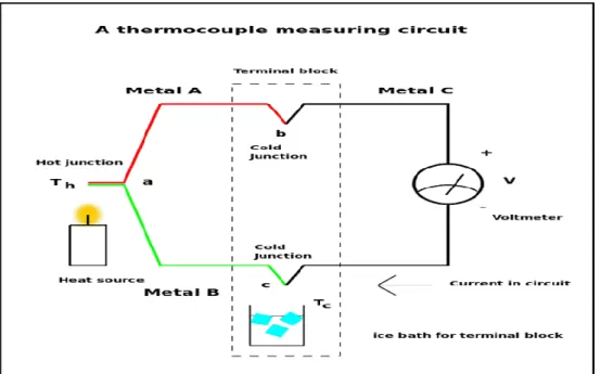
Figure 1 Thermocouple measuring circuit with a heat source, cold junction and voltmeter (Wtshymanski, 2011)
The thermocouple is as stated much like a thermometer, it only measures its own
temperature which in a suction probe due to thermal radiation, convection and to a small part conduction be a mean temperature between the true gas temperature and the
thermocouple tip. The above figure is a sketch of how the thermocouple measure temperature. (Loyd, 2013)
3.3
Water cooling
The stated temperature measurement methods are explaining the “tip” of the suction pyrometer. Cooling is crucial due to the flue gas can have temperatures as high as 1000°C (waste incinerator as an example), this is dependent on measurement position inside the boiler, close to or far from the fire bed. A few important factors include having sufficient flow to avoid evaporation of the water, and damages as the pyrometer could be overheated and the metal could start to bend inside test area. Conditions such as amount of flow and inlet
temperature will determine the amount of cooling that can be achieved.(Loyd, 2013)
3.4
General calculation and validation method for this type of tool
The most efficient way of explaining the performance of a suction pyrometer is the use of heat and mass transfer correlations. Type of equations and balances vary depending on the aim of calculation. If the aim is the measurement accuracy of the thermocouple it will be a
focus of energy balances that include radiation and convection as the major parts of the thermocouple.
The water cooling and heat transfer of the pipes is mostly efficient explaining using thermal resistance networks. This means calculating overall thermal coefficients known as U values that is dependent on convection and conduction for the major part and no attention to the thermocouple is required as its temperature will follow that of the flue gases.
In temperature measure accuracy calculation the most efficient way of validating the analytical model is to do physical measurements in order to efficiently see how it will compare which is the popular way of testing the models according to a number of studies in this area, See previous research.
3.4.1
ANSYS Fluent
ANSYS CFD Fluent is a simulation program for solving heat and mass transfer problems. A model is created using a part of the program that is much like using a CAD program, meaning the first step is always to draw the object to be simulated and in the same step define the diameters of the model.
Next step which is the most time consuming is adding mesh. The mesh is the point of where the object is affected by the different types of heat transfer.(ANSYS Fluent, 2017.)
3.4.2
MATLAB
MATLAB is chosen due to its flexibility in programming all the required correlations and due to the need of multiple loops for iteration of the temperature distribution. The thesis will contain a significant amount of these types of calculations.
MATLAB is a universal programming program using its own type of language. It contains optimal tools for plotting temperature distribution graphs, among other options.
The pyrometer is divided in several sections in MATLAB due to thermal resistances. The fluid temperatures are affected by each other, meaning the construction of the code will occur in steps. By following the structure of building within and moving the required loops outward.
4
METHODOLOGY
The objective of this study is straightforward, therefore a detailed methodology of the
analytical model is presented in such a way that the reader will be able to follow and replicate the results obtained. All coding of the analytical model is conducted within MATLAB while
the validation of MATLAB results are obtained by utilizing the simulation program ANSYS Fluent CFD of where a simplified axisymmetric 2D-model is created.
All the presented figures contained in method, result, description of study and the appendix is created by the author is this thesis for the sole purpose of use in this thesis.
4.1
Literature study
The literature study is conducted by searching for valid information regarding heat transfer by thermal resistance networks that are mainly explaining the methods behind these options. As well as literature of previous courses are used to obtain certain data and/or effective equations with the purpose of calculating a property.
Due to the nature of going the other direction of calculating the cooling of the pyrometer, the information is a lot scarcer then temperature accuracy studies that can be found.
4.2
Calculation pathway
It will start explaining how it is solved with the help of MATLAB by using stepping calculations with balances based on calculations cells or nodes.
Initial figures will explain how node dependence is created. The next figures illustrate the design which has been simplified from the original design of the suction pyrometer.
Before moving further, due to the thesis will handle pipes. The presented coordinates will be of cylindrical form. Meaning the x-axis is explained as “z” which is the length, while the y-axis is “r” which is the radius.
4.2.1
MATLAB
As previously mentioned the code is executed using a stepping length that can be set before running the code.
Defined as / where is the adjustable stepping size. This allows for setting the desired number of steps between each temperature calculation the model should take, which is also the length the FOR loop will step. Meaning the FOR loop will conduct the same amount of iterations as the number of nodes making it a direct correlation to the length. The length inserted, is the length of the pyrometer pipes (2, 5 meters) which is the same for the flue gas pipe and water pipes.
Figure 2 illustration of a calculation cell
This figure illustrate how one calculation cell is setup, which can be used to explain the reason of the balances are setup as they are which is due to the importance of keeping the balance within the calculation cell.
Figure 3 Illustration of nodes
This figure illustrate how the nodes or calculations cells are considered when creating the MATLAB code. N-1 of figure 3 can be seen as the “inlet” value while n is seen as the outlet value. This is important to keep in mind when setting up calculations. If wanting to move even further back or forward, it can be done by increasing the number n-2, n-3 if going backwards of n+2, n+3 if going forward etc.
MATLAB is a sub-sequential solver making it important to keep in mind which variables is written into the script first, a sub-sequential solver means that the solver will go from the top down, meaning it will execute the code in steps, For instance, the assumed temperature needs to be defined before adding temperature dependent correlations, this way the code will understand that it has an input variable.
Due to the extensive possibilities that exist in MATLAB of what it can accomplish as it is a universal coding program, meaning it is not strictly limited to the use of heat and mass transfer problems. It will therefore not be explained more than briefly. What will be
explained is the different utilized features available in MATLAB and how and why they were chosen for their task as the previously explained calculation steps is the same that is taken in MATLAB.
In the code the temperatures is defined as T_mw = t_w1(n-1); Which mean that the
properties will be calculated of the actual step depending on the temperature of the previous node as an inlet value.
Syntax is the designated name of code MATLAB use to execute certain features, will use this word when explaining what kind of features that is utilized for the study.
What will be the major change from using the equations in their basic form is the use of mentioned calculation cells or nodes.
= ( / ) + Eq 3.
If taking this formula in its basic form and converting into MATLAB syntax and node
dependence it will have the form of (see the (n) parts of the equation, which mean that n will change number of each iteration when moving forward until reaching the end value, which is determined by Δx)
= ( ( ) ( )/ ) + ( ) Eq 3.
Or t_w2(n) = ((qUA2(n) - qUA3(n))/(m_w*1000*Cpw_tw2(n))) + t_w2(n-1);
The above equation illustrate the MATLAB syntax and is applied throughout the entire study.
= / , .
( )= /
Meaning the inlet temperature for the equation will be n-1 while the outlet is n, if seeing out of an energy balance stand point.
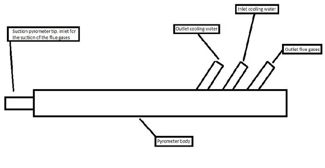
Figure 4 Side view of the suction pyrometer in a simplified form
Overview of the suction pyrometer from its side. With indicatory text illustrating the inlets and outlets. Although the calculations are performed according to figure 6.
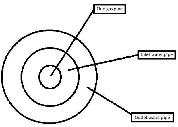
Figure 5 Front view of the suction pyrometer
This view is if rotating the pyrometer so the tip is pointing towards the reader, see figure 4 for the location of the tip. The figure illustrates how the pipes are positioned inside the pyrometer body.
4.3
Heat transfer correlations and balances
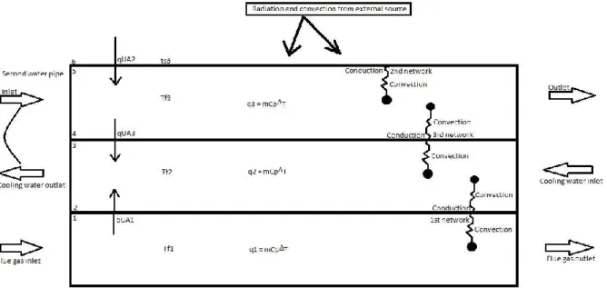
Figure 6 Overview of how the pipes and energies are setup. Illustrating how the balances are derived The water outlet temperature (Designated as “Cooling water outlet”, see figure 6) is unknown and an assumption, an iterative process is required to reach the desired known cooling water inlet temperature. This temperature is then set as equal (see the line in the left side of figure 6)
An iterative process is the process of repeating calculations or analysis to arrive at a desired state or result. The goal is by each cycle of calculation reach a result that is closer to the desired result until finally reaching a final result.
As in the case of the iterative process of reaching the desired inlet temperature of 10°C, in terms of this process, it is the continuous guess of the outlet temperature until the equation match the set term of the desired inlet temperature
Again keeping in mind that the calculations are done in steps, this figure can be considered to be divided into 250 cells in the z-direction if using a Δx of 0, 01 meters.
It is assumed that the energies of each pipe is symmetrical, therefore the pyrometer could be cut in half, much like stacking the pipes on-top of each other and divided into three sections designated as q1, flue gas. q2, inlet water pipe. q3, outlet water pipe as figure 6 illustrates. The arrows are indicating inlets respectively outlets of the fluids, while the overall thermal energies (qUA) arrows are indicating in which direction the heat is travelling between (through) the pipes and from these arrows it can be understood which pipe is being heated respectively cooled which will be realized further into the explanation when the balances are
4.3.1
Diameter and radius
With the suction pyrometer consisting of three pipes as mentioned, this will result in the use of three inner diameters with three corresponding outer diameters.
Figure 7 Inner and outer diameter of all pipes with their MATLAB designations
Outer diameter is defined as = + (2 ) this is valid for all the pipes.
The radius which is necessary for the thermal resistance network is obtained by = , x will change depending on the affected pipe.
In the case of calculating the Reynold number for the water pipes, the hydraulic diameter is necessary. Defined as = where the subscripts 2 and 1 indicate larger diameter respectively smaller diameter of the pipes. Source :(Incropera et al., 2005), page 519-520
4.3.2
Thermal resistance network
This subsection will explain how the thermal resistance network is applied to the analytical model and the reason behind why they have the form that is presented.
Figure 6 is illustrating how the thermal networks are drawn and which effects that are included. Figure 4 show the location of these networks.
Figure 8 Thermal resistance network illustration
Due to being constructed of pipes, the thermal resistance network will be of radial coordinates that has the form of:
=
1
=
ln (
)
2
Equation source: (Incropera et al., 2005) Figure 7 highlights how the radiuses are used in the conduction resistance. The same principle is applied for the other pipes with the mid-point of the flue gas pipe as base of origin as these will change depending on the position of the network.
Figure 9 illustrating the radiuses used in the conduction formula
The thermal resistance networks designated as 1st and 3rd (see figure 4) have the form of Eq .1
, 1 =
1
+
log ( 2 1)
2
+
1
,
1
The difference being switching out flue gas convection coefficient for the convection coefficient for water at the second water pipe, first term on the right side.
, 3 =
1
,+
log ( 2 1)
2
+
1
,3
Source : (Incropera et al., 2005)
Where the areas are calculated with
.
=
This formula calculates the area per stepping length, meaning the area of one node or “calculation cell” of the convection resistances.Depends on where the heat transfer is occurring for that network, and if inner or outer diameter. This area calculation is valid for all thermal networks presented in this study. The conduction thermal resistance is as well calculated per calculation cell by multiplying with as it is a correlation for the length for one calculation cell.
The last network that is acting towards the pyrometer surface (ts6) is a combination of an energy balance and using overall heat transfer coefficient that have the form = 2 ( ) Designated as the 2nd network. This network is used to obtain the external impact
from free convection and radiation. By observing Eq. 1 and Eq. 3 it can be seen the similarities it share with Eq. 2 with the difference of one less convection term which is replaced by the overall thermal energy.
, 2 =
1
,
+
log ( 2 1)
2
2
To avoid the complexity of view factors the radiation is assumed to affect a small object in a larger surrounding, therefore validating the use of
=
(
)
Free convection from flue gases inside the boiler or area of measurement will as well affect the pyrometer surface and is of the standard form for convection
=
(
) Source :(Incropera et al., 2005), page 9
Meaning the energy balance will be
=
+
for which is used to solve for ts6.Having thermal resistance correlations complete. The overall heat transfer coefficient is calculated by = 1 where is the total thermal resistance for that specific
Notable about the thermal resistances are their similarities to other coordinates. For convection the formula has an identical form as for the plane wall.
= 1
While for conduction it changes from radius dependence to length, i.e. for one-dimensional conduction of a plane wall, the temperature will be a function of the x- coordinate. Meaning heat is transferred solely in this direction, has the form of = . Reason behind this explanation is due to these conduction formulas will have similar results and can therefore be used as a comparison.
Source: (Incropera et al., 2005) , page 96
4.3.3
Heat balances
Heat balances is this study is the most important part as it is with the help of these that makes it possible to calculate the temperature distribution of the suction pyrometer. Heat balances for the individual pipes are obtained as follows with the basic energy balance of = . Has the form for each pipe as follows. Source :(Incropera et al., 2005), page 17
( ) = ( )
( ) = , ( )
( ) = , ( )
In MATLAB these are calculated as ( ) = ( ) ( ) meaning the energy is calculated for each step, these equations are later summarized with the function “sum”
q1(n) = m_g * (Cpm_t12(n)*1000) * (t_g2(n-1) - t_g2(n)); q1_sum = sum(q1);
q1(n) is the MATLAB code for calculating the energy per stepping length.
Sum(q1) summarized the q1 vector into a single value, allowing to observe the total energy contained of that pipe. The process of obtaining the other summaries are identical as the presented ones. Note how the (n-1) and (n) are used from seeing figure 3.
Notable is the difference from switching versus of the flue gas and water balances. This is due to the water is being heated while the flue gases are being cooled. 1 and 2 designate the different pipes.
By observing figure 6 it is realized of how the pipes will affect each other from which the energies of these can be obtained by utilizing thermal resistance network.
Using these balances allows to calculate the temperatures of the fluids without requiring knowledge of their respective surface temperatures of the pipes, the balances will have the form as they have with the thought process of realizing which fluid will be warmer for that balance for which the equations can be created. At this point it can be observed how the overall heat transfer coefficients are utilized. Thought process of the temperature differences used is warmer minus cooler.
( ) = ( )
( ) = 2 ( )
( ) = 3 ( )
The effects are designated 1-3 in relation to their respective thermal networks.
These effects are summarized in the same way as previously stated. The overall heat transfer coefficient and area are values that will be changing for each step, but in the code not put into a vector as it will still serve its purpose and have the ability to sum up the energies.
The important relation these balances bear to each other is how they can be connected to each other by combining the energies as the ones stated below
=
= +
=
By observing figure 6 the final temperature calculations formulas can be set. The parentheses indicate which fluid temperature these derived equations calculate.
( ( )) = ( ) ( / ( )) Eq 1.
MATLAB syntax: t_g2(n) = t_g2(n-1) - (qUA(n))/(Cpm_t12(n)*1000*m_g));
Eq 1. After combining the heat balances and solving for an explicit outlet flue gas temperature. Designated as first fluid temperature. The same principle of solving for an explicit temperature is applied for Eq 2 and Eq 3
( ( )) = ( ) ( + / , ( )) Eq 2.
MATLAB syntax: t_w1(n)=t_w1(n-1)-((qUA(n)+qUA3(n))/(Cpw_tw1(n)*1000*m_w));
Eq 2. The actual temperature of interest is the calculation of the outlet water temperature, but in this case the inlet temperature is calculated due to the outlet temperature is unknown and is instead a guessed value to reach the desired inlet temperature of cold water.
Designated as second fluid temperature
MATLAB syntax: t_w2(n)=((qUA2(n)-qUA3(n))/(m_w*1000*Cpw_tw2(n)))+t_w2(n-1);
Eq 3. Is the third and final fluid temperature leaving the suction pyrometer. At this stage, the inlet temperature of this pipe is known which the outlet temperature of the first water pipe. (See figure 4)
The specific heat of water is separated in two vectors the water temperature is separated in two vectors for which the properties are calculated separately for each water temperature vector.
The last heat balance is the overall balance that controls that the effect of the flue gases match that of the water.
=
,(
,+
)
=
, ,Overall energy balance can be easier understood with previously used designations, these can be written in two ways.
= (
) +
(
) +
(
)
=
+
(
) +
(
)
The total energy the water is experiencing can be written in two ways as well by observing the previously stated combinations that can be done between the energies. Although the latter is used in MATLAB.
=
+
= ( (
) + (
) )
(
)
(
) )
The overall energy balance is a requirement that the amount of heating the water is
experiencing has to be equal to the amount of cooling the flue gases experience, this includes the external impact of radiation and free convection
=
= 0
Source : (Incropera et al., 2005) , page 13
The explained heat balances are the correlations required for a complete temperature distribution.
After doing a cycle of calculations, the effects are now known at this point meaning that the surface temperatures can be calculated. This is done by using the convection coefficient termed as = where = . It has this form due to the fluid is transferring heat to the surface. The balances use the same principle as for the effects derived from the overall heat transfer coefficient. Source : (Incropera et al., 2005), page 9
Therefore, the balances for the surface temperatures will have the following forms, see figure 4 for the number designations of each surface
= = ( ) = 1
= When solving for surface temperature of the flue gas pipe.
The surface temperature equation will have the same form for all of the surface temperatures due to having the same form of = . What will differ is the diameter (Area)
4.3.4
Water and flue gas properties
With heat balances and thermal resistance networks complete. The calculation of various properties are required for temperature distribution calculations to begin.
As the key parameter is temperature, the majority of the properties can be calculated using temperature based interpolation formulas. Those properties who are not calculated using a formula will be calculated using linear interpolation with data that is being directly imported into MATLAB.
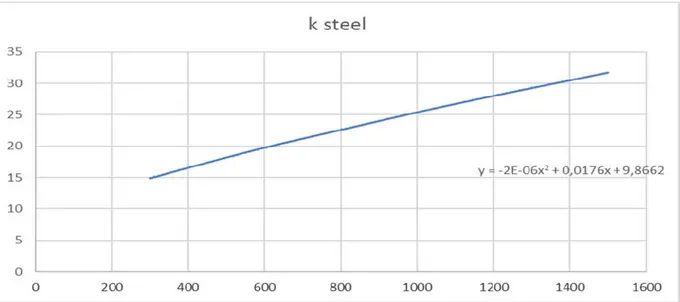
The interpolation formula is created by using the trend curve feature available in Microsoft Excel. Due to the amount of interpolation formulas used for this study, the tables used for their creation are presented in the appendix.
List of required properties for initial calculations to begin that use an interpolation formula
1. Specific heat for flue gas and water, Designation
2. Dynamic viscosity for flue gas and water, used for the calculation of Prandtl number and heat conductivity, Designation μ
3. Kinematic viscosity, used for the calculation of Reynold number, Designation
4. Density for flue gas and water, used for the calculation of velocity, mass flow and pressure loss calculations, Designation
5. Heat conductivity for steel and water, used for the calculation of convection coefficient and thermal resistance for conduction, Designation
Figure 10 Screenshot from Microsoft Excel illustrating the trend curve for heat conductivity of AISI 304 steel. Y-axis is the heat conductivity values with x-axis ranging from 300 – 1500 Kelvin
The exact same principle is used for all the created interpolation formulas, figure 9 illustrate the equation for steel. The type of equation chosen is polynomial as it can be fitted to the curves with the least margin of error.
4.3.4.1.
Created interpolation formulas
Specific heat for flue gases is derived from an assumption that there is a certain amount of air, therefore performing a linear interpolation for the mean value of flue gas specific heat. Meaning the specific heat is calculated using two polynomials for air respectively flue gas. The temperature of the equations for flue gas and water are both based on Kelvin
The mean specific heat is then defined as = + ( )
Both polynomials of air and flue gas use the same form = 1000
1000+ 2 1000 + 3 1000 + 4 1000 + 5 1000
(
1000+ 2 1000 + 3 1000 + 4 1000 + 5 1000 ]
and designate actual and previous temperatures respectively. Source : (Wester, 2012)
Specific heat for water is based on a pre-created excel sheet, based on four constant values defined as
= 2,1103 10 = 5,3469 10
, = + , + , + , ,
To obtain the specific heat in kJ/kg, K, , is divided by 18 Reason behind dividing by 18 is because water has a mass of 18 Source : (convertunits.com, 2017)
,
18 = ,
Source : (A.K Coker, 2017)
Dynamic viscosity formula for water are created from tables, and is dependent on the fluid temperature of water. The temperature is in °C
μ = 9,67 10 8,207 10 , + 2,344 10 + , 2,244 10
,
Kinematic viscosity formulas depend on the fluid temperatures and are in °C
= 5 10 , + 3 10 , 7 10 , + 8
10 , 5 10 , + 2 10
For flue gases the kinematic and dynamic viscosity is calculated with linear interpolation directly in MATLAB based on a table of values. How this is conducted is presented in the MATLAB sub-section and the full code of the function file is observable in the appendix. Formula for the density of water is correlated from an excel sheet containing density data per degree Celsius
= 1000 (1 , + 288,9414
508929,2 , + 68,12963 ( , 3,9863)
Source : (Maidment et al., 1993)
Density for the flue gas is as well calculated with linear interpolation. Source of table : (Pipeflowcalculations.com, 2017)
The heat conductivity of water and steel. As the temperature of the material will follow that of water, the two formulas will use the same temperature.
For water
= 0,5752 + 6,397 10 , 8,151 10 ,
Table source: (Incropera et al., 2005) , The assumed material is AISI304 Steel.
4.3.5
Equations for properties
The presented equations are those used for calculated various properties when there is no need for an interpolation formula or linear interpolation.
The stated equations are calculated either using values from the interpolation formulas or by having an assumed value.
=
Heat conductivity, can be used for all materials and fluids. This equationdepends on the dynamic viscosity, specific heat and the Prandtl number. (EngineeringToolbox, 2017)
The same form of the equation can as well be used to calculate the Prandtl number for water as an interpolation formula is available for heat conductivity of water.
=
Prandtl numberFor calculation of the Nusselt numbers. Required for the convection coefficient, certain formulas can be used depending on the situation of free or forced convection, if it is laminar or turbulent flow.
This knowledge is gained with the calculation of the Reynold number
=
If Reynold number is less than 2300 it is considered laminar while above 5 10 it is considered fully developed turbulent flow. Between these two values is the transition range. Source : (Incropera et al., 2005) , page 487 & 515
Is the mean velocity, which varies over the cross section of the pipe
=
Source: (Incropera et al., 2005), page 487As the area is a part of the mass flow formula it will look slightly different for flue gas and water respectively. Which is due to how the pipes are located in regard to each other. For flue gas the mass flow formula is as presented.
For water it will be
=
(
, )This area differs from that of the one utilized in the thermal resistance networks. Here it requires the circumference area, defined as
=
because the flow affects the entire “circumference” of a pipe.The mass flow is initially calculated with a set velocity of water and flue gas before redoing the velocity calculations by making it dependent on the temperature via the density. The flow is assumed to be turbulent and fully developed.
The assumption of fully developed flow only regards internal flow and does not affect free convection. It has to do with the reason that flow require a certain length to be fully developed, this length is termed the hydrodynamic entry length. Due to the high velocities and short length of the suction pyrometer it is instead considered to be fully developed from the start. (Incropera et al., 2005), page 487
= 0,023
The exponential depends on if it is cooling or heating for which n = 0, 3 respectively 0, 4. For calculating the free convection of the external impact the Nusselt number is calculated with the following equation. This equation is valid over all ranges of Reynolds number and is defined for a cylinder in cross flow.
= 0,3 +
0,62
1 +
0,4
Pr
1 +
282,000
Source :(Incropera et al., 2005), page 427
The convection coefficient regardless of condition is defined for cylindrical systems as
=
making this a valid equation for the calculation of all convection coefficients. What makes the convection coefficients differ is the use of different Nusselt numbers due to having certain requirements depending on situation, heat conductivity coefficient will change as well depending on the material or fluid affected, and the diameter. The presented Nusselt numbers are only for cylindrical coordinates.4.3.6
Pressure loss calculations
The pressure loss calculations do not affect the temperature distribution calculations, will be presented as an indicatory value that the amount of water used for cooling is not exceeds the maximum allowed pressure of the pipes.
=
2 + 2
Where f is the friction coefficient = (0.790 1,64) . 3000 ≤ ≥ 5 10 is the single pressure loss of a bend, this bend is located at the point where the water is entering the second water pipe. This equation is called the Darcy-equation. Which is a correlation for the loss of head due to friction. (Bansal, 2005)
Source : (Wester, 2012)
4.3.7
Flue gas radiation
Radiation from the flue gases are calculated as a check to see if it will have a significant impact on the temperature of the flue gases as well as how large the radiation will be due to the high gas velocity at the suction pyrometer inlet.
The surface temperature of doing this calculation will then make it a necessity for which the used equation is presented on page 19 of study.
The flue gas radiation function is based on temperature and partial pressure dependent tables, these tables calculates the emissivity and absorptance of the gas. From these tables a model was created by Kristoffer Hermansson, M. Sc in Sustainable energy systems at Mälardalens University and used with permission in this study. (Hermansson, 2015)
From which calculates the flue gas radiation with temperature, pipe diameter and the surface temperature of the flue gas pipe as input variables. The function will be available in the appendix and not presented here due to the size of the function.
To obtain the necessary partial pressures for the radiation calculation. A combustion sheet was used from which the partial pressures can be obtained. The fuel is based on a bio-fuel used in a previous course. Source : (Wester, 2012)
The required equations are not presented as they are a part of this pre-made function which is directly implemented into the code with slight modification to fit this certain model.
To obtain the partial pressues, the figures below will give information on how to read them out of a combustion excel sheet, the fuel is a bio-fuel which is based on data of a previous assignment.
Figure 11 Flue gas input data for partial pressures
Of this sheet the partial pressures can then be read from
Figure 12 Partial pressures of the flue gas
Figure 12 illustrate the partial pressures of the gas, which is designated as a ratio of the total gas.
The partial pressures required is that of carbon dioxide ( ) and water ( )
See figure 11 for the location (follow the placement of the column), or observe the entire sheet in the appendix.
The input pipe diameter is the diameter of the flue gas pipe only, as this is the flow of interest to calculate radiation from, the diameter has to be in centimeters [cm]
4.4
Utilized MATLAB features
4.4.1
Utilized loop methods
MATLAB has two types of loops. FOR and WHILE. Both of which are used in this study. In order to make the equation step as explained a FOR loop is the best choice. A FOR loop will make the statements loop a specified number of times, keeping track of each iteration using a designated index that is chosen by the user. Using different indexes for each FOR loop.
FOR loop vectors are regularly pre-allocated to make code execute faster. Pre-allocation is the pre-creation of a vector before it is filled with data, meaning instead of creating the vector as the code is executed it will already exist and instead overwrite the pre-made vector which is filled with zeros in this study. (The Mathworks, Inc, 2016a)
WHILE is used for when having a condition that needs to loop until satisfied. In this case it is the conditions of the inlet water temperature and overall energy balance that needs to be satisfied for a certain condition. (The Mathworks, Inc, 2016b)
The next figure illustrate how a condition for the while loop can be stated. In this case the while loop will continue to run until deltaqUA3 is less than the absolute value of 10
In the FOR loop statement the index of this loop is “n” and the length and number of nodes is designated as ”nst”.
A FOR loop is designated by writing “for” “chosen index” = “step to start on” : “step to loop until” Other possibilities exist as well if the user desire the program to only take half a step, then this is possible by writing for “for” “chosen index” = “step to start on” : “length to step” :“step to loop until”
It is possible to either designate a variable to each of the statements for the FOR loop or simply use numbers. For instance a variable is used in this study for the length as previously stated nst, it is as well possible to here instead designate the length with a number instead.
Figure 13 Syntax for FOR and WHILE loop
4.4.2
Function
A function in MATLAB is a script that can be called from the main file being executed. It works by the principle of receiving an input value and returning an output value. Use of the
function feature is widely applied in this study due to its flexibility and the option it gives of reducing the amount of code necessary to use in the main file.
A function script is defined as” function [ “Name of output variable(s)”] = Name of calling function from main script (Input variable(s)) “
Figure 14 Example of how to state a function script
By observing figure 14 it can be realized how the function is stated. Fluegas_density is the output variable, fluegas_density_pyro is the name of calling the function and T_gas is the input variable.
Figure 15 How to write the syntax for calling the function
The above explanation is valid when having one input and one output value. Figure 15 calculates the flue gas density which is stored into a vector.
The same principle if the code or equations stated within the function script depend on several inputs, to make the function depend on several inputs a comma is placed between the input variables.
The figure below illustrate a function file which has one equation and is dependent on one variable, which in this case is the temperature of steel
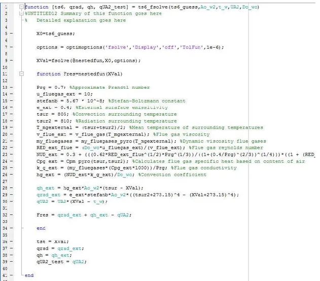
Figure 16 Example of an function with one output variable which depend on one input variable The function of figure 17 use another type of feature, called fsolve.
fsolve is a function which has the possibility of calculating un-linear equations or equation systems.
Figure 17 is a unique case of this study due to the use of fsolve but use the same principle of returning an output while being dependent on several inputs. The fsolve work by having a guessing value “X0” from which XVal will be the final answer of the function. That is the surface temperature of the pyrometer (ts6)
Fres is the equation that is being solved which is dependent on the rest of the syntax observable in figure 17. Fsolve work by solving this equation = zero which is why there is a tolerance level assigned. Of this function Fres = qrad_ext + qh_ext – qUA2 which is the sum
Xval = fsolve(@nestedfun,X0,options) state that the function called nestedfun(=Fres) is the target of equation to be solved with the initial guess of X0, options determine the that the feature fsolve is to be used with a accuracy of 0,00001.
Figure 17 Example of a function script which return several outputs and depend on several input variables
(The Mathworks, Inc, 2016c) fsolve source ; (The Mathworks, Inc, 2016d)
4.4.3
Data import
This feature is used in correlation with linear interpolation in this study. Previously stated interpolation equations are used in conjunction with the stated functions, what differ from these is the use of importing tables directly into MATLAB and then interpolating while using the function feature.
Import of data is accomplished by using syntax designated as “fopen” , “fclose” and “fscan” “fopen” will open up the .txt file into MATLAB. “fscan” will scan the text file and create a matrix corresponding to the created layout of the file. “fclose” will then after completed