A Freundlich-based model for prediction of pH-dependent sulfate adsorption in forest soil.

TRITA-LWR Degree Project

A

F

REUNDLICH

-B

ASED

M

ODEL FOR

P

REDICTION OF P

H-D

EPENDENT

S

ULFATE

A

DSORPTION IN

F

OREST

S

OIL

Muhammad Akram

©Muhammad Akram 2015

Degree Project for the master program in Environmental Engineering and Sustainable Infrastructure

Ground water chemistry

Division of Land and Water Resources Engineering KTH Royal Institute of Technology

SE-100 44 STOCKHOLM, Sweden

Reference should be written as: Akram, M (2015) “A Freundlich-based model for prediction of pH-dependent sulfate adsorption in forest soil” TRITA-LWR Degree Project 15:22

SUMMARY IN

S

Den starka industrialiseringen i Europa efter andra världskriget medförde att stora mängder SO2 och NOx släpptes ut i samband med förbränning av fossila

bränslen. De svenska skogsekosystemen påverkades av utsläpp av SO2 följt av

depostion av H2SO4. Detta medförde att skogsmarkens förråd av sulfat (SO42-)

ökade. Denna masteruppsats studerar adsorptionen av SO42- i podsolers

Bs-horisonter i svensk skogsmark. Jordprov från fem olika provtagningspunkter studerades, och resultaten visar att jordarna förmår ackumulera varierande mängder av adsorberat SO42- beroende på förändringar i jämviktskoncentration

och pH-värde. Den här studien visar att mängden adsorberat SO42- (mmol/kg

jord) ökar med ökande jämviktskoncentration SO42- (mmol/l) och med

sjunkande pH-värde. Detta observades i jämviktsexperiment på laboratoriet. För att beskriva resultaten utvecklades en modell för att kunna förutsäga förrådet adsorberat SO42- (mmol/kg) i de olika jordproverna. En

Freundlichbaserad modell användes, och mängden adsorberat SO42- (mmol/kg)

beräknades som funktion av pH och av jämviktskoncentrationen SO

42-(mmol/l) i marklösningen. Den utvidgade Freundlichmodellen optimerades på tre olika sätt: (1) genom obegränsad optimering då alla tre koefficienter Kf, m och y optimerades samtidigt, (2) genom begränsad optimering då värdet för y, som betecknade den mängd vätejoner (H+_{) som bands till ytan för varje}

adsorberad sulfatjon, sattes till 2, och (3) genom en förenklad tvåpunktskalibrering, där en begränsad optimering gjordes för endast två prover från varje jord användes för varje jord. Determinationskoefficienten R2_, samt värdena för de optimerade koefficienterna, var mycket likartade för obegränsad och begränsad optimering, beroende på att det optimerade värdet för y var nära 2 för 4 av 5 jordar. Värdet för R2 översteg 0,96, och 0,99 för de två jordar (Risbergshöjden B och Kloten Bs) som hade högst kapacitet att adsorbera sulfat. Även den förenklade tvåpunktskalibreringen gav goda anpassningar med värden för de optimerade koefficienterna som låg nära de som fanns när hela mängden datapunkter användes i modellkalibreringen. Den förenklade tvåpunktskalibreringen ansågs vara den bästa optimeringsmetoden, eftersom den endast kräver två observationer för varje jord.

SUMMARY IN

E

The industrialization in Europe after World War II released the large amounts of SO2 and NOx during the combustion of fossil fuels. The Swedish forest

ecosystems were affected by discharges of SO2 followed by deposition of

H2SO4. This meant that the forest soil reservoir of SO42- were increased. This

master thesis study the adsorption of SO42- in podzolic Bs horizons of Swedish

forest land. The adsorption results of soil samples from five different sampling points show that the soils are able to accumulate varying amounts of adsorbed SO42- by depending on the change in the equilibrium concentration and pH.

This study shows that the amount of adsorbed SO42- (mmol/kg soil ) increases

with increasing equilibrium concentration of SO42- (mmol/l) and with

decreasing pH. This was observed in equilibration experiments in the laboratory. To describe the results, developed a model to predict reservoirs of adsorbed SO42- (mmol/kg) in the different soil samples. A Freundlich based

model was used, and the amount of adsorbed SO42- (mmol/kg) was calculated

as a function of pH and the equilibrium concentration of SO42- (mmol/l) in the

soil solution. The extended Freundlich model was optimized in three different ways: (1) by unconstrained optimization when all three coefficients Kf , m and y were optimized simultaneously, (2) by constrained optimization when the value of y, which signifies the amount of hydrogen ions (H+_{) bound to the surface}

together with each adsorbed sulfate ion, was set to 2, and (3) through a simplified two-point calibration, where a constrained optimization was made for only two samples from each soil. The coefficient of determination R2_{, and} the values of the optimized coefficients were very similar for the unconstrained and constrained optimization, as the optimized value of y was close to 2 for 4 of 5 soils. The value of R2 exceeded 0.96, and 0.99 for the two soils (Risbergshöjden B and Kloten Bs1) that had the highest capacity to adsorb SO42-. The simplified two-point calibration produced the values of the

optimized coefficients that were close to those obtained when the entire number of data points were used in the model calibration. Therefore the simplified two-point calibration was considered the best optimization method, since it requires only two observations for each soil.

ACKNOWLEDGEMENTS

First of all, I would like to thank my supervisor Prof. Jon Petter Gustafsson for accepting me as a master thesis student and gave me an opportunity to work under his guidance and supervision, apart from this fact, I got the opportunity to work with him on this interesting thesis subject. His suggestions on literature selection, guidance in performing experiments in the laboratory and report writing without which it would not have been possible to accomplish this thesis. I would also like to thank Charlotta Tiberg, a PhD student at the Swedish University of Agricultural Sciences Uppsala who provided soil samples and helped me by giving useful guidance and information about the soil sampling sites. I would also like to acknowledge the support and help given by Ann Fylkner and Bertil Nilsson during Ion Chromatography analysis and other experimental work at the Department of Land and Water Resources Engineering.

I would also give thank to Md. Annaduzzaman a PhD student at Division of Land and Water resources Engineering, who has helped to format the thesis report. He always sincerely motivated me during this whole period of thesis work.

I would also like to deeply oblige my parents, brothers and sisters for their continuous prayers, love and moral support.

A

S

Al Aluminum

Al3+ Aluminum ion

Ca+ _{Calcium ion}

CaSO4·2H2O Calcium sulfate dihydrate (Gypsum)

DOC Dissolved organic compound

Fe Iron

H+ Hydrogen ion

HNO3 Nitric Acid

IEAs International environmental agreements

K+ Potassium ion

Kf Freundlich coefficient

M Non-ideality parameter in Freundlich equation MgSO4 Magnesium sulfate

Mg+ Magnesium ion

N Nitrogen

NOx Nitrogen oxide

Na2SO4 Sodium sulfate NO3 2-Nitrate ion NH4 Ammonium OH- _{Hydroxyl ion}

R2 _{Coefficient of determination in regression equation}

SO2 Sulfur dioxide

SO4

2-Sulfate ion

USDA United state department of agriculture USEPA United state environmental protection agency WHO World health organization

T

SUMMARY IN SWEDISH ... III SUMMARY IN ENGLISH ... V ACKNOWLEDGEMENTS ... VII ABBREVIATIONS AND SYMBOLS ... IX TABLE OF CONTENTS ... XI

ABSTRACT ... 1

1. INTRODUCTION ... 1

2. BACKGROUND ... 2

2.1. FOREST SOIL SYSTEM ... 3

2.2. ABATEMENT IN ACID DEPOSITION ... 4

2.2.1. North America, Europe and eastern Asia ... 4

2.2.2. Sweden ... 5

2.3. ADSORPTION ... 5

2.3.1. Factors affecting sulfate adsorption in soils ... 5

2.4. MECHANISM OF SULFATE ADSORPTION... 6

2.4.1. Chemistry of sulfate adsorption ... 6

2.5. BACKGROUND OF STUDY ... 6

2.6. SCOPE AND OBJECTIVE ... 8

2.6.1. Importance of study ... 8

2.6.2. Scope ... 8

2.6.3. Objective ... 8

3. MATERIALS AND METHODS ... 8

3.1. SITE AND SOIL DESCRIPTION ... 8

3.2. PHYSICAL CHARACTERISTICS OF SOIL SAMPLES... 9

3.2.1. Phase separation and pH measurement ... 10

3.3. EXTRACTION OF INITIALLY ADSORBED SO42-... 10

3.3.1. Extraction of initially adsorbed SO42- by phosphate ... 10

3.3.2. Extraction of initially adsorbed SO42- by bicarbonate ... 12

3.4. MEASUREMENT OF THE SOIL MOISTURE CONTENT ... 12

3.5. SO42- MEASUREMENT ... 12

3.5.1. Calculation of added concentration of SO42- - C added ... 12

3.5.2. Calculation of initial concentration of SO42- present in soil- C init. ... 12

3.5.3. Calculation of dissolved concentration of SO42- - Caq ... 13

3.5.4. Calculation of sorbed concentration of SO42- – C sorbed ... 13

4. MODELING APPROACH ... 13

4.1. THE FREUNDLICH EQUATION... 13

4.1.1. Limitations ... 13

4.2. EXTENDED FREUNDLICH EQUATION ... 13

4.3. OPTIMIZATION STRATEGY ... 15

4.3.1. Unconstrained fit ... 15

4.3.2. Procedure of optimization ... 15

4.3.3. Constrained fit ... 16

4.3.4. Procedure of optimization ... 16

4.3.5. Simplified two-point calibration ... 16

4.3.6. Procedure of optimization ... 16

5. RESULTS AND DISCUSSION ... 17

5.1. INITIAL EXTRACTABLE SO42- PRESENT IN SOILS ... 17

5.3. FITTING THE EXTENDED FREUNDLICH MODEL FOR SULFATE ADSORPTION. ... 20

5.3.1. The proton co-adsorption stoichiometry - unconstrained fit ... 20

5.3.1. The proton co-adsorption stoichiometry - constrained fit ... 21

5.3.2. The proton co-adsorption stoichiometry- simplified two-point calibration ... 22

5.4. DISCUSSION ... 23

5.5. CONCLUSION ... 24

5.6. PRACTICAL SIGNIFICANCE OF THE MODEL ... 24

5.7. FUTURE RECOMMENDATION ... 24 REFERENCES ... 25 OTHER REFERENCES ... 27 APPENDIX I ... 29 APPENDIX II ... 31 APPENDIX III ... 32 APPENDIX IV ... 33 APPENDIX V ... 33

A

The period of industrialization after the second World War in Europe released SO2

and NOx by combustion of fossil fuels and contributed the formation of S and N compounds in the forest ecosystem. The Swedish forest soil systems were influenced by emissions of SO2 followed by H2SO4 deposition, consequently the pool of SO

42-had increased in the forest ecosystem. This thesis studied SO42- adsorption in a

podzolic Bs horizon soils taken from a Swedish forest soil system. The soil samples from five different sampling sites were collected and the results revealed different amounts of adsorbed SO42- in response to changes in equilibrium concentration and

pH. This study found that the amount of adsorbed SO42- (mmol/kg) increased with an

added equilibrium concentration of SO42- (mmol/l) and with a decreasing pH. This

was determined by equilibration experiments. Based on the results a Freundlich-based model was developed to predict the pool of adsorbed SO42- in the soil samples. The

model predicted the pool of adsorbed SO42- (mmol/kg) as a function of pH and the

equilibrium concentration of SO42- (mmol/l) in the soil solution system. The extended

Freundlich model was optimized in three different ways: by use of unconstrained, constrained and simplified two-point calibration. The results showed that the adsorption of sulfate in the Kloten Bs1 and Risbergshöjden B soils was higher as compared to the Tärnsjo B, Österström B, and Risfallet B soils. The coefficient of determination (R2) determined from an unconstrained fit of the extended Freundlich

model (with three adjustable parameters) for Risbergshöjden B and Kloten Bs1 were R2 =0.998 and R2=0.993. Nearly as good fits were found in a constrained fit with two

adjustable parameters when it was assumed that nearly 2 protons (2 H+_{) are}

co-adsorbed with one SO42- ion (Risbergshöjden B; R2=0.997 and Kloten Bs; R2=0.992).

The simplified two-point calibration with two adjustable parameters showed similar parameter values for all most soils and was considered the best optimization method of extended Freundlich model, especially as it requires only limited input data.

Key Words : Sulfate; Spodosols; pH Dependent Sulfate Adsorption; Extended Freundlich Model.

1.

INTRODUCTION

Acidic deposition which is mainly consists of sulfuric acid H2SO4, nitric

acid HNO3 and ammonium NH4+, are primarily derived from emissions

of sulfur dioxide SO2, Nitrogen oxide NO2 and ammonia NH3. These

compounds are largely emitted to the atmosphere by fossil fuel combustion and some agriculture activities (USDA and WHO, 2000). The fossil fuels combustion which is largely for power generation, for industrial production process and by households, provide a significant contribution to air pollution in urban areas and on a regional or wider scale (Mitchel et al., 1998; van Stempvoort, 1992). These emissions lead to acidic deposition in the form of sulfuric acid H2SO4, nitric acid HNO3

and ammonium NH4+ to ecosystems. Once acid compounds enter

sensitive ecosystems, they acidify soil and surface water by causing several ecological changes. In sensitive ecosystems, along with the acidification of soil and surface water, they affect nutrient cycling and impact the ecosystem services provided by forests. The atmospheric inputs of acidifying compounds derived from fossil fuel combustion hence disturb the soil ecosystem (Martinson et al., 2005). The long-term deposition of acidifying compounds on soil mainly results in three types of changes in soil: depletion of base cations, mobilization of dissolved inorganic aluminum and accumulation of sulfate and nitrogen (Krauskopf et al.; 1995; Schwartz et al., 2011).

The acidic emissions that contain compounds of sulfur (S) have oxidation states ranging from -2 (sulfide) to +6 (sulfate) (Prietzel et al., 2009). In the unsaturated zone of forest soils, S is present as the dominant and stable form of inorganic sulfate. Lower oxidation-state inorganic compounds are also present but in negligible quantities. Concentrations of sulfate (SO42-) in soils fluctuate throughout the year.

Because of variations in the balance between atmospheric inputs, decomposition of plants, plant uptake, leaching and microbial activity change SO42- concentration. In forest ecosystems, inorganic SO42- exists

in the form of soluble salts and adsorbed SO42- on the surface of

inorganic components of soil (Scherer, 2001; Eriksen, 2008).

Deposition of S and nitrogen (N) has led to acidification of soils and water in Europe. Different studies show that the soils are acidified by deposition of acidic emissions (Sverdrup et al., 1998). Deposition of S has however decreased substantially during the last decades and many acidified lakes show clear signs of recovery in eastern North America and Europe (Johnson, 1980). However, much of the problem with acidified soils and water still remains.

A decreased atmospheric deposition has altered the ecosystem of soils. The recovery of soil in response to decrease in deposition is delayed, a considerable time may be needed for recovery. The release of already adsorbed SO42- is not completed until a new steady-state, with respect to

current atmospheric inputs, is obtained. The delayed effect of SO

42-adsorption/desorption on the response of water systems to changes in the input acidity hence demands an accurate model to predict the recovery from acidification, and also to predict the delay of the soil chemical response to acidification due to altered forest management practices.

2.

B

In forest ecosystems acid deposition occurs as wet deposition (rain and snow), dry deposition (gases and particulates), and as cloud and fog deposition (Fig. 1). During wet deposition nitrogen oxides (NOx) and sulfur dioxide (SO2) are converted to nitric acid (HNO3) and sulfuric

acid (H2SO4) and deposited to the forest ecosystem.Deposition of SO

42-and nitrate (NO3-) by wet deposition are considered roughly equivalent

(Piirainen et al., 2002), whereas deposition of ammonium NH4+ in dry

deposition form is higher. Dry deposition of SO2 and NOx leads to the

deposition of acid after interacting with water in the forest ecosystem. NO3- and ammonium byproducts are used by forest vegetation to

support growth.

When sulfuric acid H2SO4 is deposited from the atmosphere into the soil

system, each molecule splits into two hydrogen ions (H+_{) and a}

negatively charged SO42- ion (Alewell et al., 1995). Soil is acidified by the

presence of H+ _{ion to replace base cations by ion exchange process.}

Furthermore, removal of displaced base cations acidify the soil system (Harrison et al., 1989). Moreover, SO42- is retained in the soil system. It is

retained in a variety of forms, such as adsorbed SO42- on soil particles

and as organic S. It is also leached from the soil and accompanied by an equivalent amount of base cations (Ca+_{, Mg}+ _{and K}+_{). When SO42- is}

retained by sulfate adsorption it delays the loss of base cations through leaching with SO42- and thus counters the acidifying effect of

atmospheric sulfur S deposition (Jung et.al., 2011). Understanding the association between the inputs of S and forest soil ecosystem chemistry

to appraise the response of forest ecosystem to acid inputs has been considered as critical (Mitchell et al., 1998; Barton et al., 1999).

Significant work has been done on the movement and reaction of SO

42-in soils. Some research has been performed to predict the adsorption of SO42- in forest soil system. According to Gustafsson (1995) and Karltun

(1997), the adsorption of SO42- in forest soil is a proton-buffering

process. This characteristic of SO42- adsorption delays the soil water

chemical response to changes in H+ _{and SO42- ions concentration of the}

permeating solution. This may, for example, reduce the immediate impact of atmospherically deposited H2SO4 when the latter has been

increased. This characteristic of sulfate adsorption is considered significant in reducing base cation losses (Gustafsson, 1995; Jung et al., 2011; Karltun, 1997). Base cations such as Ca+ _,K+ _{and Mg}+ _{leach from}

the soil with SO42- as a counter-ion. As a result of adsorption, SO42- is

retained in soil together with the base cations.

2.1. Forest soil system

The forest soil is a multifaceted heterogeneous medium consisting of solid phases that contain organic matter and different minerals (Gobran et al., 1998; Carlsson et al.; 1999). The soils that are developed in sandy glacial tills with low weathering rates are the most vulnerable part of the forest ecosystem to atmospheric acidic inputs (Gustafsson and Jaks, 1993). The retention of SO42- in soils is characterized by the particle

surfaces which contribute to adsorption. Soil particles with clay minerals

Fig.1. Emissions of sulfur dioxide SO2 and nitrogen oxide

compounds NOx into the atmosphere as a source of dry and wet acid deposition in soil. Source: USDA Forest Service (http://webcam.srs.fs.fed.us/pollutants/acidification)

and various oxide surfaces and solid phase humic substance usually possess large specific surface areas and reactive sites. Coarser particles such as sand possess very low surface area and hence are not important adsorbents (Gustafsson et al., 2007).

In humid regions the process of soil formation involves leaching of upper layer with accumulation of material in lower layers. In coarse textured glacial tills or sandy sediments, podzols are developed by the process of podzolisation. When organic matter present on the surface of soil releases abundant organic acids, the latter migrate downwards together with weathered Fe and Al in the soil profile (David et al.; 1983; Edwards, 1998; Alves et al., 2004; Gustafsson et al., 2007). During this process, organic acids form complexes with weathered Fe and Al and these are deposited in the subsoil horizon in the soil profile. In this subsoil horizon the complexes degrade, which leads to the formation of Fe and Al hydrous oxides.

Podzolised forest soils that contain Fe oxide and poorly crystalline aluminosilicate in the B horizon are important for SO42- adsorption. The

surfaces of these Fe and Al hydrous oxides serve as adsorbents for SO

42-especially under low pH conditions. SO42- adsorption in forested soil

systems is dependent on pH, quantity of Al and Fe hydroxide, organic matter and concentration of sulfate present in the soil system (Jung et al., 2011). In acidic soils, SO42- is adsorbed to the surface of amorphous iron

and aluminum oxide and hydrous oxide.

SO42- in Swedish forest soils is adsorbed somewhat unevenly. The spodic

B horizon has the maximum number of positive charges ions in the form of Fe and Al (hydr)oxides. Therefore in this horizon, and when organic carbon is low, SO42- is adsorbed to a significant extent (Grerup et al.;

1987; Gustafsson, 1995).

2.2. Abatement in acid deposition

The abatement in acid deposition in various regions of the world as compared to Sweden can be seen as,

2.2.1. North America, Europe and eastern Asia

The SO2 emissions have declined during the last decade in Europe and

North America due to implementation of international laws, policies and agreements (i.e. IEAs) on the reduction of S (Finus et al., 2003), but instead a rapid increase have been observed in areas of world which have high economic growth such as south-east Asia (Akselsson et al., 2013). Since 1970, the deposition level has decreased by as much as two thirds in Europe (Akselsson et al., 2013; Martinson, 2003). Already in 1984, it was observed that emission of SO2 and SO42- deposition had declined by

between 38 and 82 % in Europe and by 52 % in the United States (Johnson, 1984). Additionally, emissions of NOx and nitrogen deposition show a slighter decline of 17 to 20 %. According to the literature, in Europe, in 1980 the SO2 emissions was recorded as 55 Mt

(million ton) but this level decreased to 41 Mt (million ton) in 1990. It is noticed that the mean annual pH of the precipitation in eastern North America and Europe is in the range of 3.0 to 4.7 (Chesworth, 2008; Johnson, 1984).

On the other hand in the Asian-Pacific region emissions in 1990 reached about 35 Mt and are expected to increase rapidly. The effect of widespread acid deposition due to sulfur emission may have decreased in Europe but it is highly likely to increase in the Asian developing countries (WHO, 2000).

Acid deposition in north-east Asia has increased hastily in the past decade because of industrial growth and will most likely exceed stages noticed previously in the most polluted area of central and eastern Europe (Cole et al., 1997; Zhang, 1996). Consequently, the increase in emissions is a threat to sustainable forest ecosystems and a question of concern to take account of reduction in emissions(Ishiguro et al.; 2011).

2.2.2. Sweden

In Sweden, the decrease in the deposition of SO42- and H+ due to the

restriction (due to implementation of Environmental Protection Act 1969) of sulfur emissions started during the 1970s. They decreased considerably during the last decade (by following the targets of the Helsinki protocol in 1985 to reduce S emissions, the Oslo protocol in 1994 for further reduction S emissions, and the Gothenburg protocol in 1999 to abate acidification, eutrophication and ground level ozone) and now it is at level below that recorded in the mid-1950s. The continual decrease of the deposition resulted in an improved status of the water quality in forested catchments in Sweden (Fölster et al., 2002). However, the SO42- concentration in the forest ecosystems and surface waters of

south-west of Sweden has not decreased to the extent that could be expected from the decreased acid deposition. During the period of deposition decrease the desorption of already adsorbed sulfate acts as a buffering mechanism in forest soils. Depending on the soil properties, there may be a long delay between the decreased input of acid and the chemical recovery(Nömmik et al.;1998; Jönsson et al.; 2003).

2.3. Adsorption

SO42- and other anions such as phosphate, arsenate and molybdate

adsorb on the surface of adsorbents present in the soil. These anions are adsorbed through a reaction between the adsorbate (anions) and the surface of a solid adsorbent (Fe and Al oxide in soils) that involves ligand exchange (Selim et al.; 2004; Belyazid et al.; 2006; Gustafsson et al., 2007; Sokolova et al.; 2008).

2.3.1. Factors affecting sulfate adsorption in soils

The pH and the equilibrium concentration are two important factors that govern the adsorption of SO42- ions. The pH value is considered to be

the most important parameter. The reason is that the surface of adsorbent usually possesses variable charge and therefore the electrostatic forces of attraction are also variable and depend on the pH value. For example, SO42- is adsorbed more strongly at low pH on the

variable positively charge surfaces of Fe and Al hydrous oxides in soils. At high pH a negative charge occurs on the surface, hence cations are adsorbed more strongly at high pH (Rao, et al.; 1984; Sharpley, 1990; Stanko et al.; 2008).

In certain cases, the adsorption of the ion itself affects the pH values in the surrounding environment. When one SO42- ion is adsorbed to the

surface of Fe oxide as a surface complex, it decreases the charge of oxide surface by a value of 2. To compensate for this large change in charge, H+ ions and to some extent other cations are bound on the oxide surface

(Gustafsson, 2007; Karltun, 1997; Gustafsson, 1995)

The effect of ionic strength changes the number of co-adsorbed monovalent cations during sulfate adsorption on the surface of oxide surfaces in soil. At high ionic strength i.e. under conditions of high salinity this value is about 1, because 1 H+ _{is needed to protonate the}

surface for every sulfate ion being adsorbed. At low ionic strength, the number of co-adsorbed protons is nearly equal to 2 (Gustafsson, 1995).

2.4. Mechanism of sulfate adsorption

Sulfate is retained in the soil system by varying mechanisms. The main adsorption mechanism is called ligand exchange. In this specific adsorption mechanism SO42- is associated with metal (hydr) oxides of Fe

and Al present in the soil system by displacing OH- _{anions or H2O.}

During specific adsorption, the surface also accepts or donates protons, for the reasons stated in the above section. During the adsorption of SO42- on Fe and Al hydrous oxide surfaces, the sulfate anion accepts a

proton from the positive site of Fe and Al hydrous oxide surface (M-OH2+ where M= Fe or Al) and create monovalent HSO4-. This

monovalent ion replaces a OH- ion without creating additional negative

charge on the surface (Sjöström, 1993; Gustafsson, 1995; Zhang et al., 1996; Karltun, 1997; van Hees et al.; 2000).

The adsorption process of sulfate removes the acidity of soil solution and during desorption process acidity is released. Due to this, the recovery of soil is also delayed.

2.4.1. Chemistry of sulfate adsorption

Adsorption of SO42- results in the displacement of –OH ligands from

oxide:

Oxide-OH+SO4-2 Oxide-SO4-+OH- (1)

When an -OH from the metal (hydr)oxide is replaced, the surface charge decreases, which facilitates cation exchange. In reality, the replacement usually occurs in two steps: (i) H+ _{ions are sorbed, and (ii) SO42- ions}

bind by replacing -OH2+. Reaction (1) may therefore more accurately be

written as follows:

Oxide-OH+H+_{+ SO42- Oxide-SO4-+H2O (2)}

The release of water changes the charge from positive to negative on the site. These equations show that SO42- adsorption and the cation

exchange capacity may increase at the same time (Gustafsson, 1995; Karltun, 1997; Martinson et al., 2003; Goldberg, 2005 ).

Another related way to understand SO42- adsorption is by surface

complex formation theory (Gustafsson, 1995). According to this theory, sulfate ions adsorb onto Fe and Al hydrous oxides as outer- and inner-sphere complexes. The adsorption of SO42- as an inner-sphere surface

complex means that adsorption of SO42- changes the net charge on the

oxide surface. The electrostatic non-specific type of adsorption creates outer-sphere surface complexes and it balances the positive charge surface of the metal oxides. On the other hand, adsorption of SO42- as

inner-sphere complexes is stronger.

2.5. Background of study

This thesis takes its starting point in the modeling approaches of Gustafsson (1993 and 1995), Karltun (1997), Martinson (2003), and Gobran et al. (1998).

Gustafsson (1995) modeled pH-dependent sulfate adsorption in the Bs horizons of podzolised soils. He assumed that ̴ 2 H+ _{ions are consumed}

for every SO42- ion during adsorption. It was accomplished by sequential

leaching process with use of magnesium sulfate MgSO4. Use of acid until

pH 4.4 was reached facilitated determination of the SO42- adsorption

capacity in soils.

>MOH2(H20)n++SO42-+H+ >MOH2(H20)n+HSO42- (3)

The basic adsorption reaction of SO42- (equation 3) was used to predict

empirical model. This was tested in a Temkin isotherm approach in which the amount of adsorbed sulfate was assumed to be linearly related to log-transformed values of SO42- and H+. Further it was assumed that

the soil systems had very low ionic strength so that the value of y (the proton co-adsorption stoichiometry, i.e. the number of H+ that

accompanies every SO42- ion) is close to 2. This means that an extra H+

is adsorbed in the basic reaction and that the sulfate adsorption reaction can be viewed as the adsorption of H2SO4. Hence in this approach, the

adsorption of sulfate ion SO42- was assumed to be linearly related to the

term 2pH + pSO4, where pSO4 is the negative log of the dissolved

sulfate concentration.

Similar studies were made by Karltun (1997), although he used a surface complexation model approach to describe his data. He compared the surface complexation of SO42- and H+ between goethite, gibbsite and a

soil material from a podzol B horizon. He used the diffuse layer model and found that a model with only one SO42- surface species and no H+

ion explicitly take part in the adsorption reaction provided the best prediction of adsorption. He found that associated H+ co-adsorption

occurs during SO42- adsorption and by this the neutralization in the inner

layer the surface potential is decreased. He also performed his experiments under different pH, ionic strength and SO42- concentrations

to determine the y value, which was found to vary with pH and SO

42-concentration and with the ionic strength. His experimental work determined the y as being close to 1 at high ionic strength (0.1 M) but at low ionic strength (0.001 M) y was in the range of 1.5 to 1.7.

Courchesne & Hendershot (1989) measured the adsorption and desorption of SO42- to/from some podzolic soils of the southern

Laurentians in Canada as a function of pH and used six podzolic soils (Hermine B, Coniferous B, Laflamme 1 B1, Laflamme 1 B2, Laflamme 2 B1 and Laflamme 2 B2) of two forested watersheds of southern Laurentians. The effect of soil solution pH on SO42- of podzolic soils

was determined. They used four simple adsorption equations i.e. the Gunary equation, Freundlich equation, Langmiur equation and Temkin equations and observed SO42- adsorption and desorption as a function of

pH and initial sulfate concentration. They observed an increase in SO

42-adsorption with decreasing pH to a maximum 42-adsorption at pH 3.8 to 4.2. They could also relate the amount of adsorbed SO42- and total native

SO42- to the total oxalate extractable Al contents of soils. They found the

Gunary equation to produce the best fits to the soil data (R2_=0.999, R2_{=0.995, R}2_{=0.993, R}2_{=0.999, R}2_{=0.994 and R}2_{=0.999 respectively) of} each six soils as compared to Freundlich equation (R2=0.983, R2_=0.977, R2_{=0.987, R}2_{=0.972, R}2_{=0.980, and R}2_{=0.948 respectively).}

Martinsson et al., (2003; 2005) parameterized, evaluated and modeled the adsorption of SO42- by an isotherm in which it was assumed that SO

42-adsorption is fully reversible and depends on the concentration of SO

42-as well 42-as the soil solution pH. The isotherm they used w42-as in fact an extended Freundlich equation, which is described in detail below in chapter 4. The adsorption model was implemented in the dynamic multilayer soil chemistry model SAFE. The batch experimental work was performed at different pH and SO42- concentrations. In this research the

model was evaluated by applying to the roof covered catchment at Lake Gårdsjön in the south west of Sweden.

2.6. Scope and objective

2.6.1. Importance of study

As the increased deposition of acidic compound in soil after WW II in Europe increased the acidity and the amount of adsorbed SO42- in forest

soil. After the implementation of S emission abatement practices, the deposition of acidic compounds in soil is decreased. The response of reduction in emissions and acid deposition in soil is not the same. There is a lag of time to recover from acidity in soil. The adsorbed SO42- under

reduced acid deposition conditions will continuously release acidity (H+)

and leachable SO42- to the soil solution. This action of desorption has

delayed the soil water chemical response to changes in the H+ _{and SO}

42-ion concentrat42-ions of the permeating solut42-ion.

To facilitate correct dynamic models for acidification recovery it is important to develop a robust model for the prediction of the adsorbed pool of SO42-. In this thesis work different experiments have been

performed to investigate the extent of adsorption in five different soil samples from Swedish Podzols. The results of the equilibration experiments were used to optimize the model. Ultimately, the following questions will be answered:

1. Can the extended form of Freundlich equation predict the adsorbed pool of SO42- in forest soil?

2. Which optimization approach is the best considering the requirement to use as few samples as possible to bring down analysis costs?

2.6.2. Scope

This thesis presents an attempt to develop a model to predict the pool of adsorbed SO42- in the Bs horizons of podzolic Swedish forest soils. Such

a model is of interest due to the delayed effect sulfate adsorption/desorption has on the response of water systems to changes in the input acidity. Hence an accurate model is needed to be able to predict the recovery from acidification, and also to predict the delay of the soil chemical response to acidification due to altered forest management practices.

2.6.3. Objective

The objective of this study is therefore to calibrate a Freundlich equation for the prediction of SO42- adsorption using experiments data in which

the adsorption of SO42- is studied as a function of pH and dissolved

equilibrium concentrations of SO42-. In the calibration, five soil samples

were selected from well-developed spodic B horizons in five different locations from Swedish forest soils.

3.

M

M

3.1. Site and soil description

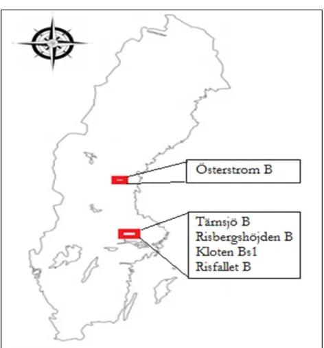
The soil samples used in the investigation were sampled from five different locations. The four soil samples (Tärnsjö B, Risfallet B, Risbergshöjden B and Kloten Bs1) were sampled from the Bergslagen area which is situated west of Uppsala, and one soil (Österström B) was from Holm, to the west of Sundsvall (Fig. 2). The samples were collected in May and July 2012. All sampled soils are Podzols (Table 1) and the samples were collected from the upper part of the B horizons (Bs1). The exact sampling depth of each soil was different (Table 2) and varied between the locations.

3.2. Physical characteristics of soil samples

The physical characteristics of soil samples were determined. The soils varied in texture, particle size, moisture and color (Fig. 3). As these soil samples were taken from the spodic B horizons, they had reddish-brown color due to the presence of Fe, Al and humic substances.

The Tärnsjö B soil sample was dark brown, less moist and a little coarser in texture. In physical appearance, the Risfallet B soil was dark and more moist than Tärnsjö B. Risbergshöjden B and Österström B were more fine, dark and with much moisture present in soils. The Kloten Bs1 soil was mixed with clay and was much moist and sticky in nature.

The suspension of soil samples were prepared according to the recipe (Appendix I) by adding 2 g of soil, then adding volume of water as per the recipe, then adding 0.10 mM MgCl2 as background electrolyte and

lastly SO42- (using the appropriate amount of Mg2+ and H+ as counter

ions) was added at the amounts specified in the recipe. Each suspension was prepared in duplicate. After that the lid was tightly attached to all centrifuge bottles and placed in a rack. The rack with 40 centrifuge bottles was inserted in the end-over-end shaker and was fixed tightly. The rack along with bottles was shaked for 6 days to reach equilibration at room temperature (21o_{C). After 6 days of shaking, the bottles were}

removed from the end-over-end shaker and placed in the centrifuge for centrifugation at 3500 rpm for 15 minutes to separate the soil and solution phases. After centrifugation, the bottles were removed from the centrifuge carefully to avoid phase mixing and placed at room temperature to cool down for a while.

Fig. 2. Map to indicate the location of sampling sites of Tärnsjö B, Risbergshöjden B,.Kloten Bs1, Risfallet B and Österström B soils.

3.2.1. Phase separation and pH measurement

The bottles were transferred to the pH meter. A Radiometer PHM 93, Copenhagen pH meter was used. 40 scintillation bottles (20 ml) were prepared and marked to store the filtrate of each equilibrium suspension accordingly. The pH meter was calibrated according to standard procedures. After this, 5 ml of the supernatant was taken by using a Biohit pipette, transferred to the pH measurement bottle and the pH measurement was started (the results of the pH measurements for each series are shown in Appendix II). The remaining phase-separated supernatant (15-20 ml) was filtered using an Acrodisc PF 32 mm0.8/0.2 µm membrane syringe filter (Pall Corp., Washington, NY, USA) and the filtrate was transferred into a scintillation bottle marked with the appropriate sample number.

3.3. Extraction of initially adsorbed SO

2-To be able to know the amount of adsorbed SO42- in equilibrium with a

certain dissolved SO42- concentration, the amount of adsorbed SO42- is

determined by calculating initially adsorbed SO42- and additionally

adsorbed SO42-.

For the data treatment it was required to quantify the initially adsorbed amount of SO42- in the soil samples. This was done in two ways: by the

phosphate and by bicarbonate extraction.

3.3.1. Extraction of initially adsorbed SO42- by phosphate

For the purpose of determining initially adsorbed SO42- in soil, an initial

solution of 20 mM NaH2PO4 was prepared. Extraction of initially

adsorbed SO42- was done to all five soil samples individually. For each

soil the extractions were carried out in duplicate. For this purpose, 10 centrifuge bottles were prepared by washing with acid and deionized water, and then dried. All centrifuge bottles were marked according to the soil samples consequently. After this, 2 g of moist soil was added to a centrifuge bottle. Then 20 ml of 20 mM NaH2PO4 was added. The lid

was attached to the bottle and placed into the rack. The rack was adjusted tightly to the end-over-end shaker and shaken for 24 hours at

Table 1. General properties of Tärnsjö B, Risbergshöjden B, Österström B, Kloten Bs1 and Risfallet B sampling sites.

Site Land use Vegetation Topo-graphy Ground-water table Drainage

Risfallet Forestry Coniferous forest,

birch. Moss, grass Hilly > 80 cm

Rather well drained Tärnsjö Forestry Coniferous forest (pine). Moss, lichen Flat > 80 cm Well drained Risbergs-höjden Forestry Coniferous forest. Lichen, lingon/blueberry Hilly > 80 cm Well drained Kloten Forestry Coniferous forest. Grass, heather, moss Slightly sloping > 80 cm Well drained Österström Forestry Confierous forest. Lichen, lingon/blue berry Hilly > 80 cm Well drained

Table 2. General properties of Tärnsjö B, Risfallet B, Risbergshöjden B, Österström B and Kloten Bs1 soils.

Soil Hori-zon Depth (cm below surface) pH (0.01 M CaCl2) Oxalate-Fe (mmol /kg) Oxalate -Al (mmol /kg) Tärnsjö Bs1 2-16 4.88 45 118 Risfallet Bs1 7-15 4.24 151 265 Risbergshöjden Bs1 4-13 4.39 119 534 Österström Bs1 5-15 4.13 85 166 Kloten Bs1 14-24 4.73 114 647

Fig. 3. Images of (a) Tärnsjö B; (b) Risbergshöjden B; (c) Österström B; (d) Kloten Bs1 and (e) Risfallet B soil samples before equilibration experiments.

room temperature. After shaking, bottles were removed and placed in the centrifuge. The centrifugation was at 3500 rpm for 15 minutes. After centrifugation bottles were removed carefully to avoid phase mixing. After this, filtration of the extracts was done by using Acrodisc PF 32 mm 0.8/0.2 µm membrane syringe filters attached to a plastic syringe. The filtered extract of each soil solution was stored in 20 ml scintillation bottles.

3.3.2. Extraction of initially adsorbed SO42- by bicarbonate

For the extraction of initially adsorbed SO42- by bicarbonate, 40 mM

NaHCO3 was prepared. The same five moist soils were used to extract

initially adsorbed SO42-. The same procedural steps were followed as for

extraction by phosphate to prepare suspensions, shaking, centrifugation and filtration.

3.4. Measurement of the soil moisture content

The results for SO42- adsorption were reported in terms of sulfate

adsorbed per gram weight of dry soil. For this reason it was required to measure the moisture content of soil samples. The moisture content of each soil sample was measured as follows: First the oven was set at 105o_{C. Five clean and dry porcelain crucibles were weighted and was}

noted as the initial weight of the crucible. 3 to 5 g of soil sample was added to the porcelain crucible and placed again on a balance, the weight of moist soil and crucible was noted (up to 3 decimals). After this, the crucible with soil sample was placed in the oven to dry for 24 hours. After drying for 24 hours the crucible was removed from the oven and was transferred carefully and immediately to an excicator to let it cool down for 20 minutes. After this, the sample was taken out from the excicator and weighed exactly (three decimals). This same procedure was adopted for each soil, the results of soil moisture content are in Appendix IV.

3.5. SO

measurement

The filtrates stored in the scintillation bottles were analysed for SO

42-using ion chromatography. A Dionex DX-120 instrument (Dionex Corp., Sunnyvale, CA, USA) was used to measure the amount of dissolved SO42- (mg/l) for all samples from the batch equilibrations and

from the extractions.

3.5.1. Calculation of added concentration of SO42- - C added

The concentration of added SO42- was calculated by using the recipe for

each suspension preparation. However, it needed to be corrected for (a) a slight deviation of 7 % between the nominal concentration and the final one, as found after repeated IC analysis of the stock solution, and (b) the amount of water present in the field-moist soil (which causes a slight dilution). The resulting value of Cadded was expressed in µmol/l.

3.5.2. Calculation of initial concentration of SO42- present in soil- C init.

The calculation of initial concentration of SO42- present already in the

soil was done with the help of phosphate extraction. During extraction of initial SO42- by phosphate the filtrate extract was analysed by ion

chromatography. The L/S (liquid to solid ratio) was calculated with the help of the moisture content of each sample. The calculated L/S value was used to calculate the experimental SO42- (mmol/kg of SO42-). After

this these values given in mmol/kg were converted to initial concentration Cinit. of SO42- µmol/l present in the samples.

3.5.3. Calculation of dissolved concentration of SO42- - Caq

The calculation of dissolved concentration of SO42- was done by taking

the average of SO42- dissolved (mg/l) in duplicate samples measured by

ion chromatography for each soils, divided with the average value of dissolved SO42- (mg/l) with the molecular weight of SO42- (96.06 g/mol).

Then this value was multiplied by 1000 to obtain the units of Caq in µmol/l.

3.5.4. Calculation of sorbed concentration of SO42- – C sorbed

The concentration of sorbed SO42- was calculated by using the values of

C init, C added and C aq. For this, first the general calculations were done by using the relationship of these above mentioned concentrations as, Cinit+(Cadded - Caq) µmol/l. The result obtained was in µmol/l, it was converted to µmol/kg by multiplying L/S derived by using soil in equilibration experiments.

4.

MODELING APPROACH

4.1. The Freundlich equation

The basic Freundlich equation is the derived form of linear KD model

with adjustable parameters m and Freundlich coefficient Kf . The general form of Freundlich equation is as:

(4) The non linear relationship between adsorbed concentration of solute (sulfate) Q (mol/kg) and dissolved concentration C (mol/l) gives a slope less than 1.

4.1.1. Limitations

This simple form of Freundlich equation is useful to fit the adsorption data only at fixed pH. In addition it cannot explain the competition of ions.

As we are interested in simulating pH-dependent SO42- adsorption, there

is a need to extend the simple Freundlich equation. Through the extended Freundlich equation, the major drawbacks of the simplistic equation can be resolved.

4.2. Extended Freundlich equation

To overcome the limitations of simple Freundlich equation, it can be extended by including extra terms of activity of H+ _i.e.{H+_{} and}

concentration of competing ions with adjustable parameters. The version of the extended Freundlich equation to be used in this thesis can be expressed as:

(5)

The logarithmic form of the equation can be written as

(6) (7) where Q represents the amount of adsorbed sulfate in mol/kg, C is the equilibration concentration of sulfate measured in mol/l, Kf is the Freundlich coefficient measured as the y-intercept in Freundlich equation, and m is the slope.

E quation (7) implies that we can plot (Fig. 4) adsorbed SO42- as

log Q (mol/kg) on the y axis against dissolved SO42- as log C (mol/l) and

Fitting the extended Freundlich equation for SO42- adsorption:

During SO42- adsorption onto hydrous oxides of Fe and Al, a certain

number of H+ _{ions is co-adsorbed (i.e. the number of H}+ _{ions that}

accompany each SO42- ion during adsorption) to prevent excess charge

development on the surface of minerals (hydrous) oxide. Hence, we can write the SO42- adsorption reaction as follows:

SO42- + y H+ ads-SO4 (8)

where y is the number of protons e.g. number of H+ _{co-adsorbed to}

prevent excess charge development. It varies depending on the ionic strength. At high ionic strength, i.e. when the salinity is high, the number of co-adsorbed H+ _{needed to protonate the mineral surface for SO42- to}

adsorb is close to 1. With a decrease in salt content at low ionic strength I the number of co-adsorbed proton H+ _{is close to 2. We may derive the}

hypothetical equilibrium constant of the above equation as:

=K (9)

We may then express this in terms of the extended Freundlich equation, in which the exponent m describes the non-ideality of the dissolved components. Furthermore, the SO42- ion activity SO42-} is replaced with

the term total dissolved SO42- i.e. [SO42-]t as is customarily the case in the

Freundlich equation, and we get,

Fig. 4. Freundlich equation isotherm expressing the amount of adsorbed sulfate log Q (mol/kg) as a function of equilibrium concentration log C (mol/l).

ads-SO4 = Kf ( SO42- ]t{H+}y m (10)

where ads-SO4 is expressed in mol/kg and represents all adsorbed SO42-.

It includes the amount of SO42- sorbed during the experiment and

initially present adsorbed SO42-.The sorbed SO42- is calculated by

subtracting the concentration of dissolved SO42- from the added

SO42(mmol/kg). Kf and m are the coefficients of the Freundlich equation

(the y intercept and slope respectively after log-log transformation). The total dissolved sulfate SO42- ]t is expressed in mol/l.

Equation (10) can be written in the logarithmic form as:

log ads-SO4 = log Kf + m (log SO42- ]t + y log {H+}) (11)

as we know pH = -log{H+_}

log ads-SO4 = log Kf + m (log SO42- ]t – y(pH)) (12)

The plot of log ads-SO4 on the y axis against log SO42- ]t – y.(pH) on the

x axis should provide a straight line according to the extended Freundlich equation, after adjustment of the value of y to an optimum value. In practice during the calculations, the trendline tool in the Microsoft Excel was used to provide the best fit using linear regression. For the unconstrained fit (section 4.4.2), a trial-and-error method was used to simultaneously arrive at optimum values of y, Kf and m.

4.3. Optimization strategy

The optimization of extended Freundlich equation (12) was done in three different ways:

• Unconstrained fit. In this method, the values of y, Kf and m were optimized simultaneously without any constraints on their values. • Constrained fit. A constant value of y was assumed, which means that

only Kf and m were optimized.

• Simplified two-point calibration. This method also used a constant value of y, but only two data points with different pH and [SO42-]t were

used in the optimization.

During optimization, the data of each soil was processed individually.

4.3.1. Unconstrained fit

By definition, the unconstrained fit function is the fit of data by means of all three adjustable parameters y, Kf and m. To optimize the extended Freundlich equation (Equation 12) the unconstrained fit requires a wide range of pH values and dissolved sulfate concentrations to be successful, because otherwise different combinations of y, Kf and m can equally well describe the data.

4.3.2. Procedure of optimization

During optimization the following procedural steps were adopted, • Calculation of the term log SO42-]t (mol/l) from the data set for each

individual soil.

• Calculation of log ads-SO4 (mol/kg).

• The use of relationship log SO42-]t – y(pH).

• Optimization of the value of y by the trial-and-error method. • log ads-SO4 was plotted as a function of log SO42-]t – y(pH).

• The trendline (linear) tool was used to produce the regression equation and R2 _{values (five decimal points).}

• The value of y was again optimized by the trial-and-error method to obtain a new value of R2_{, and the steps above were repeated until the} optimum combination of y and R2 _{values were found.}

• At this point the values of the slope (m) and the y-intercept (log Kf) were collected from the graph.

• The Freundlich coefficient Kf was calculated from log Kf.

4.3.3. Constrained fit

In the constrained fit the adjustable parameter y is selected as common value of 2. The value of 2 was chosen because it was thought to represent low-ionic-strength conditions as found in the forest soils acceptably well (Background section). The constrained fit has the advantage that optimization of only two parameters results in more robust estimates and thus it does not require such a large variation in pH and dissolved sulfate concentrations.

4.3.4. Procedure of optimization

During optimization following procedural steps were adopted,

• Calculation of the term log SO42- ]t (mol/l) from the data set for

each individual soil.

• Calculation of the term log ads-SO4 (mol/kg).

• The relationship of log SO42- ]t – 2pH was used.

• log ads-SO4 was plotted as a function of log SO42- ]t – 2pH.

• The trendline (linear) tool was used to produce the regression equation and R2 values.

• The slope m and the y intercept log Kf were taken from the regression equation.

• The Freundlich coefficient Kf was calculated from log Kf.

4.3.5. Simplified two-point calibration

In the simplified two-point calibration only two data points were selected from the data set and used in the optimization. By this method it was tested whether it was possible to select only two points from the data set and still be able to produce a reliable model. By using the simplified two-point calibration, the use of the extended Freundlich model will be much easier, because large sets of soils can be optimized with a limited number of observations.

4.3.6. Procedure of optimization

• From each soil data set, the duplicate samples according to the recipe with 0.1 mM MgCl2 only were selected. For example, for Tärnsjö B,

sample A1 and A2, for Risbergshöjden B, sample B1 and B2, for Österström B, sample C1 and C2, for Risfallet B, sample A27 and A28, and for soil Kloten Bs1, sample D1 and D2 were selected (Appendix V), and the average value of each duplicate sample were calculated.

• Selection of the pH value of each respective soil samples and calculation of average of each duplicate pH value.

• Similarly, selection of the dissolved sulfate value SO42- ]t (mmol/l)

and adsorbed sulfate values (mmol/kg) for each respective soil samples and calculation of the average and log of each duplicate dissolved sulfate and adsorbed sulfate values.

•

significantly in both pH and dissolved sulfate compared to the 0.10 mM MgCl2 samples. For example, for Tärnsjö B, sample A25

B,sample C25 and C26, for Risfallet B, sample A39 and A40, and for Kloten Bs1, sample D25 and D26 from the data set were selected (Appendix V) , and the average of each sample values were calculated.

• Again the average of pH values for each respective sample of highest SA solution were calculated.

• The dissolved SO42- value SO42- ]t (mol/l) and adsorbed SO

42-(mol/kg) for each respective soil samples were selected and the average and the logs of each duplicate dissolved SO42- and adsorbed

SO42- were calculated.

• The term log SO42- ]t – 2pH was used.

• A graph between log SO42- ]t – 2pH on the x axis vs log ads-SO4 on

the y axis was plotted.

• The trendline (linear) tool was used to the data of each soil to display the regression equation and R2.

• The values of the slope m and the y intercept log Kf were taken from regression equation.

• The Freundlich coefficient Kf was calculated from log Kf.

5.

RESULTS AND

DISCUSSION

Firstly, in this section the initially extractable adsorbed SO42- present in

each soil samples and correlation between initially adsorbed SO42- with

the amount of Fe and Al hydrous oxide as determined by oxalate extraction can be expressed as,

5.1. Initial extractable SO

present in soils

The initially adsorbed SO42- present in the soils extracted by phosphate

extraction is different in each soil. It may depend on the location of the sampling sites, depth, soil type, the nature of sampling site, and the type of forest ecosystem (Table 2). The initially adsorbed SO42- (Fig. 5)

present in the soil samples extracted by phosphate (sodium phosphate, NaH2PO4) shows that the extracted amount of SO42- in Risbergshöjden

B soil is high (4.55 mmol/kg) as compared to other soils. The second largest amount of SO42- initially adsorbed is in Kloten Bs1,

4.17 mmol/kg. Similarly, in Risfallet B, Tärnsjö B and Österström B, initially adsorbed SO42- extracted by NaH2PO4 is 1.30 mmol/kg,

0.78 mmol/kg and 0.61 mmol/kg respectively.

The high value of initially bound sulfate in Risbergshöjden B and Kloten Bs1 is well correlated (Fig. 6) with the amount of Fe and Al hydrous oxide as determined by oxalate extraction. The high amount of oxalate extractable Fe in Kloten Bs1 (114 mmol/kg) and oxalate extractable Al (647 mmol/kg) and in Risbergshöjden B (119 mmol/kg and 534 mmol/kg Fe and Al respectively) as compared to other soil provide evidence (Fig. 6) that Risbergshöjden B and Kloten Bs1 soils have high value of initially bound sulfate.

Fig. 5. The amount of initially adsorbed SO42- (mmol/kg) in the

Tärnsjö B, Risbergshöjden B, Österström B, Kloten Bs1, and Risfallet B soils.

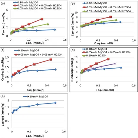
5.2. Sulfate adsorption isotherms

The sulfate adsorption isotherms (Fig. 7) of Tärnsjö B, Risbergshöjden B, Österström B, Kloten Bs1, and Risfallet B soils used in the study were determined by plotting the equilibrium concentration of sulfate (mmol/l) against the amount of SO42-

adsorbed (mmol/kg) in soil. Comparing the

highest amount of SO42- adsorbed (mmol/kg) in each soil, it is evident

that the soils differ in terms of their SO42- adsorption capacity. The

results for adsorption of SO42- (Table 3) show that the maximum

concentration of SO42- adsorbed in Tärnsjö B soil is 3.93 mmol/kg when

the pH was 4.71 and the dissolved SO42- concentration was

0.348 mmol/l.

The soil data plotted in Fig. 7 are the mean values of duplicate samples. The pattern of SO42- adsorption as a function of equilibrium

concentration for all levels of sulfate addition is the same for all soils.

Table 3. Amount of adsorbed SO42- after addition of 0.5 mM SO42-.

Soil Maximum SO4 adsorbed (mmol/kg) pH at maximum SO4 2-adsorption Tärnsjö B 3.93 4.71 Risbergshöjden B 8.25 4.45 Österström B 2.29 4.22 Kloten Bs1 9.26 4.65 Risfallet B 1.83 4.82

Fig. 7. Adsorbed SO42- (mmol/kg) during the experiment as a

function of equilibrium concentration of SO42- (mmol/l) for (a)

Tärnsjö B; (b) Risbergshöjden B; (c) Österström B; (d) Kloten Bs1; (e) Risfallet B.

The values for adsorbed SO42- include the initial sulfate adsorbed in each

soil. The difference in the amounts of adsorbed SO42- in each soil is well

correlated with the amount of sulfate that was initially adsorbed, and maximum adsorbed SO42- with oxalate-extractable Fe+Al (Fig. 6). It is

evident from Fig. 6 that SO42- adsorption increased with the increase in

the concentration of SO42-, but also that the equilibrium pH had a strong

effect on the result. There is illustrated that the amount of sulfate adsorbed (mmol/kg) is increasing with the increase in amount of sulfate in equilibrium solution at any given equilibrium pH value.

The trends of the isotherm of each soil (Fig. 7) explain the concept of adsorption of SO42-. The general tendency of an increase in sulfate

adsorption with a decrease in pH is understandable. At low pH, the soils possess more positive surface charge. The different sulfate adsorption behavior of different soils can be attributed partly to differences in competitive adsorption of other anions and organic compounds in the soil.

5.3. Fitting the extended Freundlich model for sulfate adsorption.

be expressed by Unconstrained, Constrained and Simplified Two point fits as;

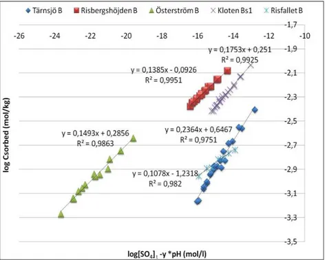
5.3.1. The proton co-adsorption stoichiometry - unconstrained fit

When the sorption data for all five soils sample were plotted between log SO42- ]t – y(pH) on the x axis and log ads-SO4 on y axis by using

unconstrained fit Freundlich equation (Fig. 8), it showed that the adsorption data were well described for all soils. The co-adsorbed number of proton y during SO42- adsorption in each soil (Table 4) was

different but ideally it should be close to 2, because of the low ionic strength in these systems.

From Fig. 8 it seems that the extended Freundlich model showed an excellent fit to the data particularly at lower concentration.

From the unconstrained fit (Table 4) it seems that Risbergshöjden B and

Kloten Bs1 showed the best fit (y= 2.44, R2_{= 0.995, and y=2.05, R}2 ₌ 0.993 respectively) followed by Österström B, Risfallet B and Tärnsjö B.

5.3.1. The proton co-adsorption stoichiometry - constrained fit

In the constrained fit y is set to 2, and hence Fig. 9 was constructed with log SO42- ]t – 2(pH) on the x axis and log ads SO4 on the y axis. In the

constrained fit of the extended Freundlich model Risbergshöjden B showed the best fit (m= 0.148 and R2_{=0.997). The values of the slope m,} the coefficient of determination R2 _{and the y-intercept log Kf are shown} in Table 5.

Table 4. Co-adsorbed stoichiometry (y), Coefficient of determination (R2), slope (m), and Freundlich coefficient (K_f) for

soil samples – unconstrained fit.

Soil y Equation m log Kf Kf R2

Tärnsjö B 1.98 y = 0.2364x + 0.6467 0.236 0.646 4.425 0.975 Risbergs-höjden B 2.44 y = 0.1385x – 0.0926 0.138 -0.092 0.809 0.995 Österström B 3.85 y= 0.1493x + 0.2856 0.149 0.285 1.927 0.986 Kloten B 2.05 y = 0.1753x + 0.251 0.175 0.251 1.782 0.993 Risfallet B 2.20 y = 0.1078x – 1.2318 0.107 -1.231 0.058 0.982

Fig. 9. Constrained fits of extended Freundlich model for Tärnsjö B, Risbergshöjden B, Österström B, Kloten Bs1, and Risfallet B soil samples.

Table 5. Co-adsorbed stoichiometry (y), Coefficient of determination (R2), slope (m), and Freundlich coefficient (K_f) for

soil samples – Constrained fit.

Soil y Equation m log Kf Kf R

2 Tärnsjö B 2 y = 0.2354x + 0.6577 0.235 0.658 4.54 0.975 Risbergs-höjden B 2 y = 0.1483x – 0.2518 0.148 -0.252 0.56 0.997 Österström 2 y= 0.1944x – 0.3888 0.194 -0.389 0.41 0.964 Kloten B 2 y = 0.1786x + 0.2244 0.177 0.224 1.67 0.993 Risfallet B 2 y = 0.1091x – 1.3192 0.109 -1.319 0.04 0.982

5.3.2. The proton co-adsorption stoichiometry- simplified two-point calibration

The simplified two-point calibration is in fact a simplified version of the constrained fit, where only two data points were selected. The plot of log SO42- ]t – 2pH on the x axis and log ads-SO4 on the y axis (Fig. 9) gives

the extended Freundlich model parameters (Table 6) for Tärnsjö B, Risbergshöjden B, Österstrom B, Kloten Bs1 and Risfallet B soil.

To get R2 _{values that were comparable to those obtained for the other}

fits, the R2 values shown in Table 6 are those obtained when using the

optimized coefficients for the whole data set (not just the two data

Fig. 10. Plot between predicted amount of adsorbed sulfate (log C sorbed, mol/kg) and observed amount of adsorbed sulfate (log Kf+m([log SO42- ]t– y(pH)) for Tärnsjö B, Risbergshöjden B,

points used during calibration). The simplified two-point calibration with two adjustable parameters of the extended Freundlich model of each soil data set (Table 6) shows that each soil data set has a similar coefficient of determination R2 _{as obtained by the constrained fit (Table 5). This shows} that the two-point calibration method resulted in surprisingly good fits despite the small number of data points used.

5.4. Discussion

The results obtained by modeling the data set of all five soils show that the optimization strategy of the extended Freundlich model in three different ways i.e. unconstrained, constrained and simplified two-point calibration is promising. The unconstrained fit of the extended version of Freundlich model gives an y value of close to 2 for Risbergshöjden B and Kloten Bs1 soil data set; it supports the presumption that y = 2 at low ionic strength I. It also validates the assumption that the unconstrained fit of extended Freundlich model is virtually equal to that of the constrained fit model (e.g. for Kloten Bs1, R2 _{=0.993 and R}2₌ 0.992 by using unconstrained and constrained fit at y = 1.98 and y = 2, respectively). By this, it is validated that the assumption of common stoichiometry y = 2 is the optimum value to calibrate the model by using different soil data sets. It implies that it is advantageous to optimize only two parameters m and Kf of the extended Freundlich equation to calibrate the soil data set. Consequently, the real power of the constrained fit is proved, it allows us to calibrate the model with much less data available. Moreover, the optimization using the simplified two point calibration procedure shows results that are usually in close agreement with those of the constrained fit (e.g. for Kloten Bs1 by using constrained fit and simplified two-point fit it obtained m=0.177 and m=0.186, Kf=1.6 and Kf=2.19 respectively). However, a slight variation in optimization parameters values were observed especially in case of the Tärnsjö B and Österström B soil data. The reason for this is not known at present. Due to the selection of only two points, it has a significant advantage over the unconstrained and constrained fits, i.e. it is more suitable to measure only pH and dissolved sulfate concentration for two points when there are large soil data sets available to calibrate. These benefits show the suitability to use simplified two-point extended Freundlich model calibration.

When comparing the simplified two-point calibration of the extended Freundlich model with the modeling approach used by Martinsson et al. (2003), the latter authors calibrated the isotherms at a co-adsorbed proton stoichiometry y= 1.7 by using three variables m, n and q. However, a more robust calibration method is to optimize only two variables (m and Kf) instead of three variables, since this leads to a better

Table 6. Co-adsorbed stoichiometry (y), Coefficient of determination (R2), slope (m), and Freundlich coefficient (K_f)

for soil samples – two-point calibration

Soil y Equation m log Kf Kf R2

Tärnsjö B 2 y = 0.3844x + 3.0087 0.384 3.009 1018 0.975 Risbergs-höjden B 2 y = 0.1523x – 0.1991 0.152 -0.199 0.63 0.997 Österströ m B 2 y= 0.2032x – 0.2442 0.203 -0.244 0.57 0.964 Kloten B 2 y = 0.1855x + 0.3419 0.186 0.342 2.20 0.992 Risfallet B 2 y = 0.1082x – 1.3376 0.108 -1.338 0.045 0.982