Inspection Optimization under imperfect maintenance performance

Full text

(1)MPMM 2016 28 November Luleå, Sweden. MAINTENANCE PERFORMANCE MEASUREMENT & MANAGEMENT. Editors 1 Galar D. Seneviratne D.. CONFERENCE PROCEEDINGS.

(2)

(3) Proceedings of MPMM 2016 6th International Conference on Maintenance Performance Measurement and Management, 28 November 2016, Luleå, Sweden. Editors: Diego Galar, Dammika Seneviratne. Organized by: Division of Operation and Maintenance Engineering, Luleå University of Technology. Published by: Luleå University of Technology www.ltu.se ISBN 978-91-7583-841-0 © Division of Operation and Maintenance Engineering, and authors All rights reserved.. I.

(4) II.

(5) Introduction The maintenance function is inherent to production, but its activities are not always understood or quantified. A characteristic of maintenance is that its activity involves more than a group of people or a workshop and goes beyond the limits of a traditional department. The scope of maintenance in a manufacturing environment is illustrated by its various definitions. British Standards Institute defines maintenance as a combination of all technical and associated administrative activities required to keep equipment, installations and other physical assets in the desired operating condition or restore them to this condition, some authors indicate that maintenance is about achieving the required asset capabilities within an economic or business context, or consists of the engineering decisions and associated actions necessary and sufficient for the optimization of specified equipment ‘capability’ where capability is the ability to perform a specified function within a range of performance levels that may relate to capacity, rate, quality, safety and responsiveness. However, they all agree that the objective of maintenance is to achieve the agreed-upon output level and operating pattern at minimum resource cost within the constraints of system condition and safety. We can summarize the maintenance objectives under the following categories: ensuring asset functions (availability, reliability, product quality etc.); ensuring design life; ensuring asset and environmental safety; ensuring cost effectiveness in maintenance; ensuring efficient use of resources (energy and raw materials). For production equipment, ensuring the system functions as it should is the prime maintenance objective. Maintenance must provide the required reliability, availability, efficiency and capability of production systems. Ensuring system life refers to keeping the equipment in good condition to achieve or prolong its designed life. In this case, cost has to be optimized to achieve the desired plant condition. Asset safety is very important, as failures can have catastrophic consequences. The cost of maintenance has to be minimized while keeping the risks within strict limits and meeting the statutory requirements. For a long time, maintenance was carried out by the workers themselves, in a more loosely organized style of maintenance with no haste for the machinery or tools to be operational again. However, things have changed. •. First, there is a need for higher asset availability. With scale economies dominating the global map, the demand for products is increasing. However, companies suffer financially from the costs of expansion, purchase of industrial buildings, production equipment, acquisitions of companies in the same sector, and so on. Productive capacities must be kept at a maximum, and organizations are beginning to worry about keeping track of the parameters that may affect the availability of their plants and machinery.. •. The second concern follows from the first. When organizations begin to optimize their production costs and create cost models attributable to the finished product, they start to question maintenance cost. This function has grown to include assets, personnel etc., consuming a significant percentage of the overall organization budget. Therefore, when companies are establishing policies to streamline costs, the question of the maintenance budget arises, followed by questions about the success of this budget. They start to consider availability and quality parameters.. A question that has haunted maintenance throughout history now appears: how do we maximize availability at the lowest cost? To answer this question, various methodologies, technologies and batteries of indicators are being developed to observe the impacts of improvements.. The need to measure maintenance performance Organizations are under pressure to continually enhance their ability to create value for their customers and improve the cost effectiveness of their operations. In this regard, the maintenance of large-investment assets, once thought to be a necessary evil, is now considered a key function for improving the cost effectiveness of operations and creating additional value by delivering better and more innovative services to customers. With the change in strategic thinking of organizations, the increasing amount of outsourcing and the separation of OEMs and asset owners, it is crucial to measure, control and improve the asset maintenance performance. Today, with the advances in technology, various maintenance strategies have evolved, including condition based maintenance, predictive maintenance, remote-maintenance, preventive maintenance, e-maintenance etc. A main challenge faced by most organizations is choosing the most efficient and effective strategies to enhance and continually improve operational capabilities, reduce maintenance costs and achieve competitiveness in the. III.

(6) industry. Therefore, in addition to formulating maintenance policies and strategies for asset maintenance, it is equally important to evaluate the efficiency and effectiveness of these maintenance strategies by measuring their performance. Maintenance Performance Measurement (MPM) is defined as ‘the multidisciplinary process of measuring and justifying the value created by maintenance investment, and taking care of the organization’s stockholder’s requirements viewed strategically from the overall business perspective. It is considered an important element in understanding the value created by maintenance, re-evaluating and revising the maintenance policies and techniques, justifying investments in the adaption of new trends and techniques in providing maintenance services, revising resource allocations, understanding the effect of maintenance on other functions and stakeholders as well as on health and safety etc. Unfortunately, these maintenance metrics have been often misinterpreted and are incorrectly used in many companies. The metrics should not be used to show the workers they are not doing their jobs. They should not be used to satisfy anyone’s ego; i.e. to show that the company is working well. Performance measurements, when used properly, should highlight opportunities for improvement while also detecting problems and, ultimately, helping to find a solution. The most relevant issue is that maintenance is seen in industry as a necessary evil, an expense or loss the organization must incur to keep its production process operative. Because of this, the priorities of many companies do not typically focus on maintaining their assets, but on production. The use of objective indicators which allow these processes to be evaluated can help to correct deficiencies and increase the production of an industrial plant. Many of these indicators may relate the costs of maintaining equipment to production or sales; others make it possible to determine whether the availability is adequate and/or what factors should be modified to achieve its increase. This historical maintenance view mixed with traditional issues of performance measurement creates problems in developing and implementing a comprehensive package of maintenance performance management. These problems include the human factor in selecting a measurement metric, the application of the metric and the later use of the produced measurement, not to mention the need for a delineation of responsibilities in the process.. IV.

(7) Preface Today, it is a challenge to develop suitable maintenance strategies with the development of new technologies. Initiating strategies and legislation, based on a holistic view of the maintenance process, combined with emerging technologies and Information & Communication Technologies (ICT), gives corporate management a decision making tools to maximize the result of investments made to anticipate and mitigate the need for maintenance. This proceedings for the “6th International Conference on Maintenance Performance Measurement and Management -2016 (MPMM)”, includes pares under six themes, which are closely related to the subject area of MPMM. The themes are Asset Management, Big Data in Maintenance, Condition Monitoring, Performance Measurement, Fleet Management and New Technology and Solutions. The breadth of the thematic coverage of the MPMM 2016 contributions constitutes further evidence that maintenance is a wide and interdisciplinary area that leverages on a blend of technology, engineering and management methodologies in order to provide decisive contribution to enterprise business goals. As blending technology, engineering and management is a relevant means "to go beyond", we believe that this conference and collection of papers provide an important contribution to the maintenance discipline. The organizing committee of the MPMM 2016 awarded the first MPMM lifetime achievement award to Jan Frånlund, the honorary Chairman of the Swedish National Maintenance Society for his contribution to the field of maintenance. The editors would like to thank all participants, authors and reviewers for their active involvement and support, ScAIEM 2016 for sponsoring MPMM2016 and making the conference a successful event.. Diego Galar, Dammika Seneviratne Editors. MPMM lifetime achievement award presented to Jan Frånlund by Prof. Uday Kumar, Chaired Professor, operation and maintenance division, Luleå University of Technology, Luleå.. V.

(8) VI.

(9) Organization Conference Organizers: The conference is organised by Division of Operation and Maintenance Engineering of Luleå University of Technology Chairpersons • Diego Galar, General Chairman • Uday Kumar, Co-Chairman • Timo Kärrir, Co-Chairman • Jose Manuel Torrs Farinha, Co-Chairman • David Baglee, Co-Chairman • Esko Juuso, Co-Chairman. Local Organizing Committee • Dammika Seneviratne, Luleå University of Technology. VII.

(10) VIII.

(11) Table of Contents Introduction………………………………………………………………………………….………III Preface ……………………………………………………………………….……………………..…V Organization………………………………………………………………………………..…….…VII Table of Contents………………………………………………………………………......………...IX Index of Authors………………………………………………………………………………….…..XI Chapter 1. Keynote Presentations. 1 Intelligent performance analysis with a natural language interface, Esko Juuso 3 Bayesian networks in fault diagnosis: some research issues and challenges, Baoping Cai 26 The trends for the Management's Measurement of the Maintenance Performance, Jan Frånlund 49 Chapter 2. Asset Management 67 An ecosystem perspective on asset management information 69 Value of Fleet Information in Asset Management 76 Circular economy models – opportunities and threats for asset management 81 Chapter 3. Big Data in Maintenance 87 Business performance measurements in asset management with the support of big data technologies 89 The Impact of Maintenance 4.0 and Big Data Analytics within Strategic Asset Management 96 Data Quality of Maintenance Data: A Case Study in MAXIMO CMMS 105 Chapter 4. Condition Monitoring 111 Electric motors maintenance planning from its operating variables 113 Local regularity analysis with wavelet transform in gear tooth failure detection 122 Condition based maintenance using open hardware IoT 129 Chapter 5. Performance Measurement 131 Optmization In Performance-Based Logistics Contracts 133 Inspection Optimization under imperfect maintenance performance 139 Stability analysis of radial turning process for Superalloys 140 Chapter 6. Fleet Management 147 Identifying the sharing needs, problems and benefits of fleet data with the Shelo model 149 A Framework for Creating Value from Fleet Data at Ecosystem Level 164 Tapping the value potential of extended asset services – experiences from Finnish companies 170 Chapter 7. New Technology and Solutions 177 Processing mining for maintenance decision support 179 Ergonomics Contribution in Maintainability 180 An approach to Symbolic Modelling: A Railway Case study for Maintenance Recovery Level Identification 187. IX.

(12) X.

(13) Index of Authors Abrahão F. T. M. Ahmadi A. Ahmadi M. Ahonen T. Al-Chalabi H. Al-jumaili M. Ali-Marttila M. Baglee D. Block J. Boto F. Cai B. Campos J. Famurewa S. Farinha J.T. Ferreira L. Fonseca I. Frånlund J. Fumagalli L. Galar D. Garmabaki A.H.S. Hanski J. Huang L. Irigoien I. Jantunen E. Jiménez A. Juuso E. Kans M. Kinnunen S.K. Kortelainen H. Kärri T. Letot C. Lin J. Lopes J. C. O. Marttonen-Arola S. Metso L. Nissilä J. Rodrigues F. Scarpel R. Seneviratne A.M.N.D.B. Sharma P. Sierra B. Soleimanmeigouni I. Stenström C. Suarez A. Teymourian K. Thaduri A. Valkokari P. Xie M.. 133 133, 139 187 81,170 105 105 149 89 139 140 26 89 179 113 113 113 49 89 96, 113, 133, 180 187 81, 164, 170 26 140 89 140 3 69, 96 76, 149, 164 81, 170 76, 149, 164 139 26 133 76, 149, 164 69, 149 122 113 133 180, 187 89 140 139 129 140 180 179 81, 170 26 XI.

(14) XII.

(15) Chapter 1: Keynote Presentations. ISBN 978-91-7583-841-0. 1.

(16) ISBN 978-91-7583-841-0. 2.

(17) Intelligent performance analysis with a natural language interface Esko K. Juuso esko.juuso@oulu.fi; Control Engineering, Faculty of Technology University of Oulu, Finland. Abstract— Performance improvement is taken as the primary goal in the asset management. Advanced data analysis is needed to efficiently integrate condition monitoring data into the operation and maintenance. Intelligent stress and condition indices have been developed for control and condition monitoring by combining generalized norms with efficient nonlinear scaling. These nonlinear scaling methodologies can also be used to handle performance measures used for management since management oriented indicators can be presented in the same scale as intelligent condition and stress indices. Performance indicators are responses of the process, machine or system to the stress contributions analyzed from process and condition monitoring data. Scaled values are directly used in intelligent temporal analysis to calculate fluctuations and trends. All these methodologies can be used in prognostics and fatigue prediction. The meanings of the variables are beneficial in extracting expert knowledge and representing information in natural language. The idea of dividing the problems into the variable specific meanings and the directions of interactions provides various improvements for performance monitoring and decision making. The integrated temporal analysis and uncertainty processing facilitates the efficient use of domain expertise. Measurements can be monitored with generalized statistical process control (GSPC) based on the same scaling functions. Keywords—Data analysis, nonlinear scaling, trend analysis, fuzzy systems, natural language.. I.. INTRODUCTION. Advanced data analysis is used to integrate process and condition monitoring measurements. Dimensionless indices, which are obtained by comparing each feature value with the corresponding value in normal operation, provide useful information on different faults, and even more sensitive solutions can be obtained by selecting suitable features [1]. Generalized moments and norms include many well-known statistical features as special cases and provide compact new features capable of detecting faulty situations. A combination of real order derivatives and generalized norms [2] can be used in various applications [3]. Intelligent indices are developed from these features by the data-based nonlinear scaling introduced in [4]. There are many ways to measure, monitor and analyse maintenance and operation performance [5], e.g. harmonized indicators [6, 7], key performance indicators (KPI) [8, 9] and overall equipment effectiveness (OEE) [10, 11] provide useful numeric values. Willmott presents several examples of OEE improvements with examples of financial benefits [12].. ISBN 978-91-7583-841-0. Trend analysis systems have three components: a language to represent the trends, a technique to identify the trends, and mapping from trends to operational conditions [13]. The fundamental elements are modelled as triangles to describe local temporal patterns. The elements are defined by the signs of the first and second derivative, respectively. They are also known as triangular episodic representations [14]. Changing operating conditions need to be taken into account in prognostics since new phenomena activate gradually with time. In the condition-based maintenance (CBM), the most obvious and widely used form of prognostics is to predict how much time is left before a failure occurs. The time left before a failure is usually called remaining useful life (RUL) [15]. The wear conditions collected up to the current inspection are used in [16] to define the time for the next inspection. Wang compared Weibull and Gamma distributions in parameter estimation [17]: the distribution of residual time starts from the normal distribution and moves through skew distributions to a very narrow distribution when an actual failure progresses. Fatigue is progressive, localised structural damage caused by repeated loading and unloading. The history of the analysis already began in 1837, when Wilhelm Albert published the first fatigue test results [18]. Wöhler concluded that cyclic stress range is more important than peak stress and introduced the concept of the endurance limit. The effects of each stress level are taken into account in the calculations of cumulative damage from individual contributions [19, 20]. Fuzzy set theory first presented by Zadeh form a conceptual framework for linguistically represented knowledge [21]. The extension principle is the basic generalisation of the arithmetic operations if the inductive mapping is a monotonously increasing function. Several fuzzy modelling approaches can be combined: fuzzy arithmetics is suitable both for processing the fuzzy inputs and outputs of the rule-based fuzzy set system; fuzzy inequalities produce new facts; fuzzy relations can be represented as the sets of alternative rules, where each rule has a degree of membership [22]. This paper focuses on the methodologies of developing intelligent performance measures based on the nonlinear scaling of measurements and domain expertise. The solutions aimed for performance monitoring and decision making is enhanced with temporal analysis, uncertainty processing and natural language interface.. 3.

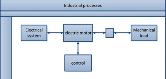
(18) II. DATA ANALYSIS. K Sτ. Detecting operating conditions and faults can be based on data analysis of various types of measurements (Fig. 1). The feedback information comes from performance indices. Nonlinear scaling brings all these to the same scale as numeric values and linguistic meanings.. p. Mα. p.  1 =  KS. ∑ [( KS. i =1. τ. p. M α )i. ]. 1/ p p. 1/ p.   .  1 =  KS.  ( M α )i  ∑ i =1  KS. τ. p. 1/ p. ,. (2). where Ks is the number of samples. Each sample has N variable values. As the aggregation can be continued to longer and longer time periods, this generalizes the practice used automation systems for the arithmetic means. High order derivatives of the acceleration signal improve fault detection [2, 3]. Stress analysis can be done without derivation, but the sensitivity is improved when higher orders α are used. Spectral norms also answer the question of which frequency range the changes are in since they combine the time domain analysis with the frequency domain analysis [24]. B. Performance indicators Harmonized indicators are used for monitoring maintenance actions on a management level, where the indicators are based on cost, time, man-hours, inventory value, work orders and cover of the criticality analysis [6, 7].. Fig.1. Detecting operating conditions and faults [23].. A. Features Normalisation or scaling of the data is needed since measurements with considerably different magnitudes cause problems in modelling. The nonlinear scaling extends modelling to various statistical distributions and allows recursive tuning. Arithmetic mean and standards deviation, which are the key statistical features in industrial practice, are special cases of generalized norms τ. M jp. p. = (τ M jp )1/ p = [(. 1 N. N. ∑ ( x ) )] i =1. p j i. 1/ p. ,. (1). where the order of the norm p ∈ ℜ is non-zero. The analysis is based on consecutive equally sized samples. Duration of each sample is called sample time, denoted τ, and N is the number values in the sample. For waveform signals, the number of signal values N = τ N s , where N s is the number of signal values which are taken in a second. The norm (1) has the same dimensions as the signals x (α ) , where α is the order of j. derivation, e.g. α =2 for widely used acceleration signals. The analysis can also use derivated signals. The generalized norms were introduced for condition monitoring [2, 3]. The norm values increase monotonously with increasing order if all the signals are not equal. The computation of the norms can be divided into the computation of equal sized sub-blocks, i.e. the norm for several samples can be obtained as the norm for the norms of individual samples. The same result is obtained using the norms of the sub-blocks:. ISBN 978-91-7583-841-0. Key performance indicators (KPIs) are quantifiable measures which reflect the critical success factors and the goals of the organization. KPIs differ depending on the organization and can focus on different parts and levels of the process. Accurately defined and measured KPIs provide feedback information for decision making. The maintenance function covers various aspects, including quality assurance, financial, reliability, planning, execution, strategic, data completeness, logistics and competency [9]. The performance metrics can be assessed with the SMART criteria: specific, measurable, attainable, realistic and timely [8]. Overall equipment effectiveness (OEE) is a set of broadly accepted non-financial metrics which reflects the manufacturing success by availability (uptime), performance rate and quality rate [10, 11]. C. Nonlinear scaling The z-score based linear scaling solutions are extended to asymmetric nonlinear scaling functions f defined by two second order polynomials (Fig. 2). The parameters of the polynomials are defined with five parameters corresponding the operating point c j and four corner points of the feasible range [25]. The feasible range is defined as a trapezoidal membership function defined by support and core areas, see [26]. The scaling functions are monotonously increasing throughout the feasible range, see [22, 27]. This is satisfied if the coefficients, a −j. =. a +j. =. (cl ) j − min( x j ) c j − (cl ) j max( x j ) − (ch ) j ( ch ) j − c j. 1. = =. (cl ) j − min( x j ) ∆c −j , max( x j ) − (ch ) j. (3). ∆c +j. . are restricted to the range  , 3 . 3 . 4.

(19) The scaled values are obtained by means of the inverse −1 function f : 2 with x j ≥ max( x j )   + +2 +  − b j + b j − 4 a j (c j − x j ) c j ≤ x j ≤ max( x j ) (4) − 2 with  2a +j  Xj = − −2 −  − b j + b j − 4 a j (c j − x j ) min( x j ) ≤ x j ≤ c j − 2 with  2a j  − 2 with x j ≤ min( x j ) . where. a −j , b −j , a +j. and. (LE) modelling since the indices are dimensionless. Grouping is important for large scale systems [28]. The cavitation index is an example of a stress index [4]: the approach provides four levels whose values ranges shown in TABLE I are consistent with the limits of the vibration severity ranges defined in [29, 30]. Strong cavitation can be avoided with better allocation of the energy production [31]. In a hot rolling mill, the stress indices were developed by using torque measurements: the feature is difference between the effective and average values, i.e.. xT = [(. b +j are coefficients of the. corresponding polynomials represented by 1 a −j = (1 − a −j ) ∆c −j , 2 1 − b j = (3 − a −j ) ∆c −j , 2 1 + a j = (a +j − 1) ∆c +j , 2 1 + b j = (3 − a +j ) ∆c +j . 2. N. ∑ ( x j )i2 )]. 1/ 2. i =1. −. 1 N. N. ∑ (x ) , i =1. (6). j i. where x j is the fillet split. The time interval can be different (5). Data-based tuning by using generalized norms and skewness was introduced in [4]. The constraints are taken into account by moving the corner points or the upper and lower limits if needed. The systems can be tuned with genetic algorithms [27].. for the passes. Since the orders of the norm are here 1 and 2, also negative values of x j can be used [32]. Stress indices for the front axle of a load haul dumper (LHD) have been developed from acceleration signals by using 5 4 feature max( M 2 ) . The analysis provides good indications of different stress contributions in these machines, which operate in harsh conditions where failures may be difficult to repair [33]. The cumulative stress method has recently been used in the monitoring of a rod mill [34], [35]. TABLE I. SEVERITY OF CAVITATION [4] Level. Fig.2. Feasible shapes of membership definitions fj and corresponding derivatives Dj: coefficients adjusted with the core (left) and support (right). Derivatives are presented in three groups: (1) decreasing and increasing, (2) asymmetric linear, and (3) increasing and decreasing [27].. D. Intelligent indices Intelligent indices are obtained from measurements and features by the nonlinear scaling approach. The indices obtained from short samples are aimed for use in the same way as indirect measurements, e.g. to indicate stress or condition (Fig. 1). Several indices can be combined in linguistic equation. Severity classification Cavitation index ( 4) C. < −1. 1. I. 2. −1 ≤ I. 3. 0 ≤ I C( 4 ) < 1. 4. ISBN 978-91-7583-841-0. 1 N. I. ( 4) C. ( 4) C. ≥1. <0. Cavitation level. Cavitation-free Short periods of weak cavitation Short periods of cavitation Cavitation. Severity. Good Usable Still acceptable Not acceptable. Intelligent indices based on two generalized norms are highly sensitive to faulty situations in the supporting rolls of a lime kiln. Surface damage and misalignment are clearly detected. The data set covers surface problems, good conditions after grinding, misalignment, stronger misalignment, very good conditions after repair work, and very good conditions one year later [4]. Sensitivity is also improved for weak friction and small fluctuations. This is useful in detecting lubrication problems. All the supporting rolls can be analyzed using the same approach throughout the data set. The results are consistent with the vibration severity criteria: good, usable, still acceptable, and not acceptable. The condition indices of the LHD machine need to be obtained repeatedly in similar steady operating conditions [33]. Extensions to real and complex order derivatives are discussed in [36].. 5.

(20) III. TEMPORAL ANALYSIS Fluctuations, trends and models are used in temporal analysis for all types of measurements, features and indices. Recursive updates of the parameters are needed in prognostics. A. Fluctuations The fluctuations are evaluated as the difference of the high and the low values as a difference of two moving generalized norms:. ∆x Fj (k ) =. K sτ. M jpH. pH. −. K sτ. M jpL. pL. ,. (7). I Dj (k ) =. (. ). 1 X j (k ) + I Tj (k ) + DI Tj (k ) , 3. (9). whose absolute values are highest when the difference to the set point is very large and is getting still larger with a fast increasing speed. The trend analysis is tuned to applications by selecting variable specific the time periods (n L ) j and (n S ) j . The thresholds. ε 1− = ε 1+ = ε 2− = ε 2+ = 0.5 .. Further fine-tuning. can be done by adjusting the weight factors wTj 1 and wTj 2 used. where the orders pH ∈ ℜ and pL ∈ ℜ are large positive and negative, respectively. The norms are calculated from the latest F K +1 values, and an average of several latest values of ∆x j (k ) s. for the indices I Tj (k ) and ∆I Tj (k ) . The calculations are done with numerical values and the results are represented in natural language [39].. is used as the feature of fluctuation. The feature, which was originally developed for control [37], is easy to calculate and more robust than using the difference of the actual maximum and minimum. The fluctuation indices are calculated from features (7) by the nonlinear scaling. Similar calculations can be done for intelligent indices if the variations close to the normal conditions are important. B. Trend analysis For any variable x j , a trend index I Tj (k ) is calculated from the scaled values X j with k k  1  1 I Tj (k ) = w j  X j (k ) − X j (k ) , ∑ ∑ (nL ) j + 1 i = k − ( n L ) j  (nS ) j + 1 i = k − ( nS ) j . (8). which is based on the means obtained for a short and a long time period, defined by delays (n S ) j and (n L ) j , respectively. The weight w j is variable specific. The index value is in the linguistic range [-2, 2] representing the strength of both the decrease and increase of the variable x j . [38] Episode alternatives are shown in Fig. 3. An increase is detected if the trend index exceed a threshold I Tj (k ) > ε 1+ . Correspondingly, I Tj (k ) < ε 1− for a decrease. The derivative of the index I Tj (k ) , denoted as ∆I Tj (k ) , extends the analysis to nonlinear episodes. Trends are linear if the derivative is close to zero: ε 2− < ∆I Tj (k ) < ε 2+ . The concave upward monotonic increase (D) and the concave downward monotonic decrease (B) are dangerous situations, which introduce warnings and alarms. The concave downward monotonic increase (A) and the concave upward monotonic decrease (C) mean that a harmful trend is stopping.. Fig.3. Intelligent trend analysis [38].. Trend indices can be calculated from the scaled values of measurements and features, intelligent indices and linguistic information. Interpretation in natural language follows the same guidelines. C. Prognostics In a load haul dumper (LHD), the cumulative stress increases fast during the high stress periods and increase is practically stopped when the stress is low since only stress indices are taken into account in the cumulative stress. [33] Recursive updates of the scaling functions become important in prognostics since the machine or process device is in good condition in the starting point. The rough early estimates are gradually refined if the failure predictions are not yet real. The interaction models are not changed [40].. Severity of the situation can be evaluated by a deviation index. ISBN 978-91-7583-841-0. 6.

(21) D. Risk analysis Varying operating conditions have been taken into account in fatigue analysis [32, 41] by representing the Wöhler curves with a linguistic equation (10). I S = log10 ( N C ),. where the stress index is the scaled value of stress, I S = f −1 ( Si ) = f −1 ( τ M αp ) .. (11). The scaling of the logarithmic values of the number of cycles, N C (k ) , is linear. In each sample time, τ , the cycles N C (k ) are obtained by (10) and added to the previous contributions by C (k ) = C (k − 1) +. τ N C (k ). ,. (12). where the value range of the sum C is scaled to provide the fatigue risk in percents (%). The high stress contributions dominate in the summation. Correspondingly, the very low stress periods have a negligible effect, which is consistent with the idea of infinite lifetime. The summation of the contributions also reveals repeated loading and unloading, and the individual contributions provide indications for the severity of the effect. The stress levels can be followed by a generalized statistical process control approach [42]. At the risk level higher than 60%, a single high torque level can have a strong effect on the activation of a failure. IV. UNCERTAINTY PROCESSING Scaling functions developed in data analysis are the basis of the uncertainty processing. All scaled values and fuzzy terms can be interpreted in natural language. The fuzzy interface is also used to introduce additional expert knowledge in the calculations.. B. Knowledge-based information Domain expertise can include information about levels which can be translated into fuzzy numbers. The labels {very low, low, normal, high, very high} or {fast decrease, decrease, constant, increase, fast increase} can be represented by number {-2, -1, 0, 1, 2}. Different shapes of membership definitions result different sets of default membership functions: the locations depend on the core, the support and the centre point. However, the linguistic data can be understood as scaled values, whose membership functions are equally spaced, i.e. {2, -1, 0, 1, 2}. The overlap between adjacent linguistic terms expresses a smooth transition from one term to the other. [43] The fuzzy sets can be modified by fuzzy modifiers, which are used as intensifying adverbs (very, extremely) or weakening adverbs (more or less, roughly). The resulting terms, e.g. extremely A ⊆ very A ⊆ A ⊆ more or less A ⊆ roughly A, (1). correspond to the powers {4, 2, 1, ½, ¼} of the membership in the powering modifiers. The vocabulary can also be chosen in a different way, e.g. highly, fairly, quite [43]. Only the sequence of the labels is important. Linguistic variables can be processed with the conjunction (AND), disjunction (OR) and negation (NOT). More examples can be found in [44]. C. Fuzzy calculus Fuzzy calculus is suitable for processing fuzzy inputs and outputs in the rule-based fuzzy set systems, but the rule-based system is not necessarily needed (Fig. 4). The extension principle is the basic generalisation of the arithmetic operations if the inductive mapping is a monotonously increasing function of the input. The interval arithmetic presented by Moore [45] is used together with the extension principle on several membership α-cuts of the fuzzy number x j for evaluating fuzzy expressions [46-48]. Fuzzy inequalities produce new facts like A ≤ B and A = B for fuzzy inputs A and B.. A. Varying operating conditions The features and indices are calculated with problemspecific sample times and the variation with time is handled as uncertainty by presenting the indices as time-varying fuzzy numbers. The classification limits can also be considered fuzzy. The parameters of the scaling functions are specific to operating conditions, some changes can be taken into account switching the parameter sets. The parameters become fuzzy numbers if the time period includes different operating conditions. The results of the fuzzy scaling are fuzzy numbers for crisp values as well. All intelligent indices, including fluctuation, trend and deviation indices, can be presented as fuzzy numbers.. ISBN 978-91-7583-841-0. 7.

(22) Fig. 4. Combined fuzzy set system [22].. D. Fuzzy rule-based solutions In the combined systems, the fuzzy inputs can be fuzzy numbers or crisp inputs processed by fuzzy scaling functions (Fig. 4). The results can be defuzzified to crisp values, processed with fuzzy arithmetics or passed to other fuzzy set systems. Type-2 fuzzy models introduced by Zadeh in 1975 take into account uncertainty about the membership function [49]. Most systems based on interval type-2 fuzzy sets are reduced to an interval-valued type-1 fuzzy set. Special cases of fuzzy linguistic equation models, which can be understood as linguistic Takagi-Sugeno (LTS) type fuzzy models, are robust solutions for applications where the same variables can be used for defining operating areas and in the submodels. No special smoothing algorithms are needed [50]. V. OPERATION AND MAINTENANCE MANAGEMENT The nonlinear scaling approach is the basis of the consistent natural language interface. A. Monitoring and control The keys of the natural language interface are the monotonously increasing, nonlinear scaling functions, which are obtained by generalized norms and moments or defined manually based on domain expertise. The variable specific parameters can be recursively updated by using the corresponding norms and new data samples. Also the orders of the norms can be updated after drastic changes. Since the parameters specific to operating conditions, some changes can be taken into account switching the parameter sets. Uncertainty, fluctuations and confidence in results are estimated by a difference of norms of high positive and negative order, respectively. [39] Feature levels, uncertainty, trends, trend episodes and severity can be evaluated by using scaled values, fluctuation, trend indices and derivatives of trend indices (TABLE II). TABLE II.. MONITORING INTERFACE [39] Features / indices. Task Level. Scaled value. Variation / Fluctuation. Trend index. Derivative of trend index. x. Uncertainty. x. Trend. x. Trend episodes. x. x. x. x. Trend severity. x. All indices are in the range [-2, 2] and interpreted in natural language labels, e.g. {very low, low, normal, high, very high}. The trend index I Tj (k ) ) represents levels {fast decrease, decrease, constant, increase, fast increase}, the derivative ∆I Tj (k ) levels {fast accelerating decrease, accelerating. ISBN 978-91-7583-841-0. decrease, constant change, accelerating increase, fast accelerating increase} and the deviation index I Dj (k ) {serious decrease, decrease, normal, increase, serious increase}, respectively. The fuzzy partition of all these can be refined by using more levels. Advanced signal processing and feature extraction is combined with nonlinear scaling to obtain condition and stress indices in [33]. More information can be collected with reliability-centered maintenance (RCM) [5], and finally, all this can be monitored with statistical process control (SPC) [40]. Increased computational power in small programmable controllers and sensors open new possibilities for the efficient on-site calculations. Programmable automation controllers (PACs) make the algorithm testing efficient since the software can be updated easily and measurement setup can be customized. Several aspects connected to on-site calculations present a method for extracting meaningful numbers from high frequency vibration data [51, 52]. The monitoring interface is aimed to utilize on-line measurements in stabilizing, optimizing and coordinating control. B. Control strategies and Maintenance Process control systems in industry include centralized or decentralized process controllers coupled with hosts, workstations and several process control and instrumentation devices, such as field devices. Applications are related to business functions in Enterprise resource planning (ERP) or maintenance functions in computerized maintenance management systems (CMMS). Smart field devices can include equipment monitoring applications which are used to help monitor and maintain the devices. [23] Maintenance information is collected from various sources: condition monitoring measurements, performance indicators, including harmonized indicators, key performance indicators and overall equipment effectiveness (OEE). The systems include a huge amount of event information, which is not necessarily in a numeric form. The natural language information can be understood in the range [-2, 2] through linguistic levels and modifiers related [42]. At this level, the temporal analysis and uncertainty processing become important in detecting operating conditions. Model-based predictions and recursive updates of the parameters are needed in decision making, where the adaption of the control strategies is used in scheduling the conditionbased maintenance actions. C. Management Performance indicators are specific for different industrial areas [8], [12]. The nonlinear scaling brings the performance levels to a consistent range, which can be understood in linguistic terms. The levels and their improvements are represented in natural language, e.g. ’excellent improvement from poor performance to good performance’ [5]. Aggregation is needed for the information obtained from other levels. Uncertainty processing is increasingly important in this level.. 8.

(23) VI. CONCLUSIONS The nonlinear scaling approach is the main part of the data processing chain which is the integrating part of the natural language interface. The calculations are done in numeric forms, but the levels and all the indices based on them can be represented in natural language. The system includes integrated temporal analysis and uncertainty processing which facilitates the efficient use of domain expertise. ACKNOWLEDGMENT The author would like to thank the research program “Measurement, Monitoring and Environmental Efficiency Assesment (MMEA)” funded by the TEKES (the Finnish Funding Agency for Technology and Innovation) and the Artemis Innovation Pilot project “Production and energy system automation and Intelligent-Built (Arrowhead)”. REFERENCES [1]. [2]. [3]. [4]. [5]. [6]. [7] [8]. [9] [10] [11]. [12] [13]. [14]. S. Lahdelma, and E. Juuso, ”Advanced signal processing and fault diagnosis in condition monitoring,” Insight, vol. 49, no. 12, pp. 719-725, 2007, doi: 10.1784/insi.2007.49.12.719. S. Lahdelma, and E. Juuso, “Signal processing and feature extraction by using real order derivatives and generalised norms. Part 1: Methodology,” The International Journal of Condition Monitoring, vol. 1, no. 2, pp. 46-53, 2011, doi: 10.1784/204764211798303805. S. Lahdelma, and E. Juuso, “Signal processing and feature extraction by using real order derivatives and generalised norms. Part 2: Applications,” The International Journal of Condition Monitoring, vol. 1, no. 2, pp. 54-66, 2011, doi: 10.1784/204764211798303814. E Juuso and S Lahdelma, “Intelligent scaling of features in fault diagnosis,” 7th International Conference on Condition Monitoring and Machinery Failure Prevention Technologies, CM 2010 – MFPT 2010, 7th International Conference on Condition Monitoring and Machinery Failure Prevention Technologies, Stratford-upon-Avon, UK. BINDT, vol. 2, pp. 1358-1372, June 2010. E. K. Juuso, and S. Lahdelma, “Intelligent performance measures for condition-based maintenance,” Journal of Quality in Maintenance Engineering, vol. 19, no.3, pp. 278-294, 2013, doi: 10.1108/JQME-052013-0026. C. Olsson, and T. Svantesson, “Harmonised maintenance and reliability indicators – compare apples to apples,” Maintworld, vol. 1, no. 1, 2009, pp. 9-11. C. Idhammar, “The first world class maintenance organization,” Maintworld, vol. 2, no. 2, pp. 52-53, 2010. A. Parida, and U. Kumar, “Maintenance performance measurement – methods, tools and applications,” Maintworld, vol. 1, no. 1, pp. 30-33, 2009. N. A. Al-Shammasi, and S. S. Al-Shakhoyry, “Improving maintenance performance in Saudi Aramco,” Maintworld, vol. 2, no. 2, pp. 6-9, 2010. SCEMM Keep It Running – Industrial Asset Management, Painoyhtymä, Loviisa, 1998. B. Hägg, “Maintenance – an investment in higher profitability,” Maintenance, Condition Monitoring and Diagnostics 2010, Proceedings of the International Conference in Oulu, POHTO Publications, Oulu, 2930 September, pp. 7-14, 2010. P. Willmott, “Post the streamlining – ‘where’s your maintenance strategy now?” Maintworld, vol. 2, no. 1, pp. 16-22, 2010. S. Dash, R, Rengaswamy, and V. Venkatasubramanian, “Fuzzy-logic based trend classification for fault diagnosis of chemical processes,” Computers and Chemical Engineering, vol. 27, pp. 347–362, 2003. J. T.-Y. Cheung, and G. Stephanopoulos, “Representation of process trends - part I. A formal representation framework,” Computers & Chemical Engineering, vol. 14, no. 4/5, pp. 495–510, 1990.. ISBN 978-91-7583-841-0. [15] A. K. S. Jardine, D. Lin, and D. Banjevic, “A review on machinery diagnostics and prognostics implementing condition-based maintenance,” Mechanical Systems and Signal Processing, vol. 20, no, 7, pp. 1483–1510, 2006, doi: 10.1016/j.ymssp.2005.09.012. [16] A. H. Christer, and W. Wang, “A model of condition monitoring inspection of production plant,” International Journal of Production Research, vol. 30, no. 9, pp. 2199-2211, 1992. [17] W. Wang, “A two-stage prognosis model in condition based maintenance,” European Journal of Operational Research, vol. 182, no. 3, pp. 1177-1187, 2007. [18] W. Schütz, W. “A history of fatigue, Engineering Fracture Mechanics,“ vol. 54, no. 2, pp. 263-300, 1996. [19] A. Palmgren, “Die Lebensdauer von Kugellagern,” Verfahrenstechnik, vol. 68, pp. 339-341, 1924. [20] M. A. Miner, “Cumulative damage in fatigue,” ASME Journal of Applied Mechanics, vol. 67, pp. 159-164, 1945. [21] L. A. Zadeh, “Fuzzy sets,” Information and Control, vol. 8, pp. 338–353, 1965. [22] E. K. Juuso, “Intelligent Methods in Modelling and Simulation of Complex Systems,” Simulation Notes Europe SNE, vol. 24, no. 1, pp. 110. Selected SIMS 2013, 2014, doi: 10.11128/sne.24.on.102221. [23] E. K. Juuso and D. Galar, ”Intelligent real-time risk analysis for machines and process devices,” Current Trends in Reliability, Availability, Maintainability and Safety: An Industry Perspective, Lecture Notes in Mechanical Engineering, Springer, pp. 229-240, 2016, doi: 10.1007/978-3-319-23597-4_17. [24] K. Karioja, and E. Juuso, “Generalised spectral norms – a new method for condition monitoring,” International Journal of Condition Monitoring, vol. 6, no. 1, pp. 13-16, 2016 March, doi: 10.1784/204764216819257150. [25] E. K. Juuso, “Integration of intelligent systems in development of smart adaptive systems,” International Journal of Approximate Reasoning, Vol. 35, no. 3, pp. 307–337, 2004, doi: 10.1016/j.ijar.2003.08.008. [26] H. J. Zimmermann, Fuzzy set theory and its applications, Kluwer Academic Publishers, 1992. [27] E. K. Juuso, “Tuning of large-scale linguistic equation (LE) models with genetic algorithms,” Adaptive and Natural Computing Algorithms, Revised selected papers - ICANNGA 2009, Kuopio, Finland ICANNGA 2009, Lecture Notes in Computer Science (LNCS) 5495, pp 161-170, Springer, Heidelberg, 2009, doi: 10.1007/978-3-642-04921-7_17. [28] T. Ahola, E. Juuso, and K. Leiviskä, “Variable Selection and Grouping in a Paper Machine Application,” International Journal of Computers, Communications & Control, vol. II, no. 2, pp. 111-120, 2007. [29] VDI 2056 Beurteilungsmaβstäbe für mechanische Schwingungen von Maschinen, VDI-Richtlinien, Oktober 1964. [30] R. A. Collacott, Mechanical Fault Diagnosis and condition monitoring, Chapman and Hall, London, 1977. [31] E. Juuso and S. Lahdelma, “Cavitation Indices in Power Control of Kaplan Water Turbines,” 6th International Conference on Condition Monitoring and Machinery Failure Prevention Technologies, CM 2009 – MFPT 2009, Dublin, Ireland. BINDT, vol. 2, pp. 830-841, June 2009. [32] E. Juuso, and M. Ruusunen, ”Fatigue prediction with intelligent stress indices based on torque measurements in a rolling mill,” 10th International Conference on Condition Monitoring and Machinery Failure Prevention Technologies, CM 2013 - MFPT 2013, 18-20 June 2013, Krakow, Poland, vol. 1, pp. 460-471. [33] E. K. Juuso, “Intelligent indices for online monitoring of stress and condition,” 11th International Conference on Condition Monitoring and Machinery Failure Prevention Technologies, CM 2014/MFPT 2014, Manchester, UK, 10-12 June, vol. 1, 2014, pp. 637-648. [34] J. Laurila, A. Koistinen, E. Juuso, and T. Liedes, ”Monitoring of a rod mill using advanced feature extraction methods,” 12th International Conference on Condition Monitoring and Machinery Failure Prevention Technologies, CM2015/MFPT2015, Oxford, United Kingdom 9-11 June 2015, pp. 580-590. [35] A. Koistinen, J. Laurila, and E. Juuso, ”Rod mill liner monitoring using cumulative stress,” 13th International Conference on Condition. 9.

(24) [36]. [37]. [38]. [39]. [40]. [41]. [42]. [43]. Monitoring and Machinery Failure Prevention Technologies, CM2016/MFPT2016, Paris, France 10-12 October 2016, pp. 131-142. J. Nissilä, S. Lahdelma, and J. Laurila, “Condition monitoring of the front axle of a load haul dumper with real order derivatives and generalised norms,” 11th International Conference on Condition Monitoring and Machinery Failure Prevention Technologies, CM 2014/MFPT 2014, Manchester, UK, 10-12 June, Vol. 1, 2014, pp. 407426. E. K. Juuso, “Model-based adaptation of intelligent controllers of solar collector fields,” 7th Vienna Symposium on Mathematical Modelling, February 14-17, 2012, Vienna, Austria, Part 1, IFAC, 2012, vol. 7, pp. 979–984, doi: 10.3182/20120215-3-AT-3016.00173. E. K. Juuso, “Intelligent Trend Indices in Detecting Changes of Operating Conditions,” 2011 UKSim 13th International Conference on Computer Modelling and Simulation (UKSim), IEEE Computer Society, 2011, pp. 162-167, doi: 10.1109/UKSIM.2011.39. E. K. Juuso, “Informative process monitoring with a natural language interface,” 2016 UKSim-AMSS 18th International Conference on Modelling and Simulation, IEEE Computer Society, 2016, pp. 105-110, doi: 10.1109/UKSim.2016.37. E. K. Juuso, “Recursive Data Analysis and Modelling in Prognostics,” 12th International Conference on Condition Monitoring and Machinery Failure Prevention Technologies, 9-12 June 2015, Oxford, UK. NY, USA: Curran Associates, 2015, pp. 560-567. E. K. Juuso and M. Ruusunen, ”Stress Indices in Fatigue Prediction,” Maintenance, Condition Monitoring and Diagnostics & Maintenance Performance Measurement and Management - MCMD 2015 and MPMM 2015, 30th September - 1st October, 2015, Oulu, Finland. Oulu: Pohto. E. K. Juuso, ”Generalised statistical process control (GSPC) in stress monitoring,” IFAC-Papers OnLine, vol. 28, no. 17, pp. 207-212, 2015, doi: 10.1016/j.ifacol.2015.10.104. E. K. Juuso, “Integration of knowledge-based information in intelligent condition monitoring,” 9th International Conference on Condition. [44] [45] [46] [47]. [48]. [49] [50]. [51]. [52]. Monitoring and Machinery Failure Prevention Technologies, 12-14 June 2012, London, UK. NY, USA: Curran Associates, 2012, vol. 1, pp. 217– 228. M. De Cock and E. E. Kerre, “Fuzzy modifiers based on fuzzy relations,” Information Sciences, vol. 160, no. 1-4, pp. 173–199, 2004. R. E. Moore, Interval Analysis. Englewood Cliffs, NJ:Prentice Hall. 1966. J. J. Buckley, and T. Feuring, “Universal approximators for fuzzy functions,” Fuzzy Sets and Systems, vol. 113, pp. 411–415, 2000. J. J. Buckley, and Y. Hayashi, “Can neural nets be universal approximators for fuzzy functions?” Fuzzy Sets and Systems, vol. 101: 323–330, 1999. J. J. Buckley, and Y. Qu, “On using α-cuts to evaluate fuzzy equations,” Fuzzy Sets and System, vol. 38, no. 3, pp. 309–312, 1990, doi: 10.1016/0165-0114(90)90204-J J. M. Mendel, “Advances in type-2 fuzzy sets and systems,” Information Sciences, vol. 177, no. 1, pp. 84–110, 2007. E. K. Juuso, “Development of Multiple Linguistic Equation Models with Takagi-Sugeno Type Fuzzy Models,” 2009 International Fuzzy Systems Association WORLD CONGRESS & 2009 European Society for Fuzzy Logic and Technology CONFERENCE, IFSA-EUSFLAT 2009, 20-24 July 2009, Lisbon, Portugal, pp. 1779-1784. A. Koistinen, and E. K. Juuso, ”On-site calculations of generalised norms for maintenance and operational monitoring,” Maintenance, Condition Monitoring and Diagnostics & Maintenance Performance Measurement and Management - MCMD 2015 and MPMM 2015, 30th September - 1st October, 2015, Oulu, Finland. Oulu: Pohto. A. Koistinen, and E. K. Juuso, ”Information from Centralized Database to Support Local Calculations in Condition Monitoring,” 9th EUROSIM Congress on Modelling and Simulation, 12-16 September 2016 in Oulu, Finland. IEEE Computer Society, pp. 1049-1054. doi: 10.1109/EUROSIM.2016.86. .. ISBN 978-91-7583-841-0. 10.

(25) Appendix: Intelligent performance analysis with a natural language interface. ISBN 978-91-7583-841-0. 11.

(26) ISBN 978-91-7583-841-0. 12.

(27) ISBN 978-91-7583-841-0. 13.

(28) ISBN 978-91-7583-841-0. 14.

(29) ISBN 978-91-7583-841-0. 15.

(30) ISBN 978-91-7583-841-0. 16.

(31) ISBN 978-91-7583-841-0. 17.

(32) ISBN 978-91-7583-841-0. 18.

(33) ISBN 978-91-7583-841-0. 19.

(34) ISBN 978-91-7583-841-0. 20.

(35) ISBN 978-91-7583-841-0. 21.

(36) ISBN 978-91-7583-841-0. 22.

(37) ISBN 978-91-7583-841-0. 23.

(38) ISBN 978-91-7583-841-0. 24.

(39) ISBN 978-91-7583-841-0. 25.

(40) Bayesian Networks in Fault Diagnosis: Some research issues and challenges Baoping Cai1*, Lei Huang2, Jing Lin3, Min Xie4 caibaoping@upc.edu.cn; 2huanglei1@s.upc.edu.cn; 3janet.lin@ltu.se; 4minxie@cityu.edu.hk 1, 2 College of Mechanical and Electronic Engineering, China University of Petroleum, Qingdao, Shandong 266580, China 3 Department of Civil, Environmental and Natural Resources Engineering, Operation, Maintenance and Acoustics, Luleå University of Technology, Luleå, Sweden 1, 4 Department of Systems Engineering and Engineering Management, City University of Hong Kong, Kowloon, Hong Kong 1. Abstract—Fault diagnosis is useful in helping technicians detect, isolate, and identify faults, and troubleshoot. Bayesian network (BN) is probabilistic graphical model that effectively deals with various uncertainty problems. This model is increasingly utilized in fault diagnosis. This paper presents bibliographical review on use of BNs in fault diagnosis in the last decades with focus on engineering systems. This work also presents general procedure of fault diagnosis modeling with BNs; processes include BN structure modeling, BN parameter modeling, BN inference, fault identification, validation, and verification. The paper provides series of classification schemes for BNs for fault diagnosis, BNs combined with other techniques, and domain of fault diagnosis with BN. This study finally explores current gaps and challenges and several directions for future research. Index Terms—Bayesian networks, fault diagnosis. I.. INTRODUCTION. W. ITH rapid development of modern industrial systems, systematic complexity increases constantly. Therefore, fault diagnosis must be utilized to obtain high reliability and availability. Fault diagnosis quickly detects process abnormality and component fault and identifies root causes of these failures by using appropriate models, algorithms, and system observations. Therefore, fault diagnosis system is useful in assisting operations staff to detect, isolate, and identify faults and to aid in troubleshooting. In general, fault diagnosis approaches can be classified into three categories: model-based [1], signal-based [2], and data-driven approaches [3]. In model-based approach, focus is on establishing mathematical models of complex industrial systems. These models can be constructed by various identification methods, physical principles, etc. Signal-based approach uses detected signals to diagnose possible abnormalities and faults by comparing detected signals with prior information of normal industrial systems [4]. Usually, difficulty occurs in building accurate mathematical models and obtaining accurate signal patterns for complex industrial and process systems. Data-driven fault diagnosis approach requires large amount of historical data, rather than models or signal patterns [5]. Therefore, data-driven methods are suitable for complex industrial systems. Data-driven fault diagnosis approach is also called knowledge-based fault diagnosis approach. Knowledge information can be obtained based on either statistical or ISBN 978-91-7583-841-0. non-statistical approach. Data-driven approach can be categorized into statistics-based and non-statistics-based fault diagnosis approaches [5]. The former includes principal component analysis [6], independent component analysis [7], and support vector machine [8], whereas the latter includes neural network [9], fuzzy logic [10], etc. BN is an important probabilistic graphical model, which can deal effectively with various uncertainty problems based on probabilistic information representation and inference. As representational tool, BN is quite attractive for three reasons. First, BN is consistent and complete represents and defines unique probability distribution over network variables. Second, the network is modular; its consistency and completeness are ensured using localized tests, which are only applicable to variables and their direct causes. Third, BN is compact representation, as it allows specification of exponentially sized probability distribution using polynomial of probabilities [11]. Hence, this tool is deeply researched and widely used in many domains ranging from reliability engineering [12–14], risk analysis [15], and safety engineering [16] to resilience engineering [17]. During the last decades, BNs are studied and utilized in domain of fault diagnosis, which is typically data-driven approach. BN-based fault diagnosis models are established using huge amount of historical data. Diagnosis is conducted by backward analysis with various algorithms [18]. That is, we input observed information into evidence nodes, update posterior probabilities of fault nodes based on BN inference, and identify root causes of failure using identification rules. Research attracted considerable attention, solved some important problems of BN-based fault diagnosis, and focused on challenging problems. A large number of literatures, including theory research and project application, were about conference proceedings and technical reports. To our knowledge, literature never reviewed use of BNs in fault diagnosis. This paper aims to review latest research results of BNbased fault diagnosis approaches to provide reference and to identify future research directions for fault diagnosis researchers and engineers. The remainder of the paper is organized as follows. Section II presents general procedures of fault diagnosis with BNs. Section III introduces types of BNs for fault diagnosis; these types include BNs, dynamic Bayesian networks (DBNs) and object-oriented Bayesian networks (OOBNs). Section IV identifies few on-going and upcoming research directions. Section V summarizes this paper.. 26.

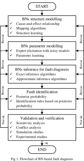
(41) II.. PROCEDURES OF FAULT DIAGNOSIS WITH BNS. Fault diagnosis procedures with BNs consist of BN structure modeling, BNs parameter modeling, BN inference, fault identification, and validation and verification. Figure 1 provides detailed flowchart of the process. START. Cause-and-effect relationship Mapping algorithms Structure learning.  . Expert elicitation with noisy models Parameter learning. Revise. Revise. BNs structure modelling   . Exact inference algorithms Approximate inference algorithms.  . Posterior probability Identification rules based on posterior probability.    . Sensitivity analysis Conflict analysis Simulation studies Experimental studies. Fault identification. alidation and verification. Revise Revise. BNs inference for fault diagnosis  . Not ok. Not ok. Revise. Revise. BNs parameter modelling. ok. END Fig 1. Flowchart of BN-based fault diagnosis. A.. BN structure modelling Several methods were reported in constructing BN structure models for fault diagnosis. Three main methods include cause-and-effect relationship, mapping algorithms, or structuring learning. Per cause-and-effect relationship method, one reflects on their knowledge and experience about faults and fault symptoms and then captures them into a BN. That is, network structure is established based on causal relationship between faults and fault symptoms. BN structure is usually composed of two layers of events: fault layer and fault symptom layer. For example, Dey and Stori [19] presented BN-based process monitor and fault diagnosis method for combining multi-sensor data during machining operation to diagnose root causes of process variations. Root layer and evidence layer consist of structure of proposed BNs for root cause diagnosis. Aside from two basic layers, other layers representing various information are added and established in BN structure to improve fault diagnostic performances. Cai et al. [20] developed BN-based ground-source heat pump fault diagnosis system by fusing multi-sensor data. A new layer, which is observed information layer, is established to connect to the fault layer directly for improving performance and increasing fault diagnosis accuracy.. ISBN 978-91-7583-841-0. Per mapping algorithms, one automatically synthesizes BN from other type of formal knowledge or models, such as fault tree and bow tie models. Lampis and Andrews [21] proposed a system fault diagnosis method by converting fault trees into BNs. These people built non-coherent fault tree model for fault diagnosis of systems and mapped it to BNs following a two-step rule. According to structure learning, BN structure can be constructed based on learning from data related to faults and fault symptoms when sufficient data are available. Given that learning is inductive process, principle of induction guides construction processes, such as maximum likelihood approach and Bayesian approach. Jin et al. [22] presented BN-based fault detection and diagnosis method of assembly fixture. These scientists proposed structure learning method by using mutual information test to obtain causal relationships among fixture and sensor nodes. Former two methods are sometimes known as knowledge representation methods, whereas the third one is known as machine learning method. Networks constructed by knowledge representation methods have different nature from those constructed by machine learning method. For example, former networks had larger sizes and placed harsher computational demands on reasoning algorithms. Moreover, these networks had significant amount of determinism (i.e., probabilities equal to 0 or 1), allowing them to benefit from computational techniques, which may be irrelevant to networks constructed by machine learning method [11]. However, the former two methods, especially cause-and-effect relationship method, may produce inaccurate models. Although structure learning method is more accurate, difficulty or impossibility sometimes arise from obtaining available and sufficient data for learning. Of course, simulation methods can be used to generate required data to fill this gap. B.. BN parameter modeling BNs parameter model consists of prior probability of root nodes and conditional probability of leaf nodes. Prior probabilities of events are calculated before acquisition of new evidence, observation or information. These data can be achieved from expert knowledge and experience and statistical results of historical, simulated, and experimental data. With increasing prior probability, events have higher probability of happening. In general, in fault diagnosis, we assume that prior probabilities of all fault nodes are identical to emphasize posterior probabilities with new observations [20]. Conditional probabilities expectedly take place when other events are known to occur. These probabilities are usually contained in conditional probability table (CPT). Various ways exist for obtaining CPTs generally fall into two main approaches: knowledge elicitation from experts and data-driven parameterization through machine learning methods. Knowledge elicitation from experts has disadvantages, including specificity of exponential growth of parameters. To specify complete CPT for child node m n with sm states and n parent nodes, ( sm − 1)∏ si i =1. probabilities should be evaluated; si is number of states of parent node i [23]. Suppose that we have variables with n parents, and that each variable has only two values. We then need 2n independent parameters to completely specify CPT for the variable. Modeling arises as number of parents, n,. 27.

(42) becomes larger. Noisy-OR and noisy-MAX models were reported to simplify knowledge elicitation from experts of CPTs. When a node is Boolean type and has normal and abnormal states, which can be detected by sensors, node CPT can be simplified with noisy-OR model. Supposing that all nodes are Boolean, several causes X1, X2, …, Xn lead to an effect Y, and CPT can be generated with only n parameters, and q1, q2, …, qn are obtained using the following: n. P (Y = 1| X 1 , X 2 ,..., X n ) = 1 − ∏ qi i =1. (1) where qi is probability for each parent with false Y when Xi is true, and all other parents are false [24]. Recently, Cai et al. utilized noisy-OR and noisy-MAX models to determine complete CPTs of BNs for fault diagnosis of complex industrial systems, such as groundsource heat pump [20] and subsea production systems [24]. Kraaijeveld and Druzdzel [25] proposed method to simplify and speed up design in constructing diagnostic BNs, and interaction among variables was modeled by noisy-MAX gates. Notably, knowledge elicitation from experts using noisy models may cause errors even in diagnostic results because of independent assumptions of these models. Noisy models are for local structures only. Each noisy model is based on assumptions about interactions of parents with their common child. When assumption corresponds to reality, then noisy models are used for local structure. Otherwise, resulting Bayesian network will be inaccurate model (but it could be a good approximation). CPTs are also generated through BN parameter learning from historical data. This method is similar to structure learning; its advantage includes more accurate BN parameter model, whereas its disadvantage is difficult and sometimes impossible acquisition of available and sufficient historical data. For instance, SIAM database was used for learning of CPTs of BN models for railway diagnosis [26]. C.. BN inference Based on conditional independence assumptions and chain rules, joint probability of variables U = {A1, A2, …, An} can be calculated as follows: n. P(U ) = ∏ P( Ai | Pa( Ai )) i =1. (2) where Pa(Ai) is parent node of Ai in BNs. BNs can perform backward or diagnostic analyses with various kind of inference algorithms based on Bayes’ theorem, which is as follows: [27] P( E | U ) P(U ) P ( E ,U ) P(U | E ) = = P( E ) ∑ U P ( E ,U ) (3) In general, inference algorithms are divided into exact inference and inferences. Exact inference algorithms can compute exact probabilities of variables and include message-passing, conditioning, junction tree, symbolic probabilistic inference, arc reversal/node reduction, and differential algorithms. Approximate inference computes approximate probabilities of variables with statistical approach. This inference includes algorithms for stochastic sampling, search-based algorithm, and loopy belief ISBN 978-91-7583-841-0. propagation algorithm. For complex BNs, inference is NP hard problem. Exact inference algorithms, for example, junction tree, were used in fault diagnosis of single-tank systems [28] and end-to-end service quality of qualitative diagnosis [29]. Complexity in exact inference algorithms leads to surge of interest in approximate inference algorithms, which are generally independent of treewidth. Today, approximate inference algorithms are the only choice for networks having large treewidth. Yet, such algorithms lack sufficient local structure. For example, Wiegerinck, et al. [30] adapted variational methods with tractable structures to develop approximate inference algorithm of BNs for medical diagnosis. D.. Fault identification Fault identification is conducted based on posterior probabilities of fault nodes based on provided evidence. Only probabilities of faults can be given, but definite diagnostic results cannot be drawn per posterior probabilities. Overall, corresponding fault has higher probability of occurrence with increasing posterior probability. For some fault diagnoses, diagnostic result is directly determined by posterior probability. For instance, in BNbased fault diagnosis systems for manufacturing tests of mobile telephone infrastructure, nodes with highest posterior probability of failure state were considered as either tokens to second BN or advice nodes. When nodes were the former, existing BN was saved as case, and other BNs defined in the token were loaded. In case of the latter, nodes were considered to be advice nodes [31]. In BN-based control loop diagnosis, according to maximum a posteriori principle, the mode with biggest posterior probability is potential fault mode, and abnormalities related to this fault mode were root causes of failure [32]. Notably, used algorithm may cause some errors when posterior probability is used directly for fault identification, because some faults have inherently high prior probability (before BN inference), or simultaneous faults may exist. Therefore, to increase accuracy and robustness of fault diagnosis, a series of fault identification rules were reported for determination of diagnostic results. In BN-based inverter fault diagnosis, the following identification methods are defined: (a) system reports a single open-circuit of switch with highest posterior probability when it is higher than 70%, or 50% higher than the second highest one; (b) system reports double opencircuit failure of switch with highest and second highest posterior probabilities when both are higher than 70% or 50 higher than the third highest one [33]. Remarkably, for different fault diagnosis systems, one should develop corresponding different fault identification rules. This goal requires complex work, because rules must be defined, tested, and revised repeatedly until achievement of satisfactory diagnostic performance. E.. Verification and Validation Model verification and validation are significant aspects of fault diagnosis because they provide reasonable confidence to diagnostic results. Many methods, such as sensitivity analysis, conflict analysis, simulation and experimental research, are used for BN-based fault diagnosis verification and validation. Specifically,. 28.

No results found