SKI Report 99:55
Research
Risk Based Test Interval and
Maintenance Optimisation
Application and Uses
Erik Sparre
October 1999
SKI Report 99:55
Research
Risk Based Test Interval and
Maintenance Optimisation
Application and Uses
Erik Sparre
RELCON AB
Box 1288
SE-172 25 Sundbyberg
Sweden
October 1999
This report concerns a study which has been conducted for the Swedish Nuclear Power Inspectorate (SKI). The conclusions and viewpoints presented in the report are
TABLE OF CONTENTS
Summary...5
Sammanfattning...6
Acronyms and Abbreviations ...7
1 Introduction...9
2 Purpose and Scope of the Project...9
3 Method ...10
3.1 Overview ...10
3.2 Assumptions and Limitations ...10
3.3 Procedure...11
4 Description of the PSA Model ...14
4.1 Overview ...14 4.2 Initiating Events...14 4.3 System Level ...15 5 Software ...15 6 Analyses ...15 6.1 Original Optimisation...16
6.2 Failure Data Uncertainties...19
6.3 Deterministic Uncertainties ...21
6.4 Plant Configuration ...23
6.5 Outage Times Caused By Test ...24
6.6 Calculation Technique...27 7 Summary of Results ...33 7.1 Discussion of Results ...35 8 Conclusions...37 9 References...38
APPENDICES
TABLES
Table 1: Original optimisation RiskSpectrum DOS...17
Table 2: Original optimisation RiskSpectrum PSA Professional ...17
Table 3: Example of how proportions between time dependent and time independent failure data is modified ...20
Table 4: Failure data 50% time dependent ...20
Table 5: Failure data 100% time dependent ...20
Table 6: Result of optimisation when feed water system is not included in the PSA model ...22
Table 7: Investigated plant configurations ...23
Table 8: Results of optimisations when analysing different plant configurations.23 Table 9: Result of optimisation with adjusted maintenance unavailability...26
Table 10: Parameters in example for calculation technique...28
Table 11: Results of calculations in example ...31
Table 12: Result of optimisation using time dependent calculations ...32
Table 13: Summary of optimisation results ...33
Table 14: Range of test intervals after optimisation...36
Table 15: Evaluation of two alternative test schemes ...37
DIAGRAMS
Diagram 1: Component unavailability ...25Diagram 2: Example of time dependent unavailabilities for P1 and P2 ...29
Diagram 3: Example staggered testing versus sequential testing ...30
Diagram 4: Results of optimisation (RiskSpectrum DOS) ...34
Summary
In this report the work conducted in the project “Risk Based Test Interval and
Maintenance Optimisation – Application and Uses” is described. The project is part of an IAEA co-ordinated Research Project (CRP) on “Development of Methodologies for Optimisation of Surveillance Testing and Maintenance of Safety Related Equipment at NPPs”.
The purpose of the project is to investigate the sensitivity of the results obtained when performing risk based optimisation of the technical specifications. Previous projects have shown that complete LPSA models can be created and that these models allow optimisation of technical specifications. However, these optimisations did not include any in depth check of the result sensitivity with regards to methods, model completeness etc.
Four different test intervals have been investigated in this study. Aside from an original, nominal, optimisation a set of sensitivity analyses has been performed and the results from these analyses have been compared to the original optimisation.
The analyses indicate that the result of an optimisation is rather stable. However, it is not possible to draw any certain conclusions without performing a number of sensitivity analyses. Significant differences in the optimisation result were discovered when
analysing an alternative configuration. Also deterministic uncertainties seem to affect the result of an optimisation largely.
The sensitivity of failure data uncertainties is important to investigate in detail since the methodology is based on the assumption that the unavailability of a component is dependent on the length of the test interval.
Sammanfattning
I denna rapport redovisas det arbete som har genomförts inom projektet “Risk Based Test Interval and Maintenance Optimisation – Application and Uses”. Projektet är en del i ett samordningsprojekt organiserat av IAEA, “Development of Methodologies for Optimisation of Surveillance Testing and Maintenance of Safety Related Equipment at NPPs”.
Syftet med projektet är att undersöka de resultatosäkerheter som uppkommer vid riskbaserad optimering av STF. Tidigare genomförda projekt har visat att det är möjligt att skapa kompletta LPSA modeller och att det är möjligt att genomföra en riskbaserad optimering av STF. Hittills har emellertid ingen djupare undersökning gjorts av de osäkerheter som finns i resultaten med avseende på detaljeringsgrad, val av metod osv. Fyra olika testintervall har undersökts i analysen. Förutom en ursprunglig optimering har ett antal känslighetsanalyser genomförts och resultaten från dessa analyser har jämförts med den ursprungliga optimeringen.
Analyserna visar att resultatet av en optimering är relativt stabilt. Det är dock inte möjligt att dra några säkra slutsatser utan att genomföra ett antal känslighetsanalyser. Exempelvis upptäcktes signifikanta skillnader när en alternativ driftläggning
analyserades.
Vidare är det viktigt att analysera känsligheten p.g.a. feldataosäkerheter eftersom metodiken baseras på antagandet att en komponents otillgänglighet är beroende av testintervallets längd.
Acronyms and Abbreviations
AFWS Auxiliary Feed Water System
AOT Allowed Outage Time of Safety Related Equipment CCI Common Cause Initiator
CCF Common Cause Failure
ECCS Emergency Core Cooling System IAEA International Atomic Energy Agency LOCA Loss of Coolant Accident
LPSA Living PSA MCS Minimal Cut Set MTTR Mean Time To Repair
NKS Nordic Nuclear Safety Research NPP Nuclear Power Plant
OKG Oskarshamns Kraftgrupp, Sweden PSA Probabilistic Safety Assessment RDF Risk Decrease Factor
SIK Nordic Research Program in Reactor Safety, 1990-1993
SKI Statens Kärnkraftinspektion, Swedish Nuclear Power Inspectorate STI Surveillance Test Interval
1
Introduction
The new PSA models that are created in Sweden today are LPSA models, Living PSA models. The LPSA modelling approach is an enhanced version of the LPSA modelling technique presented in the NKS/SIK project, [1].
The SIK project showed that complete LPSA models can be created and that these models allow optimisation based on the complete PSA model, for example surveillance test interval and AOT optimisation. However, the SIK project did not include an in depth check of the result sensitivity with regard to methods, model completeness, model realism, failure data etc.
The lack of guidelines for treatment of the uncertainties mentioned above makes it difficult to use risk based surveillance test interval and AOT optimisation.
2
Purpose and Scope of the Project
The main purpose of this project is to investigate the sensitivity of the results obtained when performing a risk based optimisation. It is possible to optimise both surveillance test intervals and allowed outage times using an LPSA model. In this study only the optimisation of surveillance test intervals will be analysed.
The project is part of an IAEA co-ordinated Research Project (CRP) on “Development of Methodologies for Optimisation of Surveillance Testing and Maintenance of Safety Related Equipment at NPPs”.
The following areas will be treated:
− Importance of model completeness and realism. − Dynamic model of outage times caused by tests. − Importance of plant configuration.
− How will the result of an optimisation be affected by the choice of the analysis method? The mean MCS calculation technique will mostly be used in this study but the effect on the result when performing time dependent analysis will be
investigated.
− Importance of failure data uncertainties.
3
Method
3.1
Overview
In this chapter a brief description of the method used will be given. The method is developed at RELCON AB and in [2], where the test intervals of Oskarshamn 2 NPP have been evaluated, an early version of the method is described.
3.2
Assumptions and Limitations
The selection of plant damage states in the model controls the type of risk that can be optimised. Examples are loss of core cooling frequency, frequency of loss of residual heat removal etc. The analysis reported here is based on loss of core cooling frequency. There are many other factors besides risk that influence the test procedures. Examples are costs, personnel resources and plant availability. This analysis does not attempt to take such factors into account.
To model the unavailability of periodically tested stand-by components, the following model is used:
Q(t) = Unavailability for periodically tested components at time t q0 = Time independent failure probability per demand
λSB = Stand by failure rate
tLT = Last test moment
The unavailability has thus a time dependent part and a time independent part. The unavailability immediately after a test is equal to the time independent part, q0.
A simplified version of the above equation is often used:
This equation is a good approximation when λ⋅t is small.
The mean unavailability Qmean is obtained by integrating the unavailability Q(t) over a
complete test cycle:
)) ( exp( 1 ) (t q0 SB t tLT Q = + − −λ ⋅ − )) exp( 1 ( 1 1 0 TI TI q Qmean λ λ − − − + = t q t Q( )= 0 +λSB⋅ (3) (1) (2)
TI = Test interval for the component
The simplified version of this equation yields:
The failure data used in the study are mainly taken from the “T-book”, the Reliability Data Book for Nordic Nuclear Power Plants, [3]. The data in this reference is developed to fit a component model such as the one described above.
A simplification in this model is that the test efficiency is assumed to be 100% (i.e. all failures are revealed by the test). This is not entirely realistic, but another assumption would make the model more complicated and there is a lack of data regarding test efficiency.
Finally, the test themselves are assumed not to affect the frequency of transients and the system functions are assumed not to be degraded during tests.
3.3
Procedure
A complete analysis consists of two major sub analyses:
1. An analysis of which tests that are redundant compared to each other regarding prevention of e.g. loss of core cooling.
2. An analysis of the length of the test intervals.
The sub analysis number 2 above is performed in different ways depending on the goal of the analysis. This analysis is thus performed differently when minimising the total frequency of loss of core cooling compared to when minimising the number of tests keeping the frequency at a constant level. In this project, the goal is to minimise the number of tests performed at a given safety level.
The analyses above consist of a number of importance calculations. The purpose of these importance calculations is to investigate the risk reducing capacity of the different test.
The risk reducing capacity is a measure of how much the risk (e.g. loss of core cooling) is lowered immediately after a test is performed. One way of estimate the risk reducing capacity is to calculate the Risk Decrease Factor, RDF, in an importance analysis. There are a number of importance measures which can be calculated, for further details about the importance calculations see for example the Theory Manual for RiskSpectrum®, [4]. These importance measures have one thing in common, namely that the importance measure is based on the cut-set list produced in a mean MCS-analysis. For example, the importance of a basic event is calculated by assigning the basic event a new value (0 or
2 0 TI q Q SB mean ⋅ + = λ (4)
1 depending on the situation) and then recalculating the top event using the same cut-set list.
The most correct way to calculate the importance is to perform a new MCS-analysis after adjusting the investigated parameter, basic event, etc.
In the analyses both types of importance calculations will be used.
3.3.1 Sub Analysis 1
The analysis is performed by investigating how different tests affect each other in terms of risk reducing capacity. The objective is to determine test intervals present in the same cut sets. Such tests degrade the risk reduction of each other. These test should be
separated in time, staggered from each other as much as possible.
Below an example of how to carry out this analysis when investigating two tests, A and B.
1. Combine all types of tests in pairs.
2. Calculate the risk, Rx, (e.g. loss of core cooling) for each combination of the four configurations as indicated below:
R1: Before any test R2: After test A R3: After test B R4: After test A and B
All four calculations are performed at the same time point.
3. The risk reduction capacity for test A and B are calculated, firstly as if test A was carried out first and secondly as if test B was carried out first.
Test A, first test: R1-R2 Test A, second test: R3-R4 Test B, first test: R1-R3 Test B, second test: R2-R4
4. The relative efficiency of a second test is calculated in relation to a first test. Test A: (R3-R4)/(R1-R2)
Test B: (R2-R4)/(R1-R3)
If the relative efficiency of a second test is less than 1, the tests are present in the same cut sets and the safety level of the plant would benefit if the tests were not carried out at the same time point, i.e. the tests should be staggered. A matrix is created to present the relative efficiency of a second test relative to a first test for all combinations. The lower the value, the greater benefit of staggering the tests.
3.3.2 Sub Analysis 2
In the previous chapter the placing of tests was investigated. The next step in optimising the test intervals are to investigate the length of the test intervals.
The most correct approach would be to use a time dependent analysis in order to take staggering of tests into account and the result of an optimisation will most certainly depend on which calculation technique that is used. Since the calculations become more complex when using time dependent analysis, mainly MCS mean analysis will be used. The importance of choice of calculation technique is investigated in chapter 6.6.
The following steps are performed when minimising the number of tests and keeping the risk at a constant level.
1. Calculate the nominal risk, RN. This is the original risk, for instance calculated in a
mean MCS-analysis.
2. For each test, calculate the risk reducing capacity. This can be done in different ways.
I. The most convenient way is to let the software calculate the Risk Decrease Factor, RDF, for each test interval. This is normally easily done1 in an importance analysis. In order to calculate the RDF, via importance analysis, for a particular test interval, one cut set list must exist for all initiating events. By analysing all initiating events in one consequence top event this can be achieved.
II. An alternative way to calculate the Risk Decrease Factor, RDF, is to for each analysed test interval calculate the risk when the test interval is set to zero (RT1, RT2, …). The RDF for test n is then defined as RN/RTn. This way
of manually calculating the RDF requires a little bit more time but the results are more exact.
Both method of calculating the Risk Decrease Factor is used in the analyses performed in this study. In chapter 6, where the analyses are described, a discussion of which method to use in calculating the RDF is given.
3. When the RDF has been calculated for each test, the length of each test interval should be adjusted. Tests with a large RDF are too important and must be
shortened. Tests with a small RDF can correspondingly be extended. This task is quite complex since the risk must remain the same after the lengths of the test intervals have been changed. This is actually the difficult part of the optimisation and has to be done in a systematic way.
4. The steps 1 through 3 must be repeated several times since this is a non-linear process.
1 This depends on the software. In RiskSpectrum DOS or PSAP it is possible to calculate the RDF for test
4
Description of the PSA Model
This chapter describes the Oskarshamn 1 LPSA model.
The model used in this work does not include external initiating events such as floods, earthquakes, etc. Fires are included in the original PSA model for Oskarshamn 1 NPP but are not included in this optimisation because of some overly conservative
assumptions in the fire analysis. Such conservatism in the model would skew the results.
The model is described with regard to completeness and how to utilise the RiskSpectrum code to represent specific modelling issues.
4.1
Overview
A first version of the LPSA model for Oskarhamn 1 NPP was developed during 1993 and 1994 and replaced the old PSA model dated 1991. Continuous development of this LPSA model has thereafter taken place.
Currently the model consists of the following: − 2300 Fault Tree Pages
− 3900 Basic Events − 87 Initiating Events
4.2
Initiating Events
The following initiating events are included into the analysis: AB Large Bottom LOCA (6 events)
AT Large Top LOCA (10 events) S1B Medium Bottom LOCA (1 event) S1T Medium Top LOCA (4 events) S2 Small LOCA (8 events)
IL Interfacing LOCA (5 events)
CCI-6xx Common Cause Initiator Electrical Systems (38 events) CCI-7xx Common Cause Initiator Support Systems (6 events) TE Loss of Offsite Power
TF Loss of Main Feed Water
TT Loss of Turbine and Turbine By Pass TP Planned Shut Down
TA A-isolation (main steam line isolation) TI I-isolation (containment isolation) TY Y-isolation (external LOCA)
All initiating events are modelled with event trees. The initiating event itself is modelled with RiskSpectrum parameter model 5, which shall be used for frequency data given as events per year.
4.3
System Level
The system models are made as realistic and flexible as possible. A large effort has been spent to remove conservatism due to simplifications. The goal has been to model all dependencies in detail. This means that relevant support systems are modelled and that the electrical dependencies, e.g. power supply and actuation signals, are represented in the model.
Each system fault tree contains house events. The house events are used to modify the fault tree logic to represent different situations, such as conditions given by the initiating event and the actual system configuration.
5
Software
The softwares used in this study are: − RiskSpectrum 2.13 (DOS version)
− RiskSpectrum PSA Professional 1.00.05 (Windows version)
This project has been running since 1997 and back then RiskSpectrum PSA
Professional had not been released (it was released at the end of 1998). Therefor a large amount of work has been performed using the DOS-version of RiskSpectrum. Although being an excellent program for fault tree and event tree calculations the number of nodes is limited and therefor it is not possible to perform an analysis of all initiating events in one consequence top event. The importance of the tests therefor has to be calculated according to the alternative method described in chapter 3.3.2.
In RiskSpectrum PSAP it is possible to analyse all initiating events in one top event and therefor the optimisation using RiskSpectrum PSAP is carried out by calculating RDF through importance analyses.
6
Analyses
In the following chapters the different analyses will be described in detail and the results of the individual analyses will be investigated. The result for each analysis differ more or less compared to the original optimisation and the differences will be examined in order to find out what model assumptions or calculation techniques that affect the result the most. By original optimisation is meant the optimisation performed using the original LPSA model and MCS mean analysis.
For the analyses the method described in chapter 3 have been used. No analyses of placing of tests (sub analysis 1 in chapter 3) have been performed.
For the following analyses RiskSpectrum DOS has been used: − Failure data uncertainties
− Deterministic uncertainties − Plant configuration
These analyses where performed before the release of RiskSpectrum PSAP. For the following analyses RiskSpectrum PSAP has been used:
− Outage times caused by tests
− Time dependent calculation technique
These analyses require that all initiating events can be calculated in one consequence top event and the use of RiskSpectrum PSAP was therefor necessary.
6.1
Original Optimisation
6.1.1 Introduction
Four different test intervals will be examined in this study: − ECCS Pumps
− AFWS Pumps − Gas Turbines − Diesel Generators
An optimisation of a LPSA model can be done in slightly different ways, as described in chapter 3. Depending on the software used the optimisation method may have to be adjusted. The most convenient way of optimisation is to analyse all initiating events in one consequence top event and then calculate the Risk Decrease Factor (i.e. importance analysis) for the analysed test intervals. If the LPSA model is large, which LPSA models tend to be these days, it may not be possible to perform the analysis in this way due to limitations in the software.
Two different software, RiskSpectrum DOS and RiskSpectrum PSAP, have been used and therefor two “original” optimisations exists. The differences are discussed in chapter 6.1.4.
6.1.2 Result
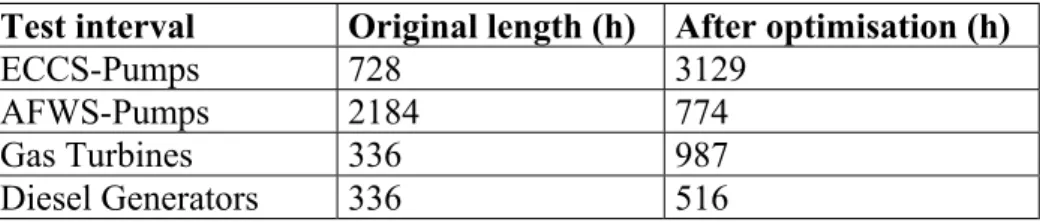
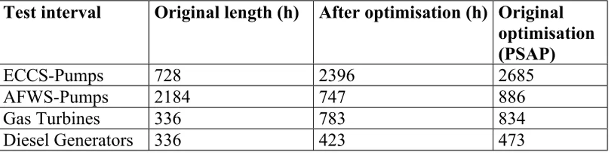
The result of the optimisation is presented in the tables below. In Table 1 the result of the optimisation using RiskSpectrum DOS is presented and in Table 2 the result of the optimisation using RiskSpectrum PSA Professional is presented.
Table 1: Original optimisation RiskSpectrum DOS
Test interval Original length (h) After optimisation (h)
ECCS-Pumps 728 3129 AFWS-Pumps 2184 774 Gas Turbines 336 987 Diesel Generators 336 516
Table 2: Original optimisation RiskSpectrum PSA Professional
Test interval Original length (h) After optimisation (h)
ECCS-Pumps 728 2685
AFWS-Pumps 2184 886 Gas Turbines 336 834 Diesel Generators 336 473
6.1.3 Discussion
The result of the optimisation is very interesting. If the test interval for the main pumps in the auxiliary feed water system (AFWS) is shortened from three months (2184 hours) to approximately one month the other three test intervals can be lengthened
significantly.
These rather dramatic changes in the test intervals will not affect the total frequency of loss of core cooling, it will remain constant, but the number of tests for these four systems will be almost half as many compared to before the optimisation.
6.1.3.1 Auxiliary Feed Water System (AFWS)
A possible reason for the large importance of the test interval for the AFWS is that both diesel generators and gas turbines back up the power supply. This means that the contribution of mechanical failures to the total unavailability of the system is high and the probability of mechanical failures is related to the length of the test interval
(Q=q+λt, see chapter 3.2).
Further, the AFWS in the Oskarshamn 1 power unit is separated from the other safety systems and therefore no dependencies between the AFWS and the other systems exist. This means that failure modes for components in the AFWS is present in a large number of cut-sets. For the other systems, failures in support systems or electrical power
systems may affect more than one safety system.
To illustrate why the test intervals for the AFWS are important the initiating event loss of offsite power can be studied. This initiating event contributes to approximately 20 percent of the total frequency of loss of core cooling. The cut-set list consists of a large number of events of the following kind:
− Loss of offsite power (initiating event)
− Common cause failure in diesel generators (DG111 and DG112) − Common cause failure in AFWS (two redundant trains)
Both diesel generators and gas turbines back up the AFWS. The other systems, for example the ECCS, are however not backed up by gas turbines and loss of offsite power in combination with failures in the diesel generators will therefor make these systems unavailable. This has the effect that component failures in the AFWS is present in a large number of cut-sets and since the test interval for the AFWS originally is three months this test interval is very important. The RDF is high which means that
immediately after periodic testing of the pumps in the AFWS the frequency of loss of core cooling is considerably lowered.
6.1.3.2 Diesel Generators and Gas Turbines
Failures in diesel generators and gas turbines are also present in a large number of cut-sets according to the discussion above. The test intervals for diesel generators and gas turbines are however two weeks so the RDF is not very large.
6.1.3.3 Emergency Core Cooling System (ECCS)
In the original analysis the RDF for the test interval for the ECCS-pumps is quite small, approximately 1.02-1.03, implying that these pumps are tested too often. There are several reasons for the small RDF.
The contribution from large LOCAs, where function of the ECCS is essential, is moderate in the PSA-analysis. The contribution to the total frequency is approximately 10%, which is relatively low compared to many other PSA-analyses. Another reason of the low RDF is found when examining the cut-set list for the system. The failures that contribute the most to the unavailability of the system are failures in components that are not tested when testing the pumps.
6.1.4 Differences Between RiskSpectrum DOS and PSAP
As seen in Table 1 and Table 2 the result differs when using different methods and software for calculating the importance of the test intervals.
There are several reasons for this. Firstly, when calculating all initiating events in one consequence analysis case the result will differ compared to when calculating the initiating events individually since a cut-off procedure has to be used in these complex calculations. When using probabilistic cut-off the structure of the analysed fault tree will affect the outcome of the analysis, especially if the PSA model is large. It should also be mentioned that the way of using cut-off is somewhat different in RiskSpectrum PSA Professional compared to RiskSpectrum DOS. For further details about the cut-off procedure see the theory manual for RiskSpectrum PSA Professional, [4].
Secondly, when analysing all initiating events in one consequence top event and then calculating importance measures the result will be different compared to calculating the importance “manually”. In the first case the importance is calculated by setting the test
same cut-set list. In the second case the importance is calculated by setting the
parameter for the test interval to zero and then perform a new minimal cut-set analysis. This is the most correct way of calculating the importance. However, the two different methods do not normally lead to any significant differences in the results.
Another difference, which may affect the result, is the treatment of CCF-events in RiskSpectrum DOS compared to RiskSpectrum PSAP. In RiskSpectrum DOS the parameters used for CCF are specified in the CCF-group and if a component is member of a CCF-group its individual parameters are read from the CCF-group and not from the basic event specification. In RiskSpectrum PSAP the parameters for the CCF are read from the first basic event that is included in the CCF-group.
Normally, this difference will not affect the calculations since in most cases all components included in a CCF-group have identical parameters (except time to first test, TF). The risk of making errors is reduced in RiskSpectrum PSAP since the analyst doesn’t have to specify any failure data parameters for the CCF.
6.2
Failure Data Uncertainties
6.2.1 Introduction
A basic assumption in surveillance test interval optimisation is that the component unavailability is dependent on the time between tests. The component unavailability is given by the formulas in chapter 3.2.
The Swedish T-book, [3], shows that some component unavailabilities are totally dependent on the length of the test interval, while other components have 60-70% contribution from the independent unavailability. This large difference in failure data indicates that the failure data is incomplete and that the division into time dependent and time independent can be questioned. In appendix 1 this phenomena is illustrated. For each parameter in the T-book the time dependent unavailability is calculated for a number of test intervals. The contribution from time dependent unavailability to the total unavailability is plotted against different lengths of test intervals.
The purpose of the appendix is to illustrate that the contribution from time dependent unavailability to the total unavailability varies greatly between different parameters. For some of the parameters presented in the T-book, e.g. for the gas turbines, only λ is available.
Many references only presents q or λ. In these cases, we have the same problem as above. In addition, ageing is not considered, i.e. increase of q and λ as the component becomes older.
The sensitivity of failure data is examined by changing the proportions between time dependent and time independent failure data, i.e. probability q and failure intensity λ, but keeping the total unavailability Qmean constant. A simple example shows how this is
Table 3: Example of how proportions between time dependent and time independent failure data is modified
Proportion λ (1/h) TI (h) q Qmean Percentage time
dependent unavailability Original (e.g. T-book) 1,0E-4 100 1,0E-2 ≈1,5E-2 33% 50% time dependent 1,5E-4 100 7,5E-3 ≈1,5E-2 50% 100% time dependent 3E-4 100 0 ≈1,5E-2 100% 6.2.2 Results
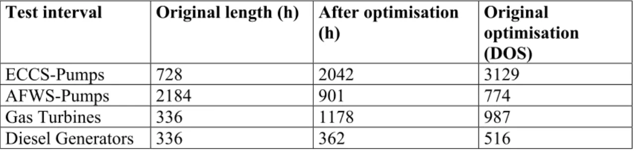
The result of the optimisation is shown in Table 4 and Table 5 below. In Table 4 the result of the optimisation when 50% of the total unavailability of the components are assumed to be time dependent is presented and the corresponding results with 100% time dependent failure data is presented in Table 5. The calculations have been performed using RiskSpectrum DOS.
Table 4: Failure data 50% time dependent
Test interval Original length (h) After optimisation (h) Original optimisation (DOS) ECCS-Pumps 728 2042 3129 AFWS-Pumps 2184 901 774 Gas Turbines 336 1178 987 Diesel Generators 336 362 516
Table 5: Failure data 100% time dependent
Test interval Original length (h) After optimisation (h) Original optimisation (DOS) ECCS-Pumps 728 2323 3129 AFWS-Pumps 2184 847 774 Gas Turbines 336 1241 987 Diesel Generators 336 451 516
The difference compared to the original optimisation is significant. In the original optimisation the test interval for ECCS is 3129 hours. The test interval for ECCS calculated with both 50% and 100% time dependent unavailability is significantly shorter.
6.2.3 Discussion
In the previous chapter the results of the optimisation with modified failure data was presented and relatively large differences between this optimisation and the original optimisation was noticed.
Although there is a difference in the results the main result is the same, i.e. as long as the test interval for the AFWS is shortened the other investigated test intervals can be prolonged.
It is not very surprising that the result of the optimisation will be different if the failure data is modified since the method is based on the formula Q(t)≈q+λt.
An aspect, which is not investigated in this analysis, is the effect of staggered testing since a mean MCS calculation technique is used. These analyses should therefor also be performed using time dependent calculations.
6.3
Deterministic Uncertainties
6.3.1 Introduction
Deterministic uncertainties must not be allowed to have too large influence on the optimisation results. One example of a deterministic uncertainty is whether the main feed water system is included in the PSA-analysis. The main feed water system is not classified as a safety system and is often not included in PSA models. The PSA model for the Oskarshamn 1 NPP is developed in order to obtain a complete and realistic reflection of the status of the power plant and therefor the main feed water system is taken into account.
In the PSA model used, the main feed water system is included and modelled in detail. It is of course not sufficient for all initiating events, e.g. large LOCAs. For most common cause initiators and transients it is included in the analysis since deterministic analyses show that the capacity and design of the system is sufficient.
Due to the level of detail of the PSA model a generic event tree can be used and whether the system is available or not is controlled by the logic in the fault trees.
For example, the initiating event loss of offsite power will make the main feed water system unavailable since there is no backup from diesel generators or gas turbines. In the event tree, however, the main feed water system is modelled as a function event since a generic event tree is used for all transients. When analysing the initiating event, a house event representing loss of offsite power is set to true making the main 6 kV bus bars unavailable and this in turn causes loss of power supply to the main feed water pumps.
There are a number of other initiating events that will make the main feed water system unavailable and this is, in the same manner as for loss of offsite power, controlled by the fault tree logic.
6.3.2 Result
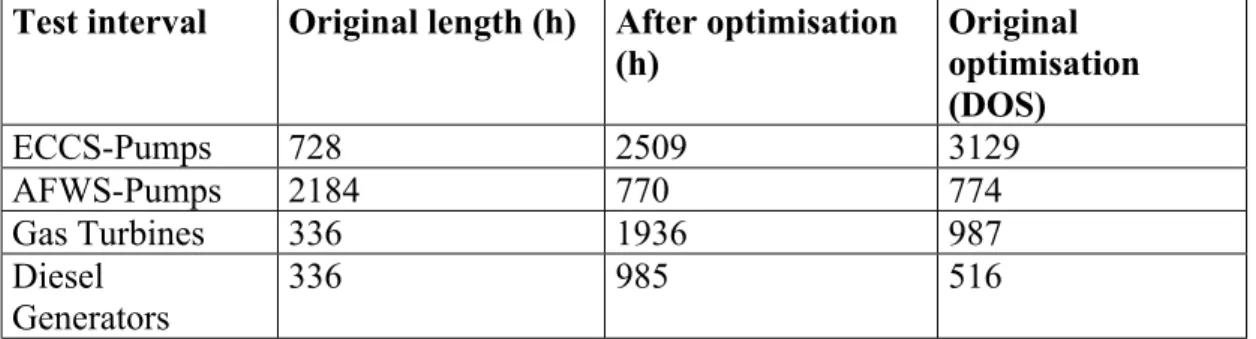
The result of the optimisation is shown in Table 6 below. The calculations have been performed using RiskSpectrum DOS.
Table 6: Result of optimisation when feed water system is not included in the PSA model
Test interval Original length (h) After optimisation (h) Original optimisation (DOS) ECCS-Pumps 728 2509 3129 AFWS-Pumps 2184 770 774 Gas Turbines 336 1936 987 Diesel Generators 336 985 516
As described in chapter 3 above, optimisation in this project means finding the optimal length of the test intervals at a given frequency of loss of core cooling. When the main feed water system is removed from the PSA model the frequency will of course raise. The optimisation is then performed using this new, higher frequency.
The analysis without the feed water system show large differences compared to the original optimisation. The test intervals for the gas turbines and diesel generators after optimisation are almost twice as long compared to the original optimisation.
6.3.3 Discussion
Although there is a difference in the results when the feed water system is not included the main result is the same, i.e. as long as the test interval for the AFWS is shortened the other investigated test intervals can be prolonged.
The large differences for the gas turbines and diesel generators show that the result of an optimisation largely depends on the assumptions regarding deterministic
uncertainties.
When examining the results in detail, some differences are noticed. Some initiating events that were important in the original analysis are now less important and vice versa. The dominating initiating event is still loss of offsite power. In the original analysis, after optimisation, the contribution to the total frequency of loss of core cooling from this initiating event was approximately 23%, now it is lowered to about 16%.
The cut-set lists are however quite similar. For the transients and common cause initiators on bus bars, a typical cut-set consists of events that make the power supply unavailable (offsite power and diesel generators) combined with common cause failure in the AFWS (alternatively failure in gas turbines).
6.4
Plant Configuration
6.4.1 Introduction
When performing a PSA-analysis normally only one plant configuration is analysed and many PSA models only allow one configuration to be analysed. It is however possible that the configuration affects the result.
The PSA model for Oskarshamn 1 NPP is adjusted to allow LPSA applications, meaning that a different configuration can be studied. For each modelled system with redundant components it is necessary to specify which components, e.g. pumps, that are running and which are in standby mode. It is also possible to make components, or trains, unavailable due to maintenance. When performing a risk follow up these adjustments have to be possible to make.
Two alternative plant configurations, aside from the one used in the original analysis, have been investigated. In Table 7 below the different plant configurations are shown.
Table 7: Investigated plant configurations
Configuration 1 (original) Configuration 2 Configuration 3
312P1, P2 312P2, P3 312P1, P3 442P1, P2 442P2, P3 442P1, P3 712P1, P2 712P2, P3 712P1, P3 712P4 712P5 712P5 715P1 715P2 715P2 721P1, P2 721P2, P3 721P1, P3 751F1 751F2 751F2 754F1 754F2 754F2 6.4.2 Results
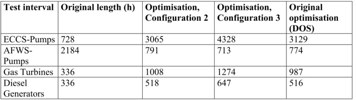
The results of the optimisations are shown in Table 8 below. The calculations have been performed using RiskSpectrum DOS.
Table 8: Results of optimisations when analysing different plant configurations
Test interval Original length (h) Optimisation, Configuration 2 Optimisation, Configuration 3 Original optimisation (DOS) ECCS-Pumps 728 3065 4328 3129 AFWS-Pumps 2184 791 713 774 Gas Turbines 336 1008 1274 987 Diesel Generators 336 518 647 516
The results of these optimisations are very interesting. The result when analysing configuration 2 is almost identical to the original optimisation. An optimisation with plant configuration 3 however, show large differences compared to the original optimisation.
Also the frequency of loss of core cooling differs between plant configuration 3 and the original configuration. It is somewhat higher when analysing configuration 3. Plant configuration 2 result in about the same frequency as the original configuration. It should be noted that the investigated plant configurations are only three configurations out of a large number of possible configurations.
6.4.3 Conclusions
Although there is a difference in the results for different configurations the main result is the same, i.e. as long as the test interval for the AFWS is shortened the other
investigated test intervals can be prolonged.
Since the optimisation of configuration 3 show large differences compared to the original optimisation these results must be investigated a bit further.
The contribution to the frequency of loss of core cooling from common cause initiators on bus bar is larger when analysing configuration 3 compared to the original
optimisation. This in turn has the effect that large LOCAs, where the ECCS is
important, contribute in a lesser amount to the total frequency. Therefor the test interval for the ECCS when analysing configuration 3 becomes even longer than in the original optimisation.
In this analysis two different configurations, aside from the original configuration, has been analysed. No in depth check of which configurations, except the original
configuration, that are actually used during normal operations has been done. Configuration 3 which showed the most difference compared to the original
optimisation is however not unrealistic. In the systems with three main pumps, e.g. the feed water system, part of the year pump P1 and pump P3 are used together.
There are a large number of possible configurations but when performing an actual optimisation it is of course only necessary to analyse the configurations that are used (which can be a large number). Since each optimisation is quite time consuming it is probably not possible to analyse all configurations. The number of sensitivity analyses of alternative configurations that has to be performed is dependent on the stability of the results.
6.5
Outage Times Caused By Test
6.5.1 Introduction
component may fail during the test which leads to that the component then becomes unavailable due to repair.
The unavailability due to maintenance for a periodically tested component is approximated by the following formula:
q0 = Time independent failure probability per demand
λSB = Stand by failure rate
MTTR = Mean time to repair TI = Test interval
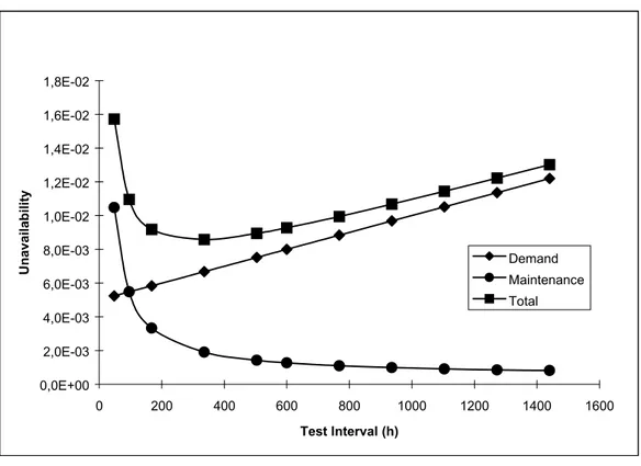
In Diagram 1 below the effect of different test intervals for a component is shown. The unavailability due to component failure (formula 1 in chapter 3.2), maintenance
(formula 5 above) and the sum are shown.
Diagram 1: Component unavailability
As seen in the diagram it is possible to calculate the optimal test interval for the single component. Such an approach leads to that optimal test intervals are determined for single components. An optimisation on a higher level (e.g. system or plant level) will probably result in different test intervals. That is, the optimal test interval for a single component is not necessarily optimal from the plant point of view.
TI MTTR TI q Qm =( s +λSB⋅ )⋅ 0,0E+00 2,0E-03 4,0E-03 6,0E-03 8,0E-03 1,0E-02 1,2E-02 1,4E-02 1,6E-02 1,8E-02 0 200 400 600 800 1000 1200 1400 1600 Test Interval (h) Unavailability Demand Maintenance Total (5)
The optimisations performed so far has not taken into account the fact that the component unavailability due to maintenance will change when adjusting the test intervals.
In this optimisation the unavailability due to maintenance will be adjusted. There are a number of factors that have to be taken into account when performing this analysis. It is possible in RiskSpectrum to assign a parameter for MTTR in the basic event for component failure. This presuppose that the component is only repaired when a critical failure occurs, which probably isn’t the case. In the original model the component unavailability due to maintenance is instead calculated manually and modelled in separate basic events. The calculated unavailability (using formula 5) is then multiplied with a factor 2 in order to take maintenance due to non-critical failures (e.g. a small leakage in a valve) into account.
The following adjustments have been performed. The unavailability due to maintenance has been adjusted by assigning MTTR to the basic event for component failure. This unavailability is dependent on the length of the test interval and thus represents unavailability due to critical failures. Further, a separate basic event is assigned an unavailability representing maintenance due to non-critical failures.
This way of modelling unavailability due to maintenance reduces the amount of work. The unavailability due to maintenance caused by critical failures will automatically be updated when the test interval is changed. At the same time the unavailability due to maintenance caused by non-critical failures will remain constant (modelled in a separate basic event).
6.5.2 Results
The result of the optimisation is shown in Table 9. The calculations have been performed using RiskSpectrum PSAP.
Table 9: Result of optimisation with adjusted maintenance unavailability
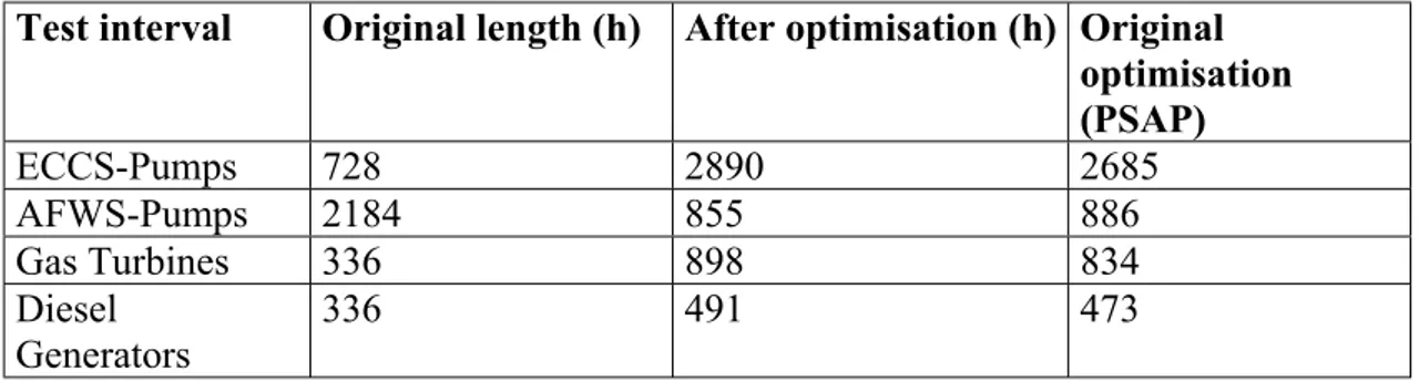
Test interval Original length (h) After optimisation (h) Original optimisation (PSAP) ECCS-Pumps 728 2890 2685 AFWS-Pumps 2184 855 886 Gas Turbines 336 898 834 Diesel Generators 336 491 473
The result of the optimisation shows that the test intervals generally are somewhat longer when adjusting the maintenance unavailability.
The total frequency of loss of core cooling becomes slightly higher in this optimisation. A probable explanation is that the basic event representing component failure now also
Due to the complex fault tree model a cut off has to be used to reduce the computational work. The component failure basic events have a higher unavailability when including MTTR and the cut sets including these basic events are thus less likely to be thrown away due to cut off.
6.5.3 Conclusions
The tendency of obtaining longer test intervals when adjusting the unavailability due to maintenance is expected. The objective with the optimisation is to minimise the number of tests and at the same time keep the total risk constant. The test intervals are thus lengthened after an optimisation and a longer test interval will reduce the unavailability due to maintenance. In order to keep the risk at a constant level the test intervals can be additionally lengthened compared to the original optimisation.
The difference in results are however small. The test interval for the ECCS becomes approximately 8% longer and the other test intervals are almost the same compared to the original optimisation.
6.6
Calculation Technique
6.6.1 Introduction
One area, which is very important to study when performing an optimisation of test intervals, is calculation technique. The analyses performed in the previous chapters are mean MCS-calculations. The advantage with the MCS analysis is the calculation of sensitivity measures (e.g. RDF). The disadvantage is that staggered testing is incorrectly treated. By performing a time dependent analysis the effect of staggered testing will be handled in a correct manner. In the time dependent analysis it is assumed that when a test is made on one component in a CCF-group, the probability for all CCF-events involving the component becomes equal to a base line time independent CCF probability.
The time dependent calculation uses the cut set list produced in a MCS analysis. For each time point the top event is calculated and the variation of the top event frequency can therefor be studied over a period of time.
To determine the importance of a test interval in a time dependent analysis the following steps are gone through:
− Calculate the original mean unavailability using time dependent analysis. All initiating events have to be calculated in one top event for the result to be relevant. − Set the test interval, for which the importance is to be calculated, to zero and
recalculate the mean unavailability using time dependent analysis.
− The importance (RDF) of the test interval is obtained by dividing the original result with the result with the test interval set to zero.
This procedure of calculating importance of test intervals is much more time consuming since a separate analysis has to be performed for each test interval.
In this study four test intervals are analysed. To calculate the importance of these test intervals using MCS mean analysis only one MCS calculation has to be performed. The importance of the test intervals are then obtained by manipulating the cut set list. When calculating the importance using time dependent analysis five separate MCS analyses, one original analysis and one for each test interval set to zero, have to be performed. The LPSA model used is quite large and the computational work is hence substantial. The process of optimisation requires several iterations. If, for instance, five iterations are necessary to obtain optimal test intervals, 25 MCS calculations have to be performed when using a time dependent approach. If a MCS mean analysis is used instead only five MCS calculations are necessary.
Of the test intervals studied in this optimisation, the tests for the AFWS pumps and diesel generators are staggered. The tests for the ECCS and gas turbines are sequential. A simple example shows the effect of staggered versus sequential testing when using different calculation techniques.
6.6.1.1 Example Time Dependent Calculations
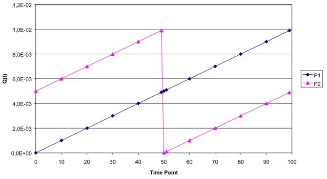
The unavailability of two pumps, P1 and P2, are calculated and the top event is “Both P1 and P2 fail”. The parameters used in the calculations are shown in Table 10 below.
Table 10: Parameters in example for calculation technique
Pump P1 Pump P2
Failure Intensity, λ (1/h) 1E-4 1E-4 Test Interval, TI (h) 100 100 Time to First Test, TM (h) 50 0
Diagram 2: Example of time dependent unavailabilities for P1 and P2
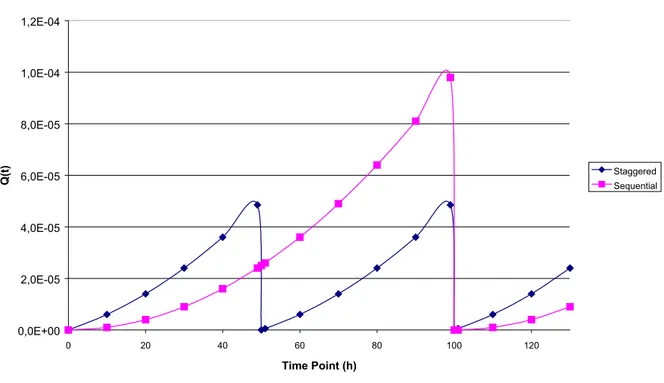
In Diagram 3 the total unavailability for the top event “Both P1 and P2 fail” is shown. The effect of staggered testing versus sequential testing is obvious.
Unavailability P1 and P2 0,0E+00 2,0E-03 4,0E-03 6,0E-03 8,0E-03 1,0E-02 1,2E-02 0 10 20 30 40 50 60 70 80 90 100 Time Point Q(t) P1P2
Diagram 3: Example staggered testing versus sequential testing
When performing an MCS mean analysis the mean unavailability for each component is calculated according to formula 3 in chapter 3.2. For the pumps in this example the following mean value is obtained using this formula:
Qmean=4,98E-3
The mean unavailability for the top event “Both P1 and P2 fail” is approximately: Qmean, TOP=4,98E-3*4,98E-3=2,48E-5
This is the result obtained when performing a mean MCS-calculation. The effect of the staggered testing is not taken into account.
When performing a time dependent analysis the unavailability at the time point T for the top event is calculated according to2:
QMCS, i is calculated using formula 1 in chapter 3.2.
∏
= − − = n i i MCS TOP T Q T Q 1 , ( )) 1 ( 1 ) ( (6) Unavailability P1 and P2 0,0E+00 2,0E-05 4,0E-05 6,0E-05 8,0E-05 1,0E-04 1,2E-04 0 20 40 60 80 100 120 Time Point (h) Q(t) StaggeredSequentialThe mean unavailability is calculated by integration and time averaging of QTOP(T):
The mean unavailability that is calculated in a time dependent analysis is therefor different compared to the unavailability calculated in the MCS-analysis.
For the example with the pumps P1 and P2 above, the following result will be achieved3:
QTOP, mean=1,73E-5 (staggered testing)
This result is lower than the mean unavailability calculated in the MCS mean analysis. If the pumps are tested sequentially, i.e. no staggering, the result will be:
QTOP, mean=3,41E-5 (sequential testing)
This result on the other hand is somewhat higher than the mean unavailability calculated in the MCS mean analysis.
The results of the calculations in this example are put together in Table 11.
Table 11: Results of calculations in example
MCS mean analysis Time Dependent Analysis
Test Procedure - Staggered Sequential Qmean 2,48E-5 1,73E-5 3,41E-5
As seen the results differ depending on calculation technique and test procedure. All the analyses so far have been mean MCS analyses. In this chapter, an optimisation have been performed using time dependent calculations.
6.6.2 Result
The result of the optimisation is shown in Table 12 below. The calculations have been performed using RiskSpectrum PSAP.
3 The integration is carried out numerically by using linear approximation between the time points and the
result of the integration is thus not exact.
∫
= T TOP mean TOP Q t dt T Q 0 , ( ) 1 (7)Table 12: Result of optimisation using time dependent calculations
Test interval Original length (h) After optimisation (h) Original optimisation (PSAP) ECCS-Pumps 728 2396 2685 AFWS-Pumps 2184 747 886 Gas Turbines 336 783 834 Diesel Generators 336 423 473
The result of the optimisation using time dependent calculation show that the test intervals are generally shorter, i.e. the optimisation is not as effective compared to the original optimisation. Although the test interval for the AFWS is additionally shortened in the time dependent analysis, the other test intervals are also shorter. This implies that the tests are not as important when using time dependent calculations.
6.6.3 Conclusions
The effect of a test in terms of risk reducing capacity is lower in this analysis when time dependent calculation technique is used. This might depend on the fact that the tests for the AFWS and diesel generators are staggered. In the time dependent analysis the staggering is taken into account. The risk profile becomes “smoother” when the tests are staggered, see Diagram 3 in chapter 6.6.1.1.
This may result in less dramatic changes in the lengths of test intervals when a time dependent analysis is performed.
The differences are quite small and a time dependent calculation might therefor be used as a confirmatory analysis. That is, first a number of sensitivity analyses are performed, e.g. failure data uncertainties and deterministic uncertainties, in order to form an idea of the magnitude of the optimal test intervals. After that, a time dependent calculation might be performed to insure that the results do not change dramatically.
7
Summary of Results
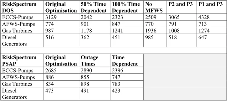
The results of the optimisations are summarised in the Table 13 below.
Table 13: Summary of optimisation results
RiskSpectrum DOS Original Optimisation 50% Time Dependent 100% Time Dependent No MFWS P2 and P3 P1 and P3 ECCS-Pumps 3129 2042 2323 2509 3065 4328 AFWS-Pumps 774 901 847 770 791 713 Gas Turbines 987 1178 1241 1936 1008 1274 Diesel Generators 516 362 451 985 518 647 RiskSpectrum PSAP Original Optimisation Outage Times Time Dependent ECCS-Pumps 2685 2890 2396 AFWS-Pumps 886 855 747 Gas Turbines 834 898 783 Diesel Generators 473 491 423
These results are also shown in Diagram 4 and Diagram 5 below where the differences between the analyses are visualised.
Optimisation DOS P1, P3 P2, P3 No MFWS 100% Time 50% Time Original (DOS) 0 500 1000 1500 2000 2500 3000 3500 4000 4500 5000 Analysis Test Interval ECCS AFWS Gas Turbines Diesel Generators
Diagram 4: Results of optimisation (RiskSpectrum DOS)
Optimisation PSAP Time Dep. Maintenance Original (PSAP) 0 500 1000 1500 2000 2500 3000 3500 Analysis Test Interval ECCS AFWS Gas Turbines Diesel Generators
Diagram 5: Results of optimisation (RiskSpectrum PSAP)
It is clear that different modelling technique and assumptions affect the result of an optimisation. The main result is however the same for all optimisations, namely that the test intervals for the ECCS, gas turbines and diesel generators can be lengthened if only the test interval for the AFWS is shortened. The effect of the optimisation will then be a
However, some differences should be noticed:
− The result is sensitive to failure data, i.e. the failure data must be gathered from reliable sources.
− If the main feed water system is excluded, the test intervals for the gas turbines and diesel generators will be significantly longer, i.e. it is important that the LPSA model is not overly conservative.
− Plant configuration may affect the outcome of an optimisation and several alternatives should be investigated.
7.1
Discussion of Results
The optimisation of the investigated test intervals results in rather dramatic changes, which indicates that the test intervals before the analysis definitely was non-optimal. The test interval for the ECCS was too short and the test interval for the AFWS was too long.
The ECCS is important after large LOCAs but the PSA analysis shows that the contribution from large LOCAs to the total frequency of loss of core cooling is moderate. The AFWS, on the other hand, is separated from the remaining safety systems and no dependencies between the AFWS and the other systems exist. The capacity of the AFWS is sufficient for most of the important initiating events, e.g. transients and CCIs.
The sensitivity analyses show that the exact lengths of the optimised test intervals are difficult to determine. However, the optimisation indicates in what range an optimised test interval should be. If using risk based optimisation a set of sensitivity analyses has to be performed.
If the results of an optimisation, including sensitivity analyses, are treated correctly, more optimal test intervals can be determined. In the next chapter some alternatives are evaluated.
7.1.1 Investigation of Alternative Test Intervals
In this chapter the procedure of how to choose which test intervals to use when performing a risk based optimisation of the technical specifications is treated. The purpose is not to suggest actual changes but instead to discuss how to treat results from an optimisation.
Table 14: Range of test intervals after optimisation
Test Interval Original Length (h) After Optimisation (h)
ECCS-Pumps 728 2042-4328 AFWS-Pumps 2184 713-901 Gas Turbines 336 783-1936 Diesel Generators 336 362-985
The main question after performing an original optimisation and a number of sensitivity analyses will of course be which results to use.
An important aspect is the administrative and practical considerations that have to be made. The test schemes must for instance be on a weekly basis.
The test interval for the ECCS after optimisation is ranging from approximately 2000 hours to 4000 hours. The shortest test intervals are obtained when changing the failure data and the longest test interval when analysing an alternative configuration. A possible choice would be approximately 2500 hours since the optimisation using time dependent calculations yielded a result of approximately 2400 hours. In this calculation the effect of changed unavailability due to testing was not included and a time
dependent optimisation, with the dynamic test unavailability included, would lead to slightly longer test intervals.
The test interval for the AFWS is less sensitive for changes in the assumptions so the range of calculated test intervals is quite small. Two possible choices appear, four weeks (672 hours) and five weeks (840 hours). Which one to choose is a matter of administrative considerations.
The test interval for the gas turbines became significantly longer when optimising without including the main feed water system (deterministic uncertainties). For the other optimisations the range was from approximately 800 hours to 1300 hours. The longest test intervals were obtained when the failure data was manipulated and when an alternative configuration was analysed. A test interval in the range of five to eight weeks (840 to 1344 hours) is a possible choice. An additional consideration that has to be made regarding the gas turbines is that these are actually shared with the Oskarshamn 2 NPP and an optimisation of the test intervals of Oskarshamn 2 would perhaps lead to a different result.
Finally, the optimisation of the test interval for the diesel generators lead to results in the range of 362-985 hours. The longest test interval is obtained when excluding the main feed water system in the analysis. Here, possible choices are two to fours weeks (336 to 672 weeks). The original length, before optimisation, is two weeks and perhaps a change would not be necessary for the diesel generators.
Table 15: Evaluation of two alternative test schemes
Test Interval Before
Optimisation (h) Alternative 1 (h) Alternative 2 (h)
ECCS-pumps 728 3000 2500
AFWS-pumps 2184 840 672
Gas Turbines 336 1344 840 Diesel Generators 336 672 336
Nominal Values
Loss of Core Cooling 1,0 1,07 0,92 Number of Tests 1,0 0,48 0,78
Alternative 1 is a non-conservative choice where the test intervals have been chosen as long as possible. The total frequency of loss of core cooling thus becomes somewhat higher compared to the original frequency but on the other hand the number of tests are significantly decreased.
Alternative 2 is a conservative choice where the test intervals are relatively short. This alternative also gives a decreased number of tests, and the frequency of loss of core cooling is actually lower than before the optimisation.
8
Conclusions
This work shows that the results of an optimisation of surveillance test intervals are affected by the assumptions made in the model and also by failure data uncertainties. The differences in results are in some cases significant but the fundamental results remains.
In order to determine optimal surveillance test intervals a number of sensitivity analyses should be performed. Together with the original optimisation, a set of sensitivity
analyses form a picture of the stability of the results.
In this work the following sensitivity analyses had a relatively large impact on the results:
− Failure data uncertainties − Deterministic uncertainties − Plant configuration
When performing an optimisation it is therefor recommended to investigate these areas. The calculation technique, MCS mean analysis versus time dependent analysis, did not significantly affect the optimisation result and it is not considered necessary to perform time dependent analyses, based on the results in this report.
An area which probably needs to be investigated a bit further is the importance of completeness of the LPSA model. The model used so far is quite large with a very
detailed modelling of support and electrical systems. It would for instance be of interest to investigate how the optimisation results are affected if some simplifications are made: − Replace some electrical or support systems with single basic events
− Simplify the modelling of actuating and isolation signals
− Analyse the frequency of loss of core cooling without common cause initiators (CCI) as initiating events
9
References
[1] Johanson, G., and Holmberg, J., Safety Evaluation by Living Probabilistic
Safety Assessment, SKI Report 94:2, Swedish Nuclear Power Institute,
Stockholm 1994.
[2] Sandstedt, J., Pilot Study: Analysis of Prescribed Test Intervals, Oskarshamn 2, SKI Report 94:4, Swedish Nuclear Power Institute, Stockholm 1994.
[3] T-book, 4th edition, Reliability Data of Components in Nordic Nuclear Power Plants, ATV-kansliet and Studsvik AB, ISBN 91-7186-303-6
Appendix 1 Pe rc entage Time Depende nt U n a va ila bility