Report number: 2011:29 ISSN: 2000-0456
Research and Development Program
in Reactor Diagnostics and Monitoring
with Neutron Noise Methods, Stage 17
2011:29
Author: Imre Pázsit
Tran Hoai Nam Victor Dykin Anders Jonsson
SSM perspective
Background
This report constitutes Stage 17 of a long-term research and develop-ment program concerning the developdevelop-ment of diagnostics and monito-ring methods for nuclear reactors.
Results up to Stage 16 were reported in SKI and SSM reports, as listed below and in the Summary. The results have also been published in international journals and have been included in both licentiate- and doctor’s degrees.
Objectives of the project
The objective of the research program is to contribute to the strate-gic research goal of competence and research capacity by building up competence within the Department of Nuclear Engineering at Chalmers University of Technology regarding reactor physics, reactor dynamics and noise diagnostics. The purpose is also to contribute to the research goal of giving a basis for SSM’s supervision by developing methods for identification and localization of perturbations in reactor cores.
Results
The program executed in Stage 17 consists of the following three parts: • Development of the noise simulator, CoreSim, to effectively model
the noise induced by vibrating fuel assemblies, for the calculation of ex-core detector noise;
• Extension of the traditional Rossi-alpha method to two energy groups;
• Study of the dynamics of liquid fuel systems: extension of the mo-del to two energy groups.
Project information
Responsible at SSM has been Ninos Garis.
SSM references: SSM 2009/2093, SSM 2010/2134
Previous SKI reports: 95:14 (1995), 96:50 (1996), 97:31 (1997), 98:25 (1998), 99:33 (1999), 00:28 (2000), 01:27 (2001), 2003:08 (2003), 2003:30 (2003), 2004:57 (2004), 2006:34 (2006), 2008:39 (2008), Previous SSM reports: 2009:38 (2009), 2010:22 (2010)
2011:29
Authors: Imre Pázsit, Tran Hoai Nam, Victor Dykin and Anders JonssonChalmers University of Technology, Department of Nuclear Engineering, Göteborg
Date: May 2011
Report number: 2011:29 ISSN: 2000-0456
Research and Development Program
in Reactor Diagnostics and Monitoring
with Neutron Noise Methods, Stage 17
This report concerns a study which has been conducted for the Swedish Radiation Safety Authority, SSM. The conclusions and view-points presented in the report are those of the author/authors and do not necessarily coincide with those of the SSM.
Contents
Contents ... 1
Summary ... 3
Sammanfattning ... 6
1 Development of the noise simulator, CoreSim, to effectively model the noise induced by vibrating fuel assemblies, for the calculation of ex-core detector noise ... 9
1.1 Introduction ... 9
1.2 Calculation of the neutron noise at an ex-core position ... 10
1.3 Results of the calculated case in 1-D ... 12
1.4 Conclusions ... 18
2 Extension of the traditional Rossi-alpha method to two energy groups ... 19
2.1 Abstract ... 19
2.2 A simple stochastic model ... 21
2.2.1 Backward Kolmogorov equations ... 22
2.2.2 Calculation of the expectation of the number of fast neutrons. ... 23
2.3 Time correlation neutron counting with triggering on the spontaneous fission events - the Rossi-alpha formula in two groups ... 25
2.4 Discussion and conclusions ... 30
3 Study of the dynamics of liquid fuel systems: extension of the model to two energy groups ... 31
3.1 Introduction ... 31
3.2 Two-group equations ... 31
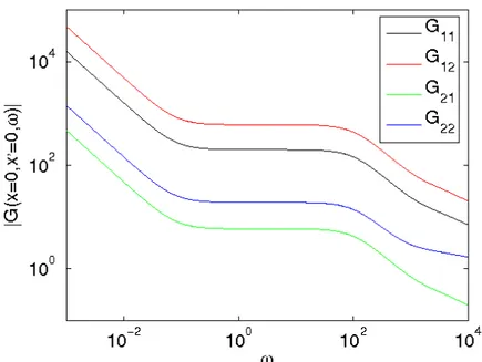
3.3 The Green’s function ... 32
3.4 Propagating perturbation ... 35
3.5 Space dependence of the noise induced by propagating perturbations ... 38
3.6 Finite velocity ... 40
3.7 Conclusions ... 43
Acknowledgement ... 45
References ... 45
Summary
This report gives an account of the work performed by the Department of Nuclear Engineering, Chalmers University of Technology, in the frame of a research contract with the Swedish Radiation Safety Authority (SSM), contract No. SSM 2010/2134. The present report is based on work performed by Imre Pázsit, Tran Hoai Nam, Victor Dykin and Anders Jonsson, with Imre Pázsit being the project leader.
This report describes the results obtained during Stage 17 of a long-term research and development program concerning the development of diagnostics and monitoring methods for nuclear reactors. The long-term goals are elaborated in more detail in e.g. the Final Reports of Stages 1 and 2 (SKI Report 95:14 and 96:50, Pázsit et al. 1995, 1996). Results up to Stage 16 were reported in (Pázsit et al. 1995, 1996, 1997, 1998, 1999, 2000, 2001, 2003a, 2003b; Demazière et al, 2004; Sunde et al, 2006: Pázsit et al. 2008, 2009, 2010).
The program executed in Stage 17 consists of three parts as follows:
• Development of the noise simulator, CoreSim, to effectively model the noise induced by vibrating fuel assemblies, for the calculation of ex-core detector noise; • Extension of the traditional Rossi-alpha method to two energy groups;
• Study of the dynamics of liquid fuel systems: extension of the model to two energy groups.
The work performed in each part is summarized below.
1. Development of the noise simulator, CoreSim, to effectively model the noise induced by vibrating fuel assemblies, for the calculation of ex-core detector noise
In the research project run in collaboration with Ringhals, we found that the amplitude of the peak in the ex-core neutron APSDs, corresponding to the beam mode vibrations of the core barrel, increases during the cycle, but returns to the initial value after refuelling, at the beginning of the next cycle. The reason for this behaviour is not understood. One guess, expressed by experts in the field, is that the scaling factor between core barrel displacement and the normalised neutron noise changes with the change of the boron content and flux redistribution in the core due to burn-up. We have investigated whether such a statement could be confirmed by the use of the noise simulator, developed at the Department (Demazière 2004, 2011). However, we did not find any increase of the normalised noise with constant vibration amplitude during the cycle when the noise induced by the vibrations of the core barrel was calculated (Pázsit et al., 2008).
In some recent work (Pázsit et al., 2008, 2010) we have arrived at the conclusion that the 8 Hz peak in the ex-core spectra, corresponding to the beam mode, consists of two peaks close to each other in frequency. The two peaks have different origins and different time evolution during the cycle. The peak closer to 7 Hz is induced by the core barrel vibrations, and its amplitude does not change significantly during the cycle. The
peak close to 8 Hz is due to the individual fuel assembly vibrations, and its amplitude increases monotonically during the cycle.
The fact that vibrations of individual fuel assemblies can contribute to the ex-core noise has been suggested already by Sweeney et al (1985). These authors also claim that the ex-core noise induced by such vibrations increases during the cycle due to the change of boron concentration and burn-up effects.
The purpose of the work in this Section is to investigate the possibility to confirm the validity of this statement with the use of the noise simulator. To this end the treatment of the vibrating control or fuel rod has to be improved compared to the default application. Instead of solving the noise equations with the actual noise source included, CORE SIM will be used to calculate the Green’s function, and the noise will be derived by a numerical integration of the Green’s function with the noise source representation. This way vibrations with a smaller amplitude can be treated than in the previous cases. In this Stage this methodology will be tested in a one-dimensional model for one single core configuration. The extension to 2-D and to the case of increasing burn-up will be performed in later work.
2. Extension of the traditional Rossi-alpha method to two energy groups
The traditional methods using higher moments of the detector counts, notably the Feynman- (variance to mean) and Rossi-alpha (temporal correlations) methods, are based on an energy-independent, or one-group, theory. The corresponding Feynman- and Rossi-alpha formulae were thus derived in a one-group theory setting. This energy-independent approach was experimentally justified since the methods appear to work well in a wide range of cases in thermal, water moderated systems, with a long thermal neutron lifetime and the dominance of the thermal flux.
However, there have been an increasing number of indications that in certain situations the traditional description may not work satisfactorily, in particular in fast systems and in reflected cores. From the experimental point of view, in several measurements it was found that the temporal behaviour of the Feynman- or Rossi-alpha measurements could not be fitted by one single exponential, rather two, or sometimes even more, exponential terms and corresponding exponentials were needed.
The simplest way of accounting for spectral effects and describing multi-alpha modes is to extend the theory of the Feynman- and Rossi-alpha methods to two energy groups, still in the same space-independent model as in the traditional works. With this extension, if one disregards the delayed neutrons, the temporal behaviour will be determined by two exponentials, and the whole theory still remains manageable fully analytically.
In this Stage therefore we will elaborate the theory of neutron fluctuations, more concretely that of the Rossi-alpha formula, in a two group approach with the master equation technique. Preliminary results were already obtained (Pál and Pázsit, 2011). Here we give the basics of the theory of the two-group version of the Rossi-alpha formula, with the first results. The calculations for the Rossi-alpha formula show that the temporal dependence of the detection rate of fast neutrons at time t+τ, following a triggering detection at time t indeed has a form of the sum of two exponentials. The
explicit form of the two-group Rossi-alpha formula is given and some possible further applications of the method are discussed.
3. Study of the dynamics of liquid fuel systems: extension of the model to two energy groups
In the previous reports, Stages 14-15 and 16, a simple one-dimensional one energy group model with propagating fuel properties was set up and studied as a model of a molten salt reactor. The solution of the static eigenvalue equation was given first by expansions into eigenfunctions of a corresponding traditional reactor, i.e. an reactor with fuel velocityu = . The noise was then calculated in Stage 16 by using a semi-0 analytical technique, where part of the flux was given as an exact solution of part of the problem, and the remainder was given as a series expansion. Doing so, several new features compared to the simpler approach presented in Stage 14 appeared, most notably a series of peaks in the frequency dependence. Further, the general behaviour of the reactor was found to be more point-kinetic than a corresponding traditional reactor. Finally, the noise from a propagating perturbation was calculated and was found to display some interesting features. The new findings were summarized in a recent journal publication (Pázsit and Jonsson, 2011).
To further improve on these results, for Stage 17, two-group theory was used. The techniques used for the one-group theory proved still to be useful to obtain solutions for the Green’s functions and the neutron noise. The new effects that are possible to study in a two-group approach are the presence and the significance of the local component, and the spectral effects (energy dependence) of the static flux and the neutron noise. In particular, in a two-group treatment it is possible to study the significance of the different fuel types and spectra on the induced neutron noise and its kinetic properties. Hence in this Stage, calculations were performed on three different systems: a thorium-fuelled thermal MSR, a thermal uranium reactor (based on data from Ringhals 1), and a fast high-conversion reactor. The results from these three systems were quantitatively compared. A more detailed description of the results are given in a new publication (Jonsson and Pázsit, 2011).
Sammanfattning
Denna rapport redovisar det arbete som utförts inom ramen för ett forskningskontrakt mellan Avdelningen för Nukleär Teknik, Chalmers tekniska högskola, och Strålsäkerhetsmyndigheten (SSM), kontrakt Nr. SSM 2010/2134. Rapporten är baserad på arbetsinsatser av Imre Pázsit, Tran Hoai Nam, Victor Dykin och Anders Jonsson, med Imre Pázsit som projektledare.
Rapporten beskriver de resultat som erhållits i etapp 17 av ett långsiktigt forsknings- och utvecklingsprogram angående utveckling av diagnostik och övervakningsmetoder för kärnkraftsreaktorer. De långsiktiga målen har utarbetats noggrannare i slutrapporterna för etapp 1 och 2 (SKI Rapport 95:14 och 96:50, Pázsit et al. 1995, 1996). Uppnådda resultat till och med etapp 16 har redovisats i referenserna (Pázsit et al, 1995, 1996, 1997, 1998, 1999, 2000, 2001, 2003a, 2003a; Demazière et al, 2004; Sunde et al, 2006; och Pázsit et al, 2008, 2009, 2010).
Det utförda forskningsarbetet i etapp 17 består av de tre följande delarna:
• Vidareutveckling av brussimulatorn CoreSim, för att effektivt kunna modellera bruset från vibrerande styrstavar och bränslepatroner i beräkningar av detektorbrus utanför härden;
• Utvidgning till två energigrupper av den vanliga Rossi-alpha-metoden;
• Studie av dynamiken hos system med flytande bränsle: utvidgning till två energigrupper av modellen.
Det utförda arbetet i varje del summeras nedan.
1. Vidareutveckling av brussimulatorn CoreSim, för att effektivt kunna modellera bruset från vibrerande styrstavar och bränslepatroner i beräkningar av detektorbrus utanför härden
I vårt forskningssamarbete med Ringhals fann vi att amplitudtoppen hos APSD-neutrondetektorerna utanför härden, som svarar mot reaktortankens ”beam mode”-vibrationer, ökar under cykeln, men återgår till ursprungsvärdet i början av nästa cykel efter bränslebyte. Orsaken till detta beteende är inte känd. En gissning, som framförts av experter inom området, är att skalfaktorn mellan reaktortankens förflyttning och det normaliserade neutronbruset ändras med förändring av borinnehållet och flödesförändring i härden på grund av utbränning. Vi har undersökt huruvida ett sådant påstående kan bekräftas genom att använda den brussimulator som utvecklats på institutionen (Demazière 2004, 2011). När vi beräknade bruset, som inducerats av reaktortankens vibrationer, kunde vi emellertid inte finna någon ökning av det normaliserade brus, som har konstant vibrationsamplitud, under cykeln (Pázsit et al., 2008).
I några nyare arbeten (Pázsit et al., 2008, 2010) har vi kommit till slutsatsen att toppen på 8 Hz i spektret utanför härden, som svarar mot ”beam mode”, består av två toppar , som ligger nära varandra i frekvens. De två topparna har olika ursprung och olika tidsutveckling under cykeln. Toppen närmare 7 Hz induceras av reaktortankvibrationer
och dess amplitud ändras inte signifikant under cykeln. Toppen nära 8 Hz beror på vibrationer i individuella bränsleknippen och dess amplitud ökar monotont under cykeln. Det faktum att vibrationer i individuella bränsleknippen kan bidra till brus utanför härden föreslogs redan av Sweeney et al (1985). Dessa författare hävdar också att det av sådana vibrationer inducerade bruset utanför härden ökar under cykeln på grund av ändringen i borkoncentration och utbränningseffekter.
Målsättningen med detta avsnitt är att undersöka möjligheten att bekräfta giltigheten hos detta påstående med hjälp av brussimulatorn. För detta ändamål måste behandlingen av vibrerande kontroll- eller bränslestavar förbättras jämfört med standardapplikationen. Istället för att lösa brusekvationerna med det aktuella bruset inkluderat, så ska CORE SIM användas för att lösa Greens funktion. Bruset erhålls sedan genom en numerisk integration av Greens funktion med bruskällerepresentation. På detta sätt kan vibrationer med mindre amplitud behandlas än i tidigare fall. I denna etapp ska denna metod testas på en endimensionell modell av en enstaka härdkonfiguration. Utveckling till två dimensioner och till fallet med ökande utbränning ska utföras i senare arbeten.
2. Utvidgning till två energigrupper av den vanliga Rossi-alpha-metoden
De traditionella metoderna använder högre moment av detektorsignalerna, i synnerhet Feynman- (varians till medelvärde) och Rossi-alphametoderna (tidskorrelationer), och är baserade på en energioberoende teori eller engruppsteori. Motsvarande Feynman- och Rossi-alphaformler härleddes alltså för engruppsteori. Denna energioberoende taktik motiverades experimentellt eftersom metoderna verkar fungera bra i ett stort antal fall för termiska, vattenmodererade system där man har lång termisk neutronlivslängd och dominans av termiskt flöde.
Det har emellertid framkommit ett ökande antal indikationer att i vissa situationer fungerar inte den traditionella beskrivningen tillfredsställande, speciellt inte i snabba system eller för härdar med reflektor. Från experiment fann man att vid åtskilliga mätningar kunde tidsbeteendet hos Feynman- eller Rossi-alphamätningarna inte anpassas till en enda exponentialfunktion, snarare behövdes två och ibland fler exponentialtermer och motsvarande exponentialfunktioner.
Det enklaste sättet att ta hand om spektraleffekter och att beskriva flera alphamoder är att utveckla teorierna för Feynman- och Rossi-alphametoderna till två energigrupper men fortfarande använda samma rumsoberoende modell som i de traditionella arbetena. Med denna utvidgning bestäms temperaturbeteendet av två exponentialfunktioner och hela teorin blir fortfarande fullt analytiskt hanterbar, om man bortser från de fördröjda neutronerna.
I denna etapp utarbetar vi därför i detalj teorin för neutronfluktuationer, mer konkret Rossi-alphaformeln, genom masterekvationsteknik för två grupper. Preliminära resultat hade redan tidigare uppnåtts (Pál and Pázsit, 2011). Här ger vi grunderna för tvågruppsteorin för Rossi-alphaformeln med de första resultaten. Beräkningarna med Rossi-alphaformeln visar att temperaturberoendet hos detekteringshastigheten för snabba neutroner vid tiden t+τ , som följer en triggningssignal vid tiden t verkligen har formen av summan av två exponentialfunktioner. Den explicita formen av
alphaformlen för två grupper ges och några möjliga ytterligare applikationer av metoden diskuteras.
3. Studie av dynamiken hos system med flytande bränsle: utvidgning till två energigrupper av modellen
I de tidigare rapporterna, etapp 14-15 och 16, ställdes en enkel endimensionell modell för en energigrupp och rörligt bränsle upp och studerades som modell för en saltsmältereaktor. Lösningen till den statiska egenvärdesekvationen gavs först i utvecklingar av egenfunktioner till en motsvarande traditionell reaktor, dvs. en reaktor med bränslehastighet u = . Bruset beräknades sedan i etapp 16 genom att använda en 0 halvanalytisk teknik, där en del av flödet gavs som en exakt lösning till en del av problemet, och resten gavs som en serieutveckling. Genom detta förfarande upptäcktes flera nya egenheter jämfört med det enklare förfarandet från etapp 14, varav det märkligaste var en serie toppar hos frekvensberoendet. Vidare befanns reaktorns allmänna beteende vara mer punktkinetiskt än en motsvarande traditionell reaktor. Slutligen beräknades bruset från en rörlig störning och detta befanns ha några intressanta karaktäristika. De nya resultaten summerades nyligen i en tidskriftspublikation (Pázsit and Jonsson, 2011).
För att ytterligare förbättra dessa resultat för etapp 17 användes tvågruppsteori. Den teknik, som använts för engruppsteorin, visade sig fortfarande användbar för att erhålla lösningar till Greens funktion och neutronbruset. De nya effekter som är möjliga att studera med tvågruppsmetoden är närvaron och signifikansen av den lokala komponenten samt spektraleffekter (energiberoende) hos det statiska flödet och neutronbruset. I synnerhet är det möjligt att studera betydelsen av olika bränsletyper och spektra hos det inducerade neutronbruset och dess kinetiska egenskaper med en tvågruppsmodell. Följaktligen gjordes beräkningar på tre olika system i denna etapp: en termisk MSR med toriumbränsle, en termisk uranreaktor (baserat på data från Ringhals 1) samt en snabb ”high-conversion”-reaktor. Resultaten från dessa tre system jämfördes kvantitativt. En mer detaljerad beskrivning av resultaten skall presenteras i en ny publikation (Jonsson and Pázsit, 2011).
1 Development of the noise simulator, CoreSim, to
effectively model the noise induced by vibrating fuel
assemblies, for the calculation of ex-core detector noise
1.1 Introduction
Calculation of the noise in a power reactor in a realistic model, accounting for inhomogeneous core composition, burnup effects etc., is necessary in many applications. To this order a numerical tool, the so-called noise simulator, was developed in Chalmers which can take input for the material and geometry composition of real reactor cores and calculate the induced noise (Demazière 2004, 2011). This tool has been used in a number of applications (Demazière and Pázsit, 2008).
One particular application concerns the calculation of the ex-core neutron noise induced by core-barrel vibrations. In the research project done in collaboration with Ringhals, we found that the amplitude of the peak in the ex-core neutron APSDs, corresponding to the beam mode vibrations of the core barrel, increases during the cycle, but returns to the initial value after refuelling, at the beginning of the next cycle. The reason for this behaviour is not understood. One guess, expressed by experts is that the scaling factor between core barrel displacement and the normalised neutron noise changes with the change of the boron content and flux redistribution in the core due to burn-up. We have investigated whether such a statement could be confirmed by the use of the noise simulator (Pázsit et al., 2008). However, we did not find any increase of the normalised noise with constant vibration amplitude during the cycle.
In some recent work (Pázsit et al., 2008, 2010). we have arrived at the conclusion that the 8 Hz peak in the ex-core spectra, corresponding to the beam mode, consists of two peaks close to each other in frequency. The two peaks have different origins and different time evolution during the cycle. The peak closer to 7 Hz is induced by the core barrel vibrations, and its amplitude does not change significantly during the cycle. The peak close to 8 Hz is due to the individual fuel assembly vibrations, and its amplitude increases monotonically during the cycle.
The fact that vibrations of individual fuel assemblies can contribute to the ex-core noise has been suggested already by Sweeney et al (1985). These authors also claim that the ex-core noise induced by such vibrations increases during the cycle due to the change of boron concentration and burn-up effects. The purpose of the work in this Section is to investigate the possibility to confirm the validity of this statement with the use of the noise simulator.
The work in this Stage will be confined to a feasibility study of using the noise simulator. Namely, in our work so far, there has been a restriction in modelling vibrating structures. In the work the so-called direct equations were used, by having the perturbation (fluctuations in the cross sections) as the inhomogeneous part of the equation. In defining the fluctuations of the cross sections, there was only possible to change these in one node at a time. In other words, any vibration could only be defined
with a spatial resolution not smaller than the node size. Even when trying to calculate the direct Green’s function, the inhomogeneous part in the equation could not be defined as a Dirac delta function, rather as a step-function over one node.
There are two possibilities to circumvent this problem. The most effective, which will be used in future work, is to turn to the dynamic adjoint. In the adjoint equations the inhomogeneous part of the equation is defined by the detector cross sections (both in energy and space) and the variables of the solution are the perturbation co-ordinates. Hence the calculation of the noise induced by a vibrating localised component requires only getting an estimate of the dynamic adjoint, the static flux, and their spatial derivatives at the position of the vibrating component.
The other possibility is to use the direct equations, but use a mesh that is finer than the node size, and calculate the derivative of the Green’s function by moving the inhomogeneous part of the equation with one mesh. Such a method can be applied in one dimensions, where using a finer mesh does not lead to excessive memory problems and running times. Actually, there is an alternative possibility which avoids the need of taking the derivative of the flux and the Green’s function. This alternative is related to the modelling of the vibrating component, i.e. a control rod of a fuel assembly: instead of considering it as a spatial Dirac-delta function, it can be described as having a finite width, and executing vibrations with much smaller amplitude than the assembly width. In 1-D this approach leads to the representation of the assembly vibrations as two Dirac-delta absorbers of variable strength, separated with the width of the absorber, and with strength oscillating in opposite phase. This model, also called in the literature as the
/d
ε model, is described and discussed in Pázsit (1988) and Pázsit and Karlsson (1997). Both approaches (the Dirac-delta and the / dε model of the rod) will be used in the current Stage.
1.2 Calculation of the neutron noise at an ex-core position
The neutron noise calculation code developed at Chalmers University is for simulating the neutron noise distribution induced by spatially distributed or localized sources in the frequency domain by solving the following equation in a 2-group model:
1 2 ,1 ,1 ,2 ,2 (r, ) . (r) (r, ) (r, ) (r, ) (r, ) (r) (r, ) (r) (r) (r, ) (r, ) dyn a f rem rem a f a f D ω δφ ω δφ ω δ ω δν ω φ δ ω φ φ δ ω δν ω ⎡ ⎤ ⎡ ⎤ ⎢ ⎥ ∇ ∇ + ∑ × = ⎢ ⎥ ⎢ ⎥ ⎢ ⎥ ⎣ ⎦ ⎢⎣ ⎥⎦ ⎡ ∑ ⎤ ⎡ ∑ ⎤ ⎢ ⎥ ⎢ ⎥ = ∑ + ⎢ ⎥+ ⎢ ⎥ ∑ ∑ ⎢ ⎥ ⎢ ⎥ ⎣ ⎦ ⎣ ⎦ (1) where 1,0 2,0 (r) 0 (r) 0 (r) D D D ⎡ ⎤ ⎢ ⎥ = ⎢ ⎥ ⎢ ⎥ ⎣ ⎦ (2) ,2,0 1 ,0 ,2,0 2 (r) (r, ) 1 (r, ) (r) (r) f eff eff dyn rem a i k i i ν ωβ ω ω λ ω ω υ ⎡ ∑ ⎛⎜ ⎞⎟⎤ ⎢−∑ ⎜ − ⎟⎥⎟ ⎢ ⎜⎜⎜ + ⎟⎟⎥ ⎢ ⎝ ⎠⎥ ∑ = ⎢ ⎛ ⎞ ⎥ ⎢ ⎜ ⎟⎟ ⎥ ⎜ ⎢ ∑ − ∑⎜ + ⎟⎟ ⎥ ⎢ ⎜⎝ ⎟⎠ ⎥ ⎣ ⎦ (3) SSM 2011:29
1,0 1,0 (r) (r) (r) rem φ φ φ ⎡ ⎤ ⎢ ⎥ = ⎢− ⎥ ⎢ ⎥ ⎣ ⎦ (4) 1,0 2,0 (r) 0 (r) 0 (r) a φ φ φ ⎡ ⎤ ⎢ ⎥ = ⎢ ⎥ ⎢ ⎥ ⎣ ⎦ (5) 1,0(r) 1 2,0(r) 1 (r, ) 0 0 eff eff f i i i i ωβ ωβ φ φ φ ω ω λ ω λ ⎡ ⎛⎜ ⎞⎟ ⎛⎜ ⎞⎟⎤ ⎢− ⎜ − ⎟⎟ − ⎜ − ⎟⎟⎥ ⎢ ⎜⎜ ⎟ ⎜⎜ ⎟⎥ = ⎢⎢ ⎜⎝ + ⎟⎠ ⎜⎝ + ⎟⎠⎥⎥ ⎢ ⎥ ⎣ ⎦ (6) ,1,0 1 ,1,0 ,0 1 (r) (r, ) (r) (r) f 1 eff a rem eff i i k i ν ωβ ω ω υ ω λ ⎛ ⎞ ∑ ⎜ ⎟⎟ ⎜ ∑ = ∑ + ∑ − ⎜⎜ − ⎟⎟ + ⎟ ⎜⎝ ⎠ (7)
The equation can be solved in matrix form by discretisation using a finite difference method as follows:
dyn
M ×∂ = ∂ (8) φ S
where φ∂ is the neutron noise vector of the fast and thermal groups and S∂ represents the noise source vector over the core.
The noise source consists of the perturbation of the cross-sections as a result of technological processes in the core, such as core barrel vibrations, fuel assembly vibrations and so on. A vibrating assembly can be modeled as being a 1-D structure that vibrates perpendicular to a horizontal 2-D plane and which always remains parallel to itself. Consequently, the problem can be correctly treated in this 2-D plane by assuming that the noise source is described as:
{
}
(r, ) (r rp ( )) (r r )p
XS t t
δ =γ δ − −ε −δ − (9)
where γ is the so-called Galanin constant, describing the strength of a localized absorber, or the fuel assembly, and rpis its equilibrium position around which it vibrates according to the displacement function ( )εt . For example, if the neutron noise is induced by a vibration of a control rod (neutron absorber) located at rp , i.e. a perturbation of the fast and/or thermal absorption cross-section, the first order of Taylor expansion, the δ∑a(r, )ω is rewritten as:
(r, ) ( ) (r r )
a p
δ∑ ω =γ ω δε − (10)
The neutron noise can also be calculated through the Green’s function given in the following equation: l(r, ) (r,r , )p a(r r )p L ωG ω = ∑δ − (11) where, l(r, ) . (r) dyn(r, ) L ω = ∇D ∇ + ∑ ω (12) SSM 2011:29
Then, the neutron noise induced by the vibrating noise source is calculated as: (r, ) ( ) (r, r , ) (r )
p
r G p p
δφ ω =γ ωε ∇ ⎢⎡⎣ ω φ ⎤⎥⎦ (13)
For each noise source, the space-dependence of neutron noise can be determined through solving equation (11). The Green’s function has a potential use to simulate neutron noise induced by any kind of noise source or vibration without solving a specific equation with the noise source as the inhomogeneous part of the equations. The application of Green’s function in 2-D and 3-D models with a large number of meshes to calculate the neutron noise is more complicated since it is difficult to calculate of the derivative of the Green function with respect to rp, i.e. the position of the noise source. This work shows how numerical calculations can be made to determine the ex-core noise induced by in-core noise sources such as a vibrating assembly in a 1-D model using the Green’s function.
1.3 Results of the calculated case in 1-D
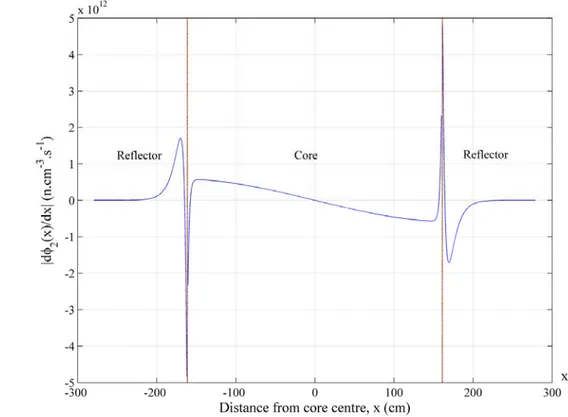
Calculations of ex-core neutron noise induced by in-core noise source or vibrating assembly were performed for a sample homogeneous reflected core in a 2-group 1-D model. The spatial vectors r and rp which refer to the induced noise and noise source positions in the above equations are denoted here by x and x , respectively in the 1-D p model. First, the static diffusion equations are solved for the neutron fluxes and the multiplication factor which later are used for determining the space-dependent noise. Figure 1 shows the space-dependent neutron fluxes in the fast and thermal groups of the investigated case. The spatial derivatives of the fluxes are presented in Figs 2 and 3. The figures show the discontinuity of the derivative of the flux at the core-reflector interface, representing the continuity of the current.
The calculation of the noise induced by vibrating materials, such as control rods or fuel assemblies, requires the calculation of the derivative of the Green’s function with respect to the noise source coordinate x , as shown by the right hand side of Eq. (13). p Since the solution of the direct equation for the Green’s function with CoreSim is not an analytical function of x an approximate numerical method is required. The fuel p, assembly vibration is modelled by shifting materials for a very fine mesh of about 3 mm at a specified assembly location. It means that here we have perturbations in all absorption, fission and removal cross-sections. Therefore, in the 2-group version of Eq. (13) there are three terms, corresponding to the three cross-section perturbations as seen on the r.h.s. of Eq. (1). Figures 4, 5 and 6 show an example of the magnitude and phase of the spatial derivatives of the Green’s function components corresponding to the absorption cross-section change. The ex-core detector position is specified at -188 cm, i.e. in the reflector. This is the closest how the signal of an ex-vessel detector can be simulated in a model with vacuum boundary conditions, assuming the vanishing the flux at the extrapolation length. It is seen that the derivative of the Green’s function w.r.t. the perturbation position is discontinuous at the detector position, but in practice only
p
x positions in the core that are of interest.
Figure 7 shows example results of the Green’s function itself, which is equivalent to the space-dependent noise induced by an absorber of variable strength, for two different
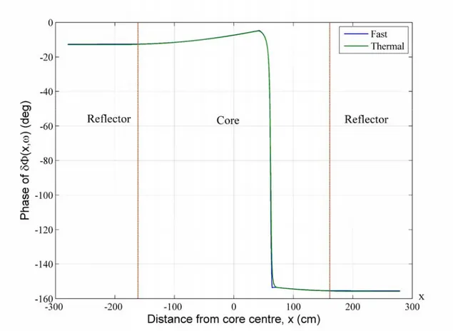
noise source positions. The magnitude and phase of the space-dependent noise induced by an assembly vibration is shown in Figs 8 and 9. The noise calculations are performed at the frequency of 8 Hz.
Fig. 1 Spatial distribution of the static neutron fluxes in the fast and thermal groups.
Fig. 2 Spatial derivative of the static fast flux.
Fig. 3 Spatial derivative of the static thermal flux.
Fig. 4 Magnitude of the spatial derivative of the Green’s function w.r.t. the perturbation position x in the fast group at an ex-core detector position (x = -188 cm). p
Fig. 5 Magnitude of the spatial derivative of the Green’s function w.r.t. the perturbation position x in the thermal group at an ex-core detector position (x = -188 cm). p
Fig. 6 Phase of the spatial derivative of the Green’s function w.r.t. the perturbation position xp in the fast and thermal groups at an ex-core detector position.
Fig. 7 Space-dependent thermal noise induced by an absorber of variable strength at two different in-core positions.
The amplitude and the phase of the fast and the thermal noise, induced by the vibration of a vibrating assembly, is shown in Figs 8 and 9, respectively, for a given equilibrium position of the assembly, as a function of the detector position in the core. In these calculations, the / dε model was used, such that two absorbers of variable strength with opposite phase, positioned at 43.3 and 64.7 cm, respectively, were used. This is only for illustration and in order to show similarity with analytical results obtained earlier for vibrating absorbers in 1-group theory (Pázsit 1977, 1978). The equilibrium position of the assembly (around which it performs the small amplitude vibrations) lies in the right half of the core (left from the core centre). Correspondingly, the amplitude of the noise is discontinuous at the rod position, and the amplitude is significantly smaller on the right hand side of the rod than on the left hand side. It is also interesting to observe that the noise amplitude is much larger in the fast group than in the thermal group. For a vibrating control rod, which corresponds to a thermal absorber, the amplitude of the noise would have been larger in the thermal group.
Fig. 8 Magnitude of the space-dependent thermal and fast noise induced by a vibrating assembly.
Fig. 9 Phase of the noises induced by a vibrating assembly.
1.4 Conclusions
The above calculations show that it is possible to calculate the effect of the vibrating fuel assembly by modelling the vibrations with a fine spatial resolution. The 1-D model has the potential to calculate the derivatives of the Green’s function with fine meshes without a memory problem, and therefore can be used to calculate simulate assembly vibrations. In the continuation of the work both the fine mesh and the adjoint method in 1-D and 2-D models will be used to simulate fuel assembly vibration.
In the 2-D model, if all meshes are as fine as realistic vibration strengths, the total number of meshes becomes very large which may cause memory overload problem. However, it is not needed to divide all fine meshes except the meshes around the edges of a vibrating assembly where the vibration is modelled by shifting materials by one mesh. In order to simulate the vibration of assembly at a flexible strength, CoreSim is continuously improved to be able to handle non-uniform mesh sizes with a flexible mesh size for the edges of vibrating assembly so that any vibration strength could be simulated. This improvement will be continued in the next stage, and used to calculate the change of the amplitude of the ex-core noise during the fuel cycle.
2 Extension of the traditional Rossi-alpha method to
two energy groups
2.1 Abstract
The traditional methods using higher moments of the detector counts, notably the Feynman- (variance to mean) and Rossi-alpha (temporal correlations) methods, are based on an energy-independent, or one-group, theory. The corresponding Feynman- and Rossi-alpha formulae were thus derived in a one-group theory setting. This energy-independent approach was experimentally justified since the methods appear to work well in a wide range of cases. The physical reason for this sufficiency is that until recently, the applications were mostly made in small thermal systems. In such systems, the thermal neutrons dominate in the system due to the fact that their lifetime is several orders of magnitude larger than the slowing down time, i.e. the lifetime of the fast neutrons. The influence of any possibly existing spectral effects is further diminished in small weakly reflected systems, where point kinetic behaviour dominates, and the spatial shape of the thermal and fast neutrons is identical. The result is that, if the delayed neutrons are disregarded, the temporal statistics of the detector counts is determined by one single parameter, the lifetime of the prompt neutron chain, and hence the Feynman- and Rossi-alpha formulae contain one single exponential.
However, there have been an increasing number of indications that in certain situations the traditional description may not work satisfactorily. From the experimental point of view, in several measurements it was found that the temporal behaviour of the Feynman- or Rossi-alpha measurements could not be fitted by one single exponential, rather two, or sometimes even more, exponential terms and corresponding exponentials were needed. The reasons for such behaviour can be manifold. One such case is that of fast reactor cores, including the Accelerator Driven Systems (ADS). In fast reactor cores, and in particular in those with a hard neutron spectrum, the dominance of the thermal neutrons is diminished, and the applicability of a one-group treatment far not obvious. Another case is that of the reflected systems, when the detector is placed close to, or in the reflector. Simply expressed, the die-away time of fast and thermal neutrons is rather different in the multiplying core and in the non-multiplying reflector, and this manifests itself in the fact that in such measurements, even with thermal cores, again two or more exponentials were found in the Rossi-alpha measurements.
The energy and spatial effects can be described by a full space-energy-dependent approach, such as in the original Pál-Bell equations, or in the later works of Munoz-Cobo et al (Pázsit and Pál, 2008). In such an approach, the existence of multiple alpha modes arises naturally by seeking the solution of the time-dependent problem with an expansion w.r.t. the eigenfunctions of the static equations. The problem is that this approach is rather non-transparent, and requires an assumption of the system configuration and the calculation of the corresponding eigenfunctions.
A far more pragmatic approach is to extend the theory of the Feynman- and Rossi-alpha methods to two energy groups, still in the same space-independent model as in the traditional works. With this extension, if one still disregards the delayed neutrons, the
temporal behaviour will be determined by two exponentials, and the whole theory still remains manageable fully analytically.
The usefulness of a two-group description for interpreting neutron die-away measurements in pulsed experiments has been known for quite some time in nuclear safeguards, at the deterministic level. The corresponding method is called the differential die-away analysis (DDAA). This technique is usually applied for the detection of special nuclear materials (i.e. fissile material) embedded in a hydrogenous surroundings, carried in transportable cargoes (Kunz, Caldell and Atencuo, 1982; Croft, Mc Elroy, Bourva and Villani, 2003; Jordan, 2006; Jordan and Gozani, 2007; Jordan, Gozani and Vujic, 2008). The essence is that a pulse of fast neutrons is injected into a large hydrogenous medium which contains a given quantity of fissile material. The initial fast neutrons decay quickly, by slowing down during a relatively short time and becoming thermal, as well as they leak out and get absorbed. This behaviour gives rise to a fast decaying exponential. One part of the slowed down, thermal neutrons causes fissions while the rest leaks out of gets absorbed. These thermal fissions give rise to the appearance of further fast neutrons, whose away time will be determined by the die-away of the thermal neutrons (since they constitute the source of these neutrons). Due to the relatively long lifetime of the thermal neutrons, a second, slowly decaying exponential will also be present in the die-away of the fast neutrons. By using a detector which counts only the neutrons above the cadmium cut-off, one obtains a definite indication about the presence of fissile material in the medium. Namely, without the presence of fissile material, there would only be one (fast) exponential. If fissile material is present, the die-away (the number of counts vs. time) curve can be approximated by a sum of two exponentially decreasing functions.
The motivation for the present work came from a recent suggestion to extend the traditional DDAA method, which is a deterministic method whose application requires the use of a pulsed neutron generator, to the stochastic case. It was suggested that similarly to the case of reactivity measurement methods, where pulsed measurements can be replaced by the measurement of temporal correlations (Rossi-alpha method) with a stationary random source, the DDAA method can also be converted into a type of Rossi-alpha measurement of fast neutrons, where the pulsed source can be replaced by the inherent source of neutrons (spontaneous fissions) in the sample (Menlove et al, 2009). The method was called the differential die-away self-interrogation (DDSI) technique. In Menlove et al (2009), it was assumed that the dependence of the temporal correlations of the detector counts of fast neutrons at two different time points has the same dependence on the time lag τ as that of the detector counts at time t in the traditional DDAA method with an interrogating pulse emitted at t=0 . However, in the above work, the DDSI formula was not derived from first principles, only its form was assumed by analogy to the deterministic case. Such an empirical formula can identify the exponents, but not the corresponding coefficients, since they depend on the second moments of the number of neutrons per fission, which is not present in the deterministic DDAA formula, which only contains first moment quantities.
Obviously, the DDSI formula is equivalent to the two-group version of the Rossi-alpha formula. For the reasons described in above, a two-group version of the Feynman- and Rossi-alpha formulae would be useful also for reactivity measurements in fast reflected cores. We have therefore decided to elaborate the theory of neutron fluctuations, more concretely that of the Feynman- and Rossi-alpha formulae, in a two group approach
with the master equation technique. Preliminary results were already obtained (Pál and Pázsit, 2011). Here we give the basics of the theory of the two-group version of the Rossi-alpha formula, with the first results. The calculations for the Rossi-alpha formula show that the temporal dependence of the detection rate of fast neutrons at time t +τ, following a triggering detection at time t indeed has a form of the sum of two exponentials, just as in the traditional DDAA method, but the coefficients of the two terms are different. The correct form of the two-group Rossi-alpha formula is given and some possible further applications of the method are discussed.
2.2 A simple stochastic model
Assume that two types of neutrons can be found in the medium. One of them with energy above a well defined cut-off is denoted as group # 1, indicated by subscript “1” (fast neutrons), while the other one with energy not larger than the cutoff, by group # 2, indicated by subscript “2” (thermal neutrons). Let n1( )t and n2( )t be the random numbers of the fast and the thermal neutrons, respectively, in a medium at time instant
0
t ≥ , provided that at time moment t=0 there was either one fast or one thermal
neutron in the medium.
The statistical treatment of neutron counts is based on using master equations for the probability distributions of the neutrons in the system, and on the moments of the detector counts. The method can be illustrated by first developing the one-time (“one-point”) distributions for the probabilities of finding a given number of fast and thermal neutrons in the system, when the process was started by one single neutron. Thus we define the probabilities
{
n1( )t =n1, ( )n2 t =n S2 | j}
=p n n t S( , , |1 2 j), j =1,2, P (14) where{
}
{
}
1 1(0) 1, (0)2 0 and 2 1(0) 0, (0)2 1 S = n = n = S = n = n = , (15)that n1 fast and n2 thermal neutrons can be found in the medium at the time instant 0
t ≥ , provided that at the time instant t=0 there was only either one fast neutron or
one thermal neutron in the medium. Here, S1 stands for a starting fast neutron, whereas
2
S stands for a thermal source neutron.
In order to derive the master equations, one needs the intensities of the various processes the neutrons can undergo. Hence we define the total reaction intensity
1 1a R
λ =λ +λ
of the fast neutrons, where λ1a and λR are the intensities of the absorption and thermalization (“removal”) of fast neutrons, respectively. In reactor physics terminology, these are given as λ = Σ1a v1 a1, where v1 stands for the velocity of the fast neutrons, and
1 a
Σ is the macroscopic absorption cross section of the fast neutrons. Similar expressions exist for the other intensities. The intensities of the thermal neutron processes are defined as
2 2a 2f
λ =λ +λ
Here, λ2a is the intensity of the capture of thermal neutrons, while λ is the intensity of 2 f the fission caused by thermal neutrons. Further, f ki( ) will denote the probability that exactly k fast neutrons are produced in an induced thermal fission event. Fast fissions will be neglected in the present treatment.
It is worth noting that since we are going to use the backward equations, which operate on the source co-ordinates only, it would be possible to write down equations which only describe the evolution of the probability distribution of the fast neutrons, irrespective of the number of thermal neutrons in the system. We will use this property of the backward equation when determining the two-time (“two-point”) distributions of the detected neutrons in the fast group (the “fast Rossi-alpha formula”).
2.2.1 Backward Kolmogorov equations
From obvious considerations, the integral form of the backward Kolmogorov equations determining the probabilities p n n t S( , , |1 2 1) and p n n t S( , , |1 2 2), respectively, can be written down as 1 2 1 ( , , | ) p n n t S = 1 1 1 1 2 1 2 ( ) ( ) ,1 ,0 1 0 ,0 ,0 0 ( , , |1 2 2) , t t t t t t t n n a n n R e−λ δ δ +λ
∫
e−λ −′ dt′δ δ +λ∫
e−λ −′ p n n t S dt′ ′ (16) and 2 2 1 2 1 2 ( ) 1 2 2 ,0 ,1 2 0 ,0 ,0 ( , , | ) t n n a t t t n n p n n t S =e−λ δ δ +λ∫
e−λ −′ dt′δ δ + 2 1 1 1 2 ( ) 2 0 1 1 0 ( ) ( , , | ) , k k k t t t f i u u n v v n j j j k e λ f k p u v t S dt λ − −′ ∞ + + = + + = = = ′ ′∑
∑
∑
∏
∫
" " (17)Introducing the generating functions
1 2 1 2 1 2 1 2 1 2 0 0 ( , , | ) ( , , | ) n n , 1,2, j j n n g z z t S ∞ ∞ p n n t S z z j = = =
∑ ∑
= (18)from (16) and (17) one obtains for these the equations
1 2 1 ( , , | ) g z z t S = 1 1( ) 1( ) 1 1 0 0 ( , , |1 2 2) t t t t t t t a R e−λ z +λ
∫
e−λ −′ dt′+λ∫
e−λ −′ g z z t S dt′ ′ (19) and 1 2 2 ( , , | ) g z z t S = 2 2( ) 2( ) 2 2 0 2 0 ( , , | )1 2 1 , t t t t t t t a f e−λ z +λ∫
e−λ −′ dt′+λ∫
e−λ −′ q g z z t S dt⎡⎢⎣ ′ ⎤⎥⎦ ′ (20) SSM 2011:29respectively, where the generating function q(z) of the fission number multiplicity was introduced as 0 ( ) ( ) .k i k q z ∞ f k z = =
∑
(21)From these equations the various moments of the fast and thermal neutrons in the system can be derived. At first we will restrict the calculations only to the first moment. For the expectation of the number of fast neutrons in the system, when the process was started by one fast neutron, the results are analogous to the traditional DDAA measurement.
2.2.2 Calculation of the expectation of the number of fast neutrons.
Introduce the notations
1 2 1 2 1 1 1 1 1 ( , , | ) ( | ) z z g z z t S n t S z = = ⎡∂ ⎤ ⎢ ⎥ = ⎢⎢ ∂ ⎥⎥ ⎣ ⎦ (22) and 1 2 1 2 2 1 2 1 1 ( , , | ) ( | ) , z z g z z t S n t S z = = ⎡∂ ⎤ ⎢ ⎥ = ⎢⎢ ∂ ⎥⎥ ⎣ ⎦ (23)
for the expectations of the fast neutrons in the system at time t when the process was started by one fast and one thermal neutron injected at time t=0 , respectively. From equations (19) and (20) one obtains that
1 1( ) 1( | )1 0 1( | 2) , t t t t R n t S =e−λ +λ
∫
e−λ −′ n t S dt′ ′ (24) with 2( ) 1( | 2) 2 1 0 1( | )1 , t t t f n t S =λ q∫
e−λ −′ n t S dt′ (25) and 1 1 1 ( ) i z dq z q dz = ν ⎡ ⎤ ⎢ ⎥ = ⎢ ⎥ ≡ ⎣ ⎦ (26)where the subscript i stands for “induced”. For the Laplace transforms of n t S1( | 1) and
1( | 2) n t S one obtains 2 1 1 1 2 1 2 ( | ) ( )( ) R f LT s S s s n s q λ λ λ λ λ + = + + − (27) and 1 2 1 2 1 2 1 2 ( | ) . ( )( ) f R f LT q n s S s s q λ λ λ λ λ = + + − (28) SSM 2011:29
The two roots of the denominator are given by
(
)
(
)
2 1 1 1 2 1 2 1 2 1 1 4 2 2 eff s = −ω = − λ +λ + λ −λ + λ λ ν (29) and(
)
(
)
2 2 2 1 2 1 2 1 2 1 1 4 , 2 2 eff s = −ω = − λ +λ − λ −λ + λ λ ν (30) where 2 1 1 2 . R f eff i λ λ ν ν λ λ = (31)It is important to note that
2 0
ω >
and
1 2.
ω <ω
If νeff = , then 1 ω =1 0, i.e. the system is critical.
By using expressions (29) and (30) and performing the inverse Laplace transform, one obtains for the expectation of the number of fast neutrons, induced by one starting fast neutron, the result
2 1 2 2 2 1 1 1 2 1 2 1 ( | ) t t. n t S ω λ e ω λ ω e ω ω ω ω ω − − − − = + − − (32)
Similarly, the expectation of the number of fast neutrons, induced by one starting thermal neutron, is given by
(
1 2)
2 1 2 1 2 1 ( | ) f t t . n t S q λ e ω e ω ω ω − − = − − (33) SSM 2011:29Fig. 10 Expectation of the mean number of fast neutrons versus time.
As the results show, the time dependence of the expectation of the number of fast neutrons is described by the sum of two exponentials. Fig. 10 shows this expectation for the case when the process was started by one fast neutron. Since the expectation of the count rate of the fast neutrons is proportional to the mean number of fast neutrons at a given time in the medium, the curve in Fig. 10 can be regarded as being analogous to the time dependence of the mean count rate scaled to unity at the time moment t=0 . For completeness, although it will not be needed in the continuation, we list here the expectations of the number of thermal neutrons in the system, generated either one fast or one thermal initial neutron. With obvious notations, these are given as
(
1 2)
2 1 2 1 ( | ) R t t n t S λ e ω e ω ω ω − − = − − (34) and 2 1 2 1 1 1 2 2 2 1 2 1 ( | ) t t. n t S ω λ e ω λ ω e ω ω ω ω ω − − − − = + − − (35)2.3 Time correlation neutron counting with triggering on the
spontaneous fission events - the Rossi-alpha formula in two
groups
We turn now to the derivation of the Rossi-alpha formula in two energy groups. In this method the inherent source neutrons in the sample arising from the spontaneous fissions
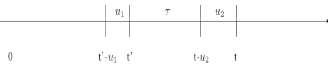
Fig. 11 Arrangement of the mutually non-overlapping time intervals t′ = −t u2−τ
are used for triggering the time correlation counting of the fast neutrons produced by the induced fissions in the sample.
From now on, we will only consider the fast neutrons in the system. Compared to the previous Section, the following extensions need to be made. Instead of one starting neutron, the neutron population in the sample will be induced by a stationary compound Poisson source, represented by the spontaneous fission source in the sample. This source will have an intensity s0 and number distribution of spontaneous fission neutrons f ks( ). We will consider a detector, and characterise the detector with the intensity of the detection of a fast neutron, λd. For obvious reasons, with the inclusion of a detector, we have to re-define the total reaction intensity of fast neutrons as
1 1a R d
λ =λ +λ +λ
Further, instead of one time instant, we will consider a two-time distribution, around t' and t , and seek the quantities N(t′−u t1, )′ and N(t−u t2, ), which are the numbers of detected neutrons in the time intervals ( '- , ')t u t1 and ( - , )t u2 t , respectively, where
2
t′ = −t u −τ. It is assumed that at a hypothetical time instant t=0 there are no free neutron in the assay sample, hence in the above, obviously t > 0. Here, τ is the time interval which separates the counting intervals u2 and u1. The indices “1” and “2” here refer to the first and second time instant, and not the energy group of the neutrons. Fig. 11 illustrates the time axis which helps to follow the further considerations.
Define the probability
{
}
( ) 1 1 2 2 1 2 1 2 1 2 (t′−u t, )′ =n, (t−u t, )=n | = 0, =0 =P D( , , , , , )n n t τ u u N N n n P (36) that the numbers of the detected fast neutrons in the time intervals ( '- , ')t u t1 and2
( - , )t u t are n1 and n2, respectively, provided that at the time instant t = there was 0 no free neutron in the system. By using the same methodology as in Pázsit and Pál (2008) on p. 59, one can obtain for the logarithm of the generating function
1 2 2 1 ( ) ( ) 1 2 1 2 1 2 1 2 1 2 0 0 ( , , , , , ) ( , , , , , ) n n D D n n z z t τu u ∞ ∞ P n n t τ u u z z = = =
∑ ∑
G (37)the following expression:
{
}
( ) 1 2 1 2 0 0 1 2 1 2 1 ln D( , , , , , )z z t τu u =s t r g z z v⎡ ( , , , , ,τ u u S| )⎤−1 dv, ⎢ ⎥ ⎣ ⎦∫
G (38)where s0 is the intensity of the spontaneous fission events, and
0 ( ) ( ) k s k r z ∞ f k z = =
∑
(39)is the generating function of the probability f ks( ) that the number of fast neutrons in a spontaneous fission event is exactly k .
The key part of (39) is the generating function
1 1 2 2 1 2 1 2 1 1 2 1 2 1 1 2 0 0 ( , , , , , | ) ( , , , , , | ) n n, n n g z z t τ u u S ∞ ∞ p n n t τ u u S z z = = =
∑ ∑
(40)where p n n t( , , , , ,1 2 τ u u1 2 |S1) is the probability that the numbers of the detected fast neutrons in the time intervals ( '- , ')t u t1 and ( - , )t u2 t are n1 and n2, respectively, provided that at the time instant t = there was one fast neutron in the system. 0 Obviously, the next step is to write down the two-group backward Kolmogorov equations. One obtains that
1 1 1 2 1 2 ( ) 1 2 1 2 1 ,0 ,0 1 0 ,0 ,0 ( , , , , , | ) t t t v n n a n n p n n t τ u u S =e−λ δ δ +λ e−λ − δ δ dv+
∫
1( ) 1 2 1 2 0 ( , , , , , ) t t v d e A n n v u u dv λ λ − − τ +∫
1( ) 1 2 1 2 2 0 ( , , , , , | ) , t t v R e p n n v u u S dv λ λ − − τ∫
(41) where 1 2 1 2 ( , , , , , ) A n n v τ u u = 1 2 1 2 2 1 ,0 ,0 2 2 1 ,1 ,0 (v u τ u)δn δn (v u τ) (u τ u v)δn δn Δ − − − + Δ − − Δ + + − + 1 2 1 2 2 2 ,0 ,0 2 ,0 ,1 (v u ) (τ u v)δn δn ( ) (v u v)δn δn , Δ − Δ + − + Δ Δ − (42)and p n n t( , , , , ,1 2 τ u u S1 2 | )2 is the probability that the numbers of the detected fast neutrons in the time intervals ( '- , ')t u t1 and ( - , )t u2 t are n1 and n2, respectively, provided that at the time instant t = there was one thermal neutron in the system. It 0 can be shown that the probability p n n t( , , , , ,1 2 τ u u S1 2 | )2 satisfies the following integral equation:
2 2 1 2 1 2 ( ) 1 2 1 2 2 ,0 ,0 2 0 ,0 ,0 ( , , , , , | ) t n n a t t v n n p n n t τ u u S =e−λ δ δ +λ e−λ − δ δ dv+
∫
2( ) ( ) 2 0 1 2 1 2 1 0 ( ) ( , , , , , | ) , t t v k f i k e λ f k b n n v u u S dv λ − − ∞ τ =∑
∫
(43) where ( ) 1 2 1 2 1 ( , , , , , | ) k b n n v τ u u S = 11 1 1 21 2 2 1 2 1 2 1 1 ( , , , , , | ). k k k n n n n n n j j j p n n v τ u u S + + = + + = =∑
"∑
"∏
(44)Introducing the generating function
1 2 1 2 1 2 1 2 2 0 0 1 2 1 2 2 1 2 ( , , , , , | ) n n ( , , , , , | ) n n , g z z t τ u u S ∞ ∞ p n n t τ u u S z z = = =
∑ ∑
(45)and taking into account (40), one can obtain the following generating function equations: 1 2 1 2 1 ( , , , , , | ) g z z t τ u u S = 1 1( ) 1( ) 1 0 0 ( , , , , , )1 2 1 2 t t t t v t v a d e−λ +λ
∫
e−λ − dv+λ∫
e−λ − B z z v τ u u dv+ 1( ) 1 2 1 2 2 0 ( , , , , , | ) , t t v R e g z z v u u S dv λ λ − − τ∫
(46) and 1 2 1 2 2 ( , , , , , | ) g z z t τ u u S = 2 2( ) 2( ) 2 0 2 0 ( , , , , ,1 2 1 2 | )1 , t t t t v t v a f e−λ +λ e−λ − dv+λ e−λ − q g z z v⎡ τ u u S dv⎤ ⎢ ⎥ ⎣ ⎦∫
∫
(47) where 1 2 1 2 ( , , , , , ) B z z v τ u u = 2 1 2 1 2 2 1+ Δ −⎢⎡⎣ (v u − −τ u )− Δ −(v u −τ) (1⎦⎤⎥ −z )+ Δ −⎡⎣⎢ (v u )− Δ( ) (1v ⎥⎤⎦ −z ). (48) By using the procedure described in Pázsit and Pál (2008) pp. 85-86, one can prove the statement that the generating function G( )D( , , , , , )z z t1 2 τ u u1 2 is asymptotically stationary, i.e. the limit( ) ( )
1 2 1 2 1 2 1 2
lim D( , , , , , ) D ( , , , , )
st
t→∞G z z t τ u u =G z z τ u u (49)
exists. In order to derive the stationary probability that a fast neutron detection takes places in the time interval dτ =du2, provided that a spontaneous fission neutron was detected exactly τ time earlier, one needs the stationary covariance function of the detected fast neutrons
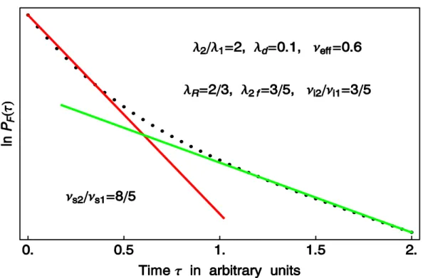
Fig. 12 Dependence of the intensity P τF( ) on the time τ at given values of the model parameters. 1 2 2 ( ) ( ) 1 2 1 2 1 2 1 2 1 ln ( , , , , ) ( , , ) D D st st z z z z u u u u z z τ τ = = ⎡∂ ⎤ ⎢ ⎥ = ⎢ ∂ ∂ ⎥ ⎢ ⎥ ⎣ ⎦ R G (50)
and the stationary expectation of the detected fast neutrons, Mst( )D( )u . The fast neutron 1 Rossi-alpha formula is defined by considering the expression PF( )τ τd +o d( )τ of detecting a fast neutron in the time interval d τ provided that a spontaneous fission neutron was detected exactly τ time earlier. With the help of the above quantities, this can be expressed by ( ) 1 ( ) 1 ( , , ) ( ) ( ) . ( ) D st F D st du d P d o d M du τ τ τ τ+ τ = R (51)
Determination of P τF( ) requires the evaluation of (50) as well as determination of
( ) 1
( )
D st
M u and using a first term series expansion for infinitesimal values of du1 and
2
du =dτ. The calculation is straightforward, but very extensive. The details of the calculations are not given here, they can be found in Pál and Pázsit (2011). Here we only give the final result, which has the form
2 2 2 1 2 1 1 ( ) 2 R f s F d i s P τ τd λ ν λ λ ν ω ω ν ⎛ ⎞⎟ ⎜ ⎟ ⎜ = ⎜⎜ + ⎟⎟× ⎟⎟ ⎜⎝ ⎠
(
)
1 2 2 1 1 2 1 1 1 2 2 2 2 2 2 2 1 ( )( ) ( )( ) . e e d ω τ ω τ ω λ ω λ ω ω λ ω λ ω τ λ ω ω − − − + − − + − (52)Here, r1 =νs1 is the mean number of fast neutrons originating from a single spontaneous fission, while r2 =νs2 is the second factorial moment of the same number. The dependence of P τF( ) on τ is shown in Fig. 12 with selected values of model parameters.
2.4 Discussion and conclusions
Eq. (52) shows that the two-group Rossi-alpha formula consists indeed of two exponentials with the same exponents as the conventional DDAA formula. Hence in this respect the conjecture of Menlove et al (2009) is correct. However, from such an empirical extension of the one-point expectations to the two-point joint conditional probability, there is no possibility to give the correct coefficients of the exponents. Partly, this is because being a second moment expression, the DDSI formula contains the second factorial moments of the number of neutrons generated in both spontaneous and induced (thermal) fission. These factors do not appear in the DDAA formula, which corresponds to a completely different physical situation. Application of the DDSI method in cases when not only the exponents, but also the coefficients of the two terms are of interest, has therefore be based on the correct formula (52).
In this paper only the “fast neutron Rossi-alpha” formula, corresponding to the DDSI method as suggested in Menlove et al (2009), was calculated. It is based on the detection intensity of fast neutrons at time τ , provided that a fast neutron was detected at time t=0 . However, the present treatment opens up the possibility of calculating “thermal” and “mixed” Rossi-alpha expressions as well, based on the detection intensity of either fast or thermal neutrons at time τ , provided that one fast or one thermal neutron was detected at time t=0 . Although the time dependence will be determined in all cases by the same to exponents, the relative weight of these terms will be different in the different expressions, making it possible to determine more parameters of the system. Another piece of further work will be the calculation of the two-group version of the Feynman-alpha formula.