Quantification of temporal changes in
metal loads – Moss data over 20 years
Joseph Addai
Master’s of Science Thesis in Geoinformatics
TRITA-GIT EX 07-003
School of Architecture and the Built Environment
Royal Institute of Technology (KTH)
100 44 Stockholm, Sweden
March 2007
TRITA-GIT EX 07-003 ISSN 1653-5227
Dedicated to my Mum and Dad
Who over the years have taught me that with a willing heart and mind
everything is possible.
ABSTRACT
Environmental monitoring, assessment and conservation programmes worldwide have led to the development of scientific and technological methods to study the changes in our environment. As a result, a technique for monitoring atmospheric metal deposition was developed in Sweden in the 1960s. This technique is based on the principle that, carpet-forming moss obtains its nutrients from dry deposition particles in the air. The Swedish Environmental Research institute (IVL) has a database of concentrations of metals in terrestrial mosses. These were sampled during the national moss surveys (1975 – 2000). From these point data, long-term changes in the deposition loads can be studied.
One aim of this project is to create continuous surfaces for these point data and to develop a technique to map the spatio-temporal changes. It also seeks to quantify the temporal changes in metal loads of the moss data for over 20 years. With the amount of data increasing from various air quality assessments and monitoring methods, it is prudent to approach the data analysis from a multidisciplinary perspective. By using statistics, geostatistic, GIS and visualization methods, the quantitative, spatial and temporal trends of the moss surveys were analysed. Multidimensional visualizations based on exploratory data analysis were applied to the data to visualize and reveal trends in the multivariate data.
The project area comprised the whole Sweden with the data from 1975 to 2000, with the exception of the moss survey in 1975, which was conducted only in southern Sweden. A combination of GIS, geostatistics and high dimensional visualization techniques were applied in the data cleaning and analysis stages.
The results of the project show the rate of change of metal loads over the years and the spatial distribution of the metal depositions as well. The visual approach used from the data cleaning to results presentation makes it easily comprehensible to non-scientist as well.
ACKNOWLEDGEMENTS
It was by chance I found this thesis online, but it was by choice that I decided to undertake it with all the uncertainties and challenges. I could not have done it all by myself. Therefore I would like to express my sincere gratitude to my supervisor Katrin Grünfeld, PhD., for her constant support, critique and advice, my examiner Prof. Yifang Ban for her advice and guidance and to all the staff of the Geodesy and Geoinformatics Department of KTH. To Huaan Fan, PhD., and Solvieg Winell, thanks a lot for your lovely welcoming smiles.
I am forever indebted to my family for their constant support, love and guidance through all these years of my studies at home and abroad. To Nana Joseph Gyamfi and his family, I am very grateful for providing me with a home throughout my stay in Stockholm, Sweden.
To my family and friends at the student group of St Eugenia Catholic Church, I can never thank you enough but you will always be in my heart and prayers. Fr. Klaus thanks a lot for providing a place we could offload all our fears, pain and anxiety and load the strength to face each new week. To Michelle Andersson, I am grateful you always got me back on my feet whenever I was down.
During my studies at KTH, I have in diverse ways collaborated with a host of student from all over the world and I wish to extend my sincere appreciation to all of you for your company. Ultimately, to the many wonderful people who made my time in Sweden truly exceptional. Many thanks to you all.
Stockholm, Sweden, December 2006 Joseph Yaw Addai
TABLE OF CONTENTS
Page
Abstract iii
Acknowledgements v
Table of contents vii
List of Tables ix List of Figures x List of Appendices xi CHAPTER 1: INTRODUCTION 1.1 Background 1 1.2 Literature Review 2 CHARPTER 2: AIM 2 CHAPTER 3: DATA 3.1 Moss Sampling Technique 3
CHARPTER 4: METHODS 4.1 Exploratory Data Analysis 9
4.1.1 Parallel Coordinate Plot 9
4.1.2 Scatter Plot 10
4.2 Geographic Information Systems 11
4.2.1 Visual Data Analysis 12
4.2.2 Spatial Interpolation 12
4.3 Quantification of Trends 14
CHARPTER 5: RESULTS AND DISCUSSION 5.1 Data Cleaning 15 5.2 Data Exploration 17 5.3 Spatial Interpolation 20 5.4 Spatial Trends 24 5.5 Temporal trends 25 CHARPTER 6: CONCLUSIONS AND RECOMMENDATIONS 6.1 Conclusions 29 6.2 Recommendations 30 REFERENCES 33 APPENDICES Appendix A - E 35 Appendix F – G 50 Appendix H – M 53 Appendix N 64 vii
LIST OF TABLES
Table 3.1. Summary of sample count of moss survey (1975 – 2000). 8
Table 3.2. Statistical summary of raw moss data (1975 – 2000). 8
Table 4.1. Relative scale to quantify pollution loads (mg/kg dw). 15
Table 5.1. Summary of sample count of clean moss data (1975 – 2000). 16
Table 5.2. Statistical summary of cleaned moss data (1975 – 2000). 16
Table 5.3. Summary of median of deposition values from spatial interpolation 21
results. Table 5.4. Summary of mean deposition values from spatial interpolation results. 21
Table 5.5. Year-to-year rate of change of deposition (based on median values). 25
Table 5.6. Year-to-year rate of deposition for northern Sweden. 26
Table 5.7. Year-to-year rate of deposition for mid Sweden. 28
Table 5.8. Year-to-year rate of deposition for southern Sweden. 28
LIST OF FIGURES
Figure 1.1. Some sources of air pollution. 1
Figure 3.1. Map of moss survey (1975). 5
Figure 3.2. Map of moss survey (1980). 5
Figure 3.3. Map of moss survey (1985). 6
Figure 3.4. Map of moss survey (1990). 6
Figure 3.5. Map of moss survey (1995). 7
Figure 3.6. Map of moss survey (2000). 7
Figure 4.1. Example of a parallel coordinate plot - moss survey 1975 – 2000. 10
Figure 4.2. Example of a scatter plot - moss survey 1975 – 2000. 11
Figure 4.3. Example of a box plot (zinc, year 1980). 12
Figure 4.4. Example of a histogram (zinc, year 1980). 13
Figure 5.1. Histogram of clean zinc data (2000). 17
Figure 5.2. Scatter plot (left) and Parallel coordinate plot (right) of moss data. 18
Figure 5.3. Scatterplot (left) and parallel coordinate plot (right) showing the 18
position of trend of north eastern tip of Sweden. Figure 5.4. Parallel coordinate plot (left) and scatterplot (right) showing 19
pollution load of Northern Sweden (1975 – 2000). Figure 5.5. Parallel coordinate plot (left) and scatterplot (right) showing 19
pollution load of Southern Sweden (1975 – 2000). Figure 5.6. Interpolated maps of copper and nickel deposition (2000). 20
Figure 5.7. Maps of copper and nickel deposition loads (2000). 21
Figure 5.8. Scatter plot of cross validation results for lead 1985. 22
Figure 5.9. Scatter plot of cross validation results for lead 1995. 23
Figure 5.10. Scatter plot of cross validation results for vanadium 1990. 24
Figure 5.11. A graph of rate of change of deposition (based on median values). 26
Figure 5.12. Changes in pollution loads (1975 – 2000). 27
Figure 5.13. Bar chart of deposition rate for northern Sweden. 27
Figure 5.14. Bar chart of deposition rate for mid Sweden. 28
LIST OF APPENDICES
Appendix A Deposition map of copper (1975 – 2000) 35
Appendix B Deposition map of nickel (1975 – 2000) 38
Appendix C Deposition map of lead (1975 – 2000) 41
Appendix D Deposition map of vanadium (1975 – 2000) 44
Appendix E Deposition map of zinc (1975 – 2000) 47
Appendix F Sample histograms of raw and clean moss data 51
Appendix G Sample box plots of moss data 52
Appendix H Deposition maps of copper (1975 – 2000) from IVL website 53
Appendix J Deposition maps of nickel (1975 – 2000) from IVL website 56
Appendix K Deposition maps of lead (1975 – 2000) from IVL website 59
Appendix L Deposition maps of vanadium (1975 – 2000) from IVL website 62
Appendix M Deposition maps of zinc (1975 – 2000) from IVL website 65
Appendix N Statistical summary of interpolation results 68
CHAPTER ONE: INTRODUCTION 1.1 Background
“We are astronauts—all of us. We ride a spaceship called Earth on its endless journey around the sun. This ship of ours is blessed with life-support systems so ingenious that they are self-renewing, so massive that they can supply the needs of billions. However for centuries we have taken them for granted, considering their capacity limitless. At last we have begun to monitor the systems, and the findings are deeply disturbing.
Scientists and government officials of the United States and other countries agree that we are in trouble. Unless we stop abusing our vital life-support systems, they will fail. We must maintain them, or pay the penalty. The penalty is death” (Young, 1970).
Figure. 1.1. Some sources of air pollution (Batelle, 2006; Berkeley Lab, 2006).
For ages, humans have sort to make maximum use of every available resource in nature. This on the positive side has brought a lot of benefits but on the contrary, has caused great destruction to our planet. Air pollution, addition of harmful substances to the atmosphere has huge impact on the environment which invariably affects human health and quality of life. Since the advent of pollution controls and standards, scientists have measured the amount of pollution and their sources.
Metals are emitted into the atmosphere from many sources – metallurgical, combustion, traffic and other processes (Fig. 1.1). These heavy metals are released as complex particles, metal fragments, as primary oxides or salts of a variety of acids, but may also (mainly mercury) be emitted in gaseous form. Upon their release, these metal species change gradually. The metals’ toxicity, mobility, and other properties are determined by the interaction between the metal properties and the local environment. The bulk of the emission from any point source is often transported to remote areas, this distance between emission point source and deposition sites depends on a number of factors among which are, size, surface structure and density of metal particles, position and height above ground of the emission point, local ventilation climate, and topography. The assessment of metal deposition to vegetation may be done by a variety of techniques. It should be emphasised that, no single method is the best. The major problems with most methods is that they are time demanding and expensive
1.2 Literature Review
Since the development of a new technique to assess metal deposition in Sweden in the 1960 (Rühling & Tyler, 1968; Tyler, 1970), there have been a lot of studies in this direction all over Europe. The measuring techniques are essentially the same but the method has been applied in different places at different times.
In the study of Rühling & Tyler, (2001) on the changes in atmospheric deposition rate of heavy metals (1969/70 – 1995), a comparison of moss and direct deposition measurements were compared. Interestingly, the results showed no difference in the uptake of some elements by moss or directly measured deposition at many stations in Denmark, Norway and Sweden. The correlation was almost perfect!!! This however, has not been the case for the Norwegian and some other studies. From those studies, moss carpets from extreme coastal stations had lower concentrations of several elements (e.g., Ni, and Zn) than expected from the overall moss. This was thought to be the exchange site competition with cations in marine salts deposited in excess in exposed coastal areas. From this same study, the influence of local, national and foreign emissions was reflected by the higher deposition of heavy metals in southern Sweden than the northern part of Sweden. The effects of air quality improvement, improved emission control in new and existing industries and fossil fuel stations as well as other environmentally friendly measures were evident in the significant reduction of pollution loads recorded over the years. Johansson et al. (2001) look at the impact of atmospheric long-range transport of lead, mercury and cadmium on the Swedish forest environment. They estimate that, about 80 % of the atmospheric depositions of these metals in southern Sweden are emissions of foreign origin. During the 20th century mainly, there has been a considerable increase in the mor layer of the forest soils of these three elements. However, the atmospheric deposition of the metals has declined during the most recent decades. The accumulation factors of mercury and lead in the forest top soils are already above the levels at which adverse effects on soil biological processes and organisms have been demonstrated. This is an apparent risk of lead induced reduction in microbial activity over southern part of Sweden.
It is important to note however that almost all the moss sampling surveys conducted in Sweden, Scandinavia and Europe at large, present positive results of a reduction in atmospheric deposition of metal loads.
CHAPTER TWO: AIM
The aim of this thesis is to quantify the temporal changes in the metal loads – moss data for over 20 years. This will involve multi – element pattern analysis, spatial trends and finally the temporal variations over the years. These results will communicate effectively across the various strata of society and not only comprehensible to scientist.
CHAPTER THREE: DATA 3.1 Moss Sampling Technique
A new technique for assessing atmospheric metal deposition was developed in Sweden in the 1960’s (Rühling & Tyler, 1968; Tyler, 1970). This technique was based on the principle that carpet-forming bryophytes (pleurocarp mosses) obtain their mineral nutrition mainly from rain, melting snow and dry deposition of particles in the air. These mosses are not rooted in their subtrate and any uptake of elements, including heavy metals from the soil is very negligible (Tamm, 1953). New biomass develops from old and usually remains viable for about three years, depending on the moss species. During this period the tissue accumulates and integrates heavy metal deposition very efficiently. The almost complete absence of a cuticle or an epidermal layer of leaves implies that numerous cation exchange sites in the cell walls are exposed to the ambient atmosphere and are capable of absorbing metal ions with a high affinity for such sites. Also, their large surface area and other structural properties promote a mechanical retention of deposition minerals, therefore leaching from the tissues are very small or negligible. The availability of moss in most geographic locations has facilitated its use in monitoring heavy metal deposition in many countries around the globe. A nationwide survey has been carried out in Sweden every five years since 1968/1970, in Norway since 1976/1977 (Steinnes, 1980), in all Nordic countries since 1980 (e.g. Gydesen et al., 1983) and also in a form of joint programme in many European countries since 1990 (Rühling, 1994). Two moss species, Hylocomium splendens and Pleurozium schreberi, have been used in the surveys. Both are wide spread, carpet-forming species, abundant in coniferous and mixed forest throughout northern Europe. Pleurozium is characterised by bi- or tripinnate sympodia with a clear separation of each annual growth. For practical reasons, pleuzorium was preferred in most cases.
Sampling was performed mainly during the summer months, though season has proven to have very little influence on heavy metal concentrations in moss (Berg & Steinnes, 1997). In areas of anticipated high deposition rate of heavy metals a denser sampling grid was used and areas of known pollution sources were avoided. All sampling sites were located at least 300 m from main roads and built up areas and at least 100m away from any road or single building. At each site 5 - 10 sub samples were taken within a 50 x 50 m area and combined to one collective sample. They were collected in small gaps in the forest or in a young plantation, not directly exposed to through fall precipitation.
Sampling and sample handling were carried out using chemically inert plastic gloves and bags. They were then stored in a refrigerator or dried and stored deep-frozen until further treatment. The reference materials were taken through all routines to control the effects of subsequent sample treatments and procedures. Generally, samples were pre-treated for analysis according to the following scheme. The three youngest fully developed segments of each sympodium of Hylocomium splendens and corresponding green or greenish brown parts of Pleurozium schreberi were taken for analysis. An unused part of the samples were left for future use. The samples were not washed or homogenised. They were dried at 40ºC. For wet ashing, 1 - 5 g of moss was heated with concentrated nitric or nitric + perchloric acid at atmospheric pressure until organic matter was completely oxidised. Heavy metal (Cd, Cu, Fe, Ni, Pb, and Zn) concentrations were determined by AAS (Atomic Absorption Spectrometry)
flame, AAS graphite furnace (for V), ICP-ES (Inductively Coupled Plasma Emission Spectrometer) in 1990 or by ICP-MS (Inductively Coupled Plasma Mass Spectrometry) in 1995. Mercury (Hg) in 1968 and 1970 was determined by the AAS gas cuvette technique (Rühling & Tyler, 1973) calibrated against neutron activation technique, in 1985 by cold vapour AAS and in 1990 by ICP-MS. When changing analytical method, intercalibration with the previous method was performed. All metal concentrations are expressed as µg g -1 dry mass at 40ºC.
The Swedish study is part of a Nordic and more recently an integrated European programme. The participating laboratories were provided with reference samples prior to the surveys of 1980 and later to provide sufficiently high quality data. The homogeneity of these samples was controlled before sending sub samples to the analytical laboratories.
The resulting data from the data collection methods described above were obtained from the Swedish Environmental Institute in Microsoft excel format for the various elements and years such surveys were carried out. The results indicated geographic location and level of concentration of the element (in mg/kg dw).
The raw data obtained from the Swedish Environmental Institute (IVL) was in Microsoft Excel format. The spreadsheet contained the geographic location of sample points and the amount of element in each sample from these locations. The precision of the samples were between the range of 0.001 mg/kg dw to 1.00 mg/kg dw. The elements samples during the survey were arsenic (As), cadmium (Cd), chromium (Cr), copper (Cu), iron (Fe), mercury (Hg), nickel (Ni), lead (Pb), vanadium (V) and zinc (Zn). However, the sampling locations and number of samples taken were not the same for each year and element, which posed a challenge during the analysis stages. Firstly, to have an insight into spatial distribution, the data needed to be mapped to for the various surveys from 1975 to 2000. The first moss survey conducted in 1975 encompassed only the southern part of Sweden, therefore not many samples were collected as compared to the subsequent moss surveys. However, as the survey advanced, more samples were collected and they included samples from all over Sweden. It should be noted that the number of samples collected in the surveys have not been of the same quantity, but changed for every survey conducted from 1975 to 2000. The maps for the various years of moss survey are shown in Figures 3.1 – 3.6. Next, to give an idea of the data distribution, statistical summary of the moss survey data is recommended. Table 3.1 presents the number of samples for all years and elements while Table 3.2 shows the following statistics: minimum and maximum values, the median value and the range of values. It can be noticed that some elements had few recorded samples or none at all for some years of the survey. Statistical summary is helpful in deciding on the choice of statistical and display methods.
Figure. 3.1. Map of moss survey (1975)
.
Figure. 3.
2. Map of moss survey (
1980)
.
Fig. 3.3. Ma p of moss su rvey (1985) . Fig. 3.4. Ma p of moss su rvey (1990) . 6
Fig. 3.5. Ma p of moss su rvey (1995) . Fig. 3.6. Ma p of moss su rvey (2000) . 7
Table 3.1. Summary of sample count of moss survey (1975 – 2000). YEAR NUMBER OF SAMPLES COMMENT
1975 280 Iron and mercury had no samples
1980 816 (iron = 184) Mercury had no samples
1985 926 (iron = 838) Mercury = 226
1990 841 Arsenic = 75, iron = 713
1995 999 (chromium = 937) Arsenic=519, mercury=224, vanadium=821
2000 599 Cadmium = 383, mercury = 578
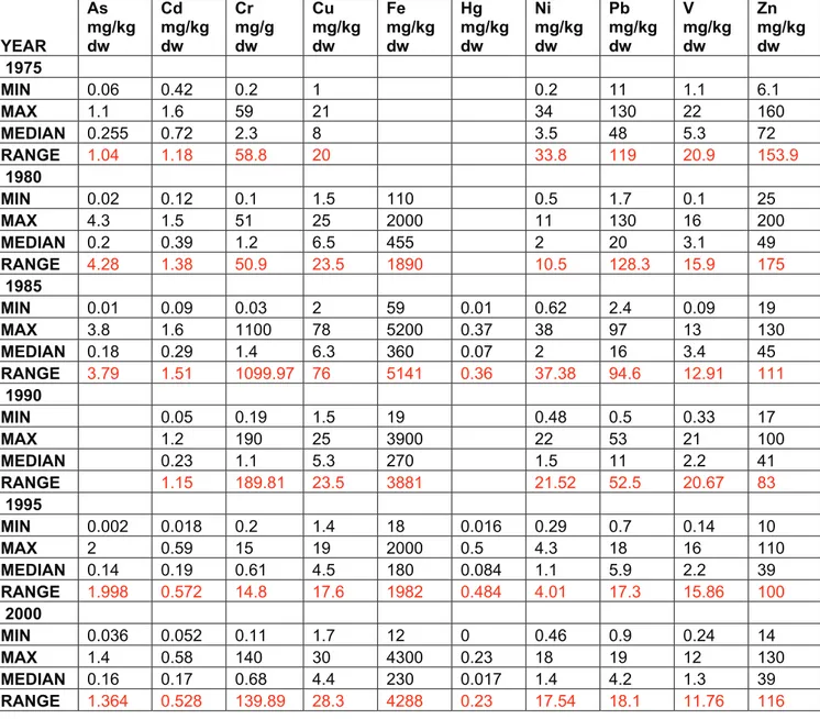
Table 3.2. Statistical summary of raw moss data (1975 – 2000).
YEAR As mg/kg dw Cd mg/kg dw Cr mg/g dw Cu mg/kg dw Fe mg/kg dw Hg mg/kg dw Ni mg/kg dw Pb mg/kg dw V mg/kg dw Zn mg/kg dw 1975 MIN 0.06 0.42 0.2 1 0.2 11 1.1 6.1 MAX 1.1 1.6 59 21 34 130 22 160 MEDIAN 0.255 0.72 2.3 8 3.5 48 5.3 72 RANGE 1.04 1.18 58.8 20 33.8 119 20.9 153.9 1980 MIN 0.02 0.12 0.1 1.5 110 0.5 1.7 0.1 25 MAX 4.3 1.5 51 25 2000 11 130 16 200 MEDIAN 0.2 0.39 1.2 6.5 455 2 20 3.1 49 RANGE 4.28 1.38 50.9 23.5 1890 10.5 128.3 15.9 175 1985 MIN 0.01 0.09 0.03 2 59 0.01 0.62 2.4 0.09 19 MAX 3.8 1.6 1100 78 5200 0.37 38 97 13 130 MEDIAN 0.18 0.29 1.4 6.3 360 0.07 2 16 3.4 45 RANGE 3.79 1.51 1099.97 76 5141 0.36 37.38 94.6 12.91 111 1990 MIN 0.05 0.19 1.5 19 0.48 0.5 0.33 17 MAX 1.2 190 25 3900 22 53 21 100 MEDIAN 0.23 1.1 5.3 270 1.5 11 2.2 41 RANGE 1.15 189.81 23.5 3881 21.52 52.5 20.67 83 1995 MIN 0.002 0.018 0.2 1.4 18 0.016 0.29 0.7 0.14 10 MAX 2 0.59 15 19 2000 0.5 4.3 18 16 110 MEDIAN 0.14 0.19 0.61 4.5 180 0.084 1.1 5.9 2.2 39 RANGE 1.998 0.572 14.8 17.6 1982 0.484 4.01 17.3 15.86 100 2000 MIN 0.036 0.052 0.11 1.7 12 0 0.46 0.9 0.24 14 MAX 1.4 0.58 140 30 4300 0.23 18 19 12 130 MEDIAN 0.16 0.17 0.68 4.4 230 0.017 1.4 4.2 1.3 39 RANGE 1.364 0.528 139.89 28.3 4288 0.23 17.54 18.1 11.76 116
CHAPTER FOUR: METHODS 4.1 Exploratory Data Analysis
“Exploratory Data Analysis (EDA) is an approach/philosophy for data analysis that employs a variety of techniques (mostly graphical) to maximize insight into a data set, uncover underlying structure, extract important variables, detect outliers and anomalies, test underlying assumptions, develop parsimonious models, and determine optimal factor settings” (NIST/SEMATECH, 2006).
EDA relies on graphic outputs to present its results that reinforce its exploratory nature. With this powerful graphic capabilities, the structure of the dataset is revealed in a way that other statistical approaches cannot, this of course is achieved with the aid of the human natural pattern recognition abilities. Some of the graphical techniques used in EDA are box plots, scatter plots, histograms, bi-histogram plots, etc. Unlike other classical quantitative statistical approaches, EDA uses all the available data in the dataset and employs little or no statistical assumptions in treating the data.
Among the software with EDA capabilities, XmdvTool (multivariate data visualisation tool) was used for the thesis; this was primary because of the ease of acquiring and setting it up and also usage (Ward, 2006). XmdvTool is a public-domain software package for the interactive visual exploration of multivariate data sets. It is available on all major UNIX/LINUX/MAC and Window platforms. XmdvTool is developed based on OpenGL and Tcl/Tk. It supports four methods for displaying flat form data and hierarchically clustered data: scatter plots, star glyphs, parallel coordinate plots, dimensional stacking.
Graphic interaction tools such as brushing, zooming, panning, masking and reordering of dimensions are all supported. The colour themes and flexibility of the user to choose varied colours makes it very adaptable to the user’s needs. It has been successfully applied in different fields such as environmental monitoring, demographic studies, remote sensing etc.
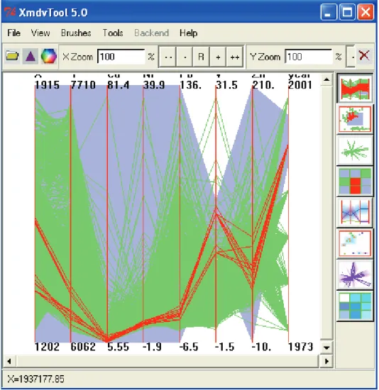
4.1.1 Parallel Coordinate Plot
Parallel coordinate plots are diagrams that display multi-dimensional data in a single plot or representation. The variables are represented by vertical lines with the maximum and minimum values at the top and bottom respectively. Observations at the same point are marked on the vertical lines (dimensions) and are linked together by a polyline. It has no limits as to dimensions or records, but mostly, displays with so many records are not easily comprehensible.
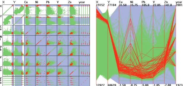
Example of a parallel coordinate plot is shown in Figure 4.1. In this figure, two clusters of vanadium on the 6th vertical axis from left are highlighted with red color. It is evident that these values form two clusters in space and they are all from the 1995 moss survey. Further information regarding the deposition values of the other elements at the same sample point can also be derived from the plot.
The parallel coordinate plots were applied during visual queries, data exploration and data cleaning.
Figure 4.1. Example of a parallel coordinate plot - moss survey 1975 – 2000.
4.1.2 Scatterplot
Scatter plot also referred to as scatter diagram or scattergram is a basic graphic tool that illustrates the relationship between two variables. The dots on the scatter plot represent the data points. They are used to study any possible relationship in variable data. Albeit it depicts a relationship between variables, it does not indicate any cause and effect relationship.
An example of scatterplot display of data is given in Figure 4.2. In XmdvTool the different displays are dynamically linked, meaning that highlighting samples in one window automatically affects all other displays. The scatterplot display shows that the two clusters in the 1995 vanadium deposition values (visible in Figure 4.1) seem to be located in the south western part of Sweden. The relationship of the vanadium clusters with the other elements can also be seen from the scatter plot.
Scatterplot visualization was applied during data exploration step to locate anomalies of different elements in space and time.
Figure. 4.2. Example of scatter plot - moss survey 1975 – 2000. 4.2 Geographic Information Systems
GIS can be defined in various ways based on different concepts and usage. It can be defined from the organisation – based, database and tool box – based aspects. From the tool box – based perspective, GIS could be defined as “ a powerful set of tools for collecting, storing, retrieving at will, transforming and displaying spatial data from the real world for a particular set of purposes” (Burrough & McDonnell, 2000).
Geographic information systems are made up of three components namely, computer hardware, software and organisational aspect comprising skilled personnel. Presently, GIS applications can be seen in almost every sphere of life primarily to store data, make maps and also for purposes of analysis and decision-making. These applications can be found in diverse disciplines such as agriculture, planning, environment, health etc.
One of the most popular desktop mapping software is ArcGIS desktop. It is a Windows based mapping software which has a bundle of applications grouped as ArcMap, ArcCatalog, ArcToolbox, Modelbuilder and ArcGlobe. These applications are used in database input and management, displaying maps, analysis, visualisations, geostatistics and many other tools available in the ArcGIS desktop (ESRI, 2006).
4.2.1 Visual Data Analysis
Like any survey or data collection exercise involving humans, there are uncertainties inherent in the data recorded. This could be caused by human factors, instrument malfunction and other factors. The presence of possible outliers was not ruled out of this project, therefore a very detailed visual analysis was done on the moss survey data to reveal possible outliers and to clean the data appropriately for further analysis. The data analysis was carried out in ArcGIS 9 and WINSTATS (WINSTATS, 2006). The moss data, saved as database files, were exported to ArcGIS 9. A shapefile was created for the point data and all the attributes cross-checked to ensure that they were all imported in the right format without any numerical approximations. The point data was then converted to layer files.
Considerations for removal of errors were done mutually exclusive of each other, meaning the levels of each sample were considered independently and outliers removed. Before any of the sample points were removed as outliers, an overview of the distribution of the data was studied carefully.
Box plot was the first method applied to the data. The results from the box plot are minimum value, maximum value, median, lower quartile, upper quartile and the suspected outliers shown as dots in the box. In some situation, the percentage of the data values between the lower quartile and median, the median and the upper quartile were shown. This was a very helpful insight into the data spread and data cleaning. The box plots were generated using the WINSTATS software.
25.00 200.00
25.00 49.00 84.00
42.00 59.00
Figure. 4.3. Example of a box plot (zinc, year 1980).
From Figure 4.3 the spread of the data is shown. From left to right, it shows the minimum value, lower quartile, median, upper quartile, maximum value and the highest outlier. The dots after the maximum value are all (possible) outliers. From the above Figure, we could also see that a number of high values tend to cluster in measurement space.
Histogram is tool that was used in the visual analysis of the data, leading to data cleaning. A histogram of each element in each of the surveys was plotted. From the histogram, the frequency of every value recorded was plotted and the spread was also noticed. Initially, the varying ranges of the elements made it difficult to uniformly display them in the histogram. For example, lead in 1975 had a minimum value of 11 mg/kg dw and maximum value of 130 mg/kg dw, however in 1980 it rather registered minimum 1.7 mg/kg dw and maximum 130 mg/kg dw. Chromium recorded a minimum of 0.03 mg/kg dw in 1985 and maximum 1100 mg/kg dw but in 1995 it recorded a minimum of 0.2 mg/kg dw and a maximum of 15 mg/kg dw. Using a standard range and class width for each element over the years solved this problem of
a uniform comparison between the different surveys. The range and class width were calculated as below:
Range (interval) = max – min (for all moss surveys), Class width = range/precision.
By this method, a comparative plot for each element over the survey years was displayed in the histogram. Possible clusters, extreme values and isolated values were then selected and highlighted in the map view. Suspected outliers selected in the histogram from geostatistical analyst were also highlighted in the map view of ArcMap. A check was done on the highlighted sample points to verify whether they are clusters or correlated with nearby values. In most cases, these suspected values were found to be unique with respect to their surrounding samples so they were treated as outliers. 25.00000 200.0 0 39 Freq Zn
Figure. 4.4. Example of a histogram (zinc, year 1980).
From Figure 4.4, the frequencies of the deposition values recorded are plotted with recorded deposition values. This shows how often certain concentration values were recorded and may help to decide whether these should be treated as outliers or not. The data spread in the box plots are similar to the spread in the histograms. The dots (outliers) in the box plots are relatively, spread similarly to the values in the histograms.
Though the decision of which recorded value are outliers or not remains very subjective, the combination of the two data display methods from ArcGIS and WINSTATS applied above provides a more decisive approach to visual data analysis leading to data cleaning.
4.2.2 Spatial Interpolation
“Interpolation is the procedure of predicting the value of attributes at unsampled sites from measurements made at point locations within the same area or region” (Burrough & McDonnell, 2000). It also used to convert point data into continuous surfaces so that the spatial patterns can be compared with other spatial entities. This is required mostly when the data at hand does not cover the entire area under study completely.
There are two main groupings of interpolation techniques: deterministic and geostatistical. Deterministic interpolation techniques create surfaces from measured points, based on either the extent of similarity (Inverse Distance Weighted) or the degree of smoothing (Radial Basis Functions). Geostatistical interpolation techniques (kriging) utilize the statistical properties of the measured points. Geostatistical techniques quantify the spatial autocorrelation among measured points and account for the spatial configuration of the sample points around the prediction location. Deterministic interpolation techniques can be divided into two groups, global and local. Global techniques calculate predictions using the entire dataset. Local techniques calculate predictions from the measured points within neighbourhoods, which are smaller spatial areas within the larger study area. Geostatistical Analyst provides the Global Polynomial as a global interpolation and the Inverse Distance Weighted, Local Polynomial, and Radial Basis Functions as local interpolators. Since the points in the moss dataset were sparsely populated all over Sweden, it was advisable to employ the global interpolation technique. Global Polynomial interpolation fits a smooth surface that is defined by a mathematical function (a polynomial) to the input sample points. The Global Polynomial surface changes gradually and captures coarse-scale pattern in the data (ESRI, 2006). Among other factors, the global interpolation technique is a quick and deterministic interpolator that is smooth and inexact. There are very few decisions to make when choosing model parameters and no assumptions required. A third order polynomial was chosen to create the surfaces, this was to reduce noise and at the same time create an interpolated surface similar to the real phenomena. Validation results from the global interpolation are automatically generated to show how similar the interpolated results are to the measured values.
The interpolated surfaces were constrained using an outline of Sweden, which served as the extent for all further raster analysis. The interpolated surfaces were converted to raster files in the ESRI GRID format with a resolution of one kilometre. The extent of the data coverage and the number of samples were the factors that influence this decision. This is because considering the transport or dynamics of the phenomena under study, a square kilometre cell size will suffice for the analysis.
4.3 Quantification of trends
The initial continuous surfaces created were at best to describe the individual elements in specific years. They were not sufficient to quantify the temporal changes and also for any comparative analysis. To arrive at the goal of this project, these surfaces were reclassified into ten levels of concentration. This method of classification adopted was only a relative scale and not absolute. To achieve these reclassifications, the minimum and maximum values for an element during all moss
surveys were used to calculate the total range of concentrations, which was then rescaled into 10 classes. The maximum value was assigned 100 % and the rest were divided into equal class intervals as shown in Table 4.1.
Table 4.1. Relative scale to quantify pollution loads (mg/kg dw). ELEMENT MIN MAX 0-10%
10-20% 20-30% 30-40% 40-50% 50-60% 60-70% 70-80% 80-90% 90-100% Cu 1 13 1,3 2,6 3,9 5,2 6,5 7,8 9,1 10,4 11,7 13 Ni 0,2 6,5 0,65 1,3 1,95 2,6 3,25 3,9 4,55 5,2 5,85 6,5 Pb 0,5 95 9,5 19 28,5 38 47,5 57 66,5 76 85,5 95 V 0,1 21 2,1 4,2 6,3 8,4 10,5 12,6 14,7 16,8 18,9 21 Zn 10 110 11 22 33 44 55 66 77 88 99 110
For every element in the moss survey, the values were reclassified into these ten classes. The resulting reclassified raster files were assigned the same cell size as the spatial interpolation to ensure uniformity and also comparable results. From the attribute table of the reclassified raster surfaces, the cell count was extracted for each class. From this, the amount of cells each of the five levels of concentration was made up of in any element was tabulated. The benefit of this approach is to put the variations in the interpolated surfaces into very distinct classes for easy identification of trends and also to quantify the trends. In some situation, there were few no data areas, but their effect on the outcome was considered insignificant since their numbers were very few compared to the total cell count.
CHAPTER FIVE: RESULTS AND DISCUSSION 5.1 Data Cleaning
The data cleaning process yielded noticeable change in some qualities such as number of samples, range, minimum and maximum values and median. It was now possible to obtain better histograms of each element. Due to inconsistencies in some sampled elements over the years, not all the initial elements were considered for the final analysis. For instance, arsenic (As), iron (Fe) and mercury (Hg) were not sampled in some of the surveys. Cadmium (Cd) and chromium (Cr) had insufficient sampled point for some surveys. After careful considerations, copper (Cu), nickel (Ni), lead (Ni), vanadium (V) and zinc (Zn) were selected for the final analysis due to their consistency of reasonable samples for all the surveys.
The data cleaning was considered successful because a more reliable dataset was obtained without so much loss of initial data. In some elements, very few data points were lost while there was a remarkable improvement in the statistical qualities of the dataset.
Comparing Tables 3.1 and 5.1, it is obvious that there has not been any significant change in the number of samples, but a further comparison of Tables 3.2 and 5.2 will reveal a significant improvement in the statistical qualities of the moss data. While the ranges of concentration show significant decrease, the median values present only a slight decrease due to removal of the highest concentrations. That can be taken as an
indication for very skewed original distributions, caused by a number of single very high-valued outliers.
Table 5.1. Summary of sample count of clean moss data (1975 – 2000).
YEAR Cu Ni Pb V Zn 1975 273 266 273 268 263 1980 787 790 806 795 790 1985 897 899 903 888 905 1990 826 821 826 819 819 1995 980 981 948 788 983 2000 571 571 575 569 573
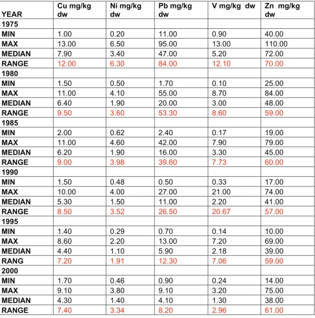
Table 5.2. Statistical summary of clean moss data (1975 – 2000).
YEAR Cu mg/kg dw Ni mg/kg dw Pb mg/kg dw V mg/kg dw Zn mg/kg dw 1975 MIN 1.00 0.20 11.00 0.90 40.00 MAX 13.00 6.50 95.00 13.00 110.00 MEDIAN 7.90 3.40 47.00 5.20 72.00 RANGE 12.00 6.30 84.00 12.10 70.00 1980 MIN 1.50 0.50 1.70 0.10 25.00 MAX 11.00 4.10 55.00 8.70 84.00 MEDIAN 6.40 1.90 20.00 3.00 48.00 RANGE 9.50 3.60 53.30 8.60 59.00 1985 MIN 2.00 0.62 2.40 0.17 19.00 MAX 11.00 4.60 42.00 7.90 79.00 MEDIAN 6.20 1.90 16.00 3.30 45.00 RANGE 9.00 3.98 39.60 7.73 60.00 1990 MIN 1.50 0.48 0.50 0.33 17.00 MAX 10.00 4.00 27.00 21.00 74.00 MEDIAN 5.30 1.50 11.00 2.20 41.00 RANGE 8.50 3.52 26.50 20.67 57.00 1995 MIN 1.40 0.29 0.70 0.14 10.00 MAX 8.60 2.20 13.00 7.20 69.00 MEDIAN 4.40 1.10 5.90 2.18 39.00 RANG 7.20 1.91 12.30 7.06 59.00 2000 MIN 1.70 0.46 0.90 0.24 14.00 MAX 9.10 3.80 9.10 3.20 75.00 MEDIAN 4.30 1.40 4.10 1.30 38.00 RANGE 7.40 3.34 8.20 2.96 61.00
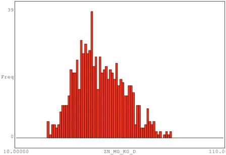
The change in histogram shape can be observed comparing Figures 5.1 and 5.2. With the removal of the outliers, the form of the histograms is not skewed to one side due to the presence of a few outliers. They are more legible in the plot window.
The results described above show that using graphics or visual analysis in outlier detection for data cleaning is a very useful approach to reduce the loss of data and at the same time maintaining the primary characteristics of the data. This also helps a lot in minimising our biases in data cleaning which cannot entirely be free from subjectivity. 10.00000 110.00 39 Freq 0 ZN_MG_KG_D
Figure 5.1. Histogram of clean zinc data (2000). 5.2 Data Exploration
The use of GIS and visualisation tools unravelled some trends and intriguing information about the moss surveys over the years. To begin with, the EDA gave us an insight into how this multivariate data was related to each other and the distribution of the outliers. The comparison brought to fore the different levels of outliers in different years of the survey. In some years, the outlier concentration value would easily pass for an acceptable concentration value in other years. This initially prompted the idea to clean the data element-by-element basis for each survey. Some observations from the data exploration are:
• Contrary to the notion that the first moss survey in 1975 recorded generally high values of elements due to high pollution loads, there were however instances where very low deposition values. These low or censored values under the detection limit can be located by EDA to visualize the levels of other elements recorded at the same sample. An example is given in Fig. 5.2. One can see that the lowest two concentrations of Cu in 1975 are not higher than the lowest concentrations of the same element in other surveys. Moreover, these two samples contain relatively high concentrations of other elements (seen from the parallel coordinate plot). The exact concentrations can be
plotted, to find out whether the levels of Cu were under the lowest detection limit in those samples.
Figure 5.2. Scatter plot (left) and Parallel coordinate plot (right) of moss data.
Figure 5.3. Scatterplot (left) and parallel coordinate plot (right) showing the position of trend of north eastern tip of Sweden.
Figure 5.3 presents results from a query defined in coordinate space. All samples belonging to all surveys within a rectangular area in north-eastern Sweden were selected in scatterplot display. The correlations between elements in the highlighted samples can be seen in the scatterplot display, and the relative concentration ranges are visible in parallel coordinate plot. One can see that there is a relatively good correlation between the concentrations of following elements: Cu-Pb, Cu-V, Pb-V. Ni presents a considerable anomaly that does not involve any other metals. The rightmost column in the scatterplot display indicates that the anomaly can be related to years 1985, 1990 and 2000.
General trends instead of details can also be explored during interactive visualization and querying. In Figure 5.4 the northern Sweden was selected, highlighting about two
thousand samples. The shape of scatterplots suggests that correlations between elements differ for northern and southern parts of Sweden. The parallel coordinates display visualizes how large part of the total concentrations ranges can be related to the north of Sweden. Interestingly, copper and nickel recorded relatively high deposition rates as compared to the other elements. However, there was no sampling of the north in the 1975 survey.
Figure 5.4. Parallel coordinate plot (left) and scatterplot (right) showing pollution load of Northern Sweden (1975 – 2000).
From Figure 5.5, we know that southern Sweden recorded high pollution loads as compared to northern Sweden. On the contrary, nickel and copper recorded relatively low deposition ranges. Southern Sweden is also densely sampled as compared to northern Sweden and has been covered in all the moss surveys.
Figure 5.5. Parallel coordinate plot (left) and scatterplot (right) showing pollution load of Southern Sweden (1975 – 2000).
It is worth mentioning that, the trends and relationships to unravel using EDA are limitless and the users and curiosity and imagination can lead to very interesting and
inconspicuous details. It is also important to toggle between the parallel coordinate plot and the scattergram to get a detailed insight into the data.
5.3 Spatial Interpolation
From the results of the spatial interpolation, it was possible to observe a nationwide deposition rate over the years. Some examples of the interpolated maps as shown above in Figures 4.7 and 4.8 clearly show the continuous spatial trends in deposition of the element under study. To ensure that the interpolated surfaces are near to reality as possible, a cross validation table from the interpolation process was saved. From the table, it was evident that the magnitude of errors was varying. The error is the difference between the measured value and the predicted value. Table 4.1 presents the tabulated mean and median values of the spatial interpolation. For the purpose of comparison, the measured and predicted values of the spatial interpolation as well as their associated errors are shown in Table N1 and N2 of appendix N.
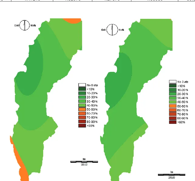
From Figure 5.6 one can easily be misled into thinking that both interpolated surfaces are the same or very similar, except the difference in the eastern and south-western deposition values. This however is not the real situation since from the reclassified maps of nickel and copper shown below (Figure 5.7), there are distinct variations in the deposition values revealed through the quantification method adopted.
Table 5.3. Summary of median of deposition values from spatial interpolation results. YEAR Cu(mg/kg dw) Ni(mg/kg dw) Pb (mg/kg dw) V(mg/kg dw) Zn(mg/kg dw)
1975 7.90000 3.40000 47.00000 5.20000 70.00000 1980 6.30000 1.90000 20.00000 3.00000 48.00000 1985 6.10000 1.90000 16.00000 3.30000 44.00000 1990 5.30000 1.50000 11.00000 2.20000 41.00000 1995 4.40000 1.10000 5.90000 2.18000 39.00000 2000 4.30000 1.40000 4.10000 1.30000 38.00000
Table 5.4. Summary of mean deposition values from spatial interpolation results. YEAR COPPER(mg/kg dw) NICKEL(mg/kg dw) LEAD (mg/kg dw) VANADIUM(mg/kg dw) ZINC(mg/kg dw) 1975 8.08400 3.46800 49.50700 5.62700 70.59900 1980 6.35100 2.00090 21.92100 3.29300 41.31960 1985 6.19300 2.03190 16.66600 3.34020 44.19740 1990 5.40050 1.59100 11.31800 2.37050 41.46030 1995 4.58350 1.11140 6.01570 2.21280 39.59520 2000 4.47210 1.52070 4.27570 1.35980 39.38090
Figure 5.7. Maps of copper and nickel deposition loads (2000).
To assess the reliability of the spatial interpolation was crucial in this project, though no interpolation technique is perfect, a conscious effort was made to create an interpolated surface as close as possible to the real surface. This was ensured by automatically creating a cross validation results then analysing the measured and predicted values of each interpolated surface. In the analysis, we tried to look at the smoothing effects of the interpolation method, and instances where the new values created or lost were higher or lower than the measured value. A scatter plot of the cross validation results presented the cross-validation results in detail. For lack of space, only few distinct cases are discussed below.
0,00 5,00 10,00 15,00 20,00 25,00 30,00 35,00 40,00 45,00 0,00 5,00 10,00 15,00 20,00 25,00 30,00 35,00 40,00 45,00 MEASURED PREDICTED
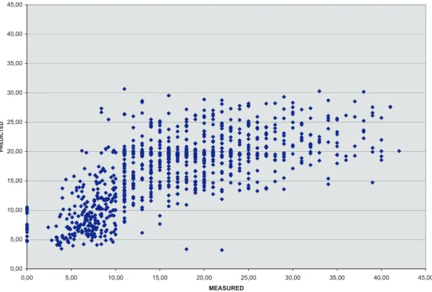
Figure 5.8. Scatter plot of cross validation results for lead 1985.
An interpolation that honours all known values would show a scatterplot where all values (points) area aligned along the diagonal from lower left to upper right corner. Instead, a point cloud is formed, indicating that the quality of prediction varies locally, creating a range of predicted concentrations for the same measured concentrations. When the predicted values are considerably lower or higher that the measured ones, the direction of the point cloud fails to follow the diagonal of the graph. This happens most often for the concentrations that are the lowest or highest along the measured range.
From Figure 5.8 above, we can see that there was smoothing on the measured values reaching 20-25 mg/kg. Comparatively the lowest measured values got up to 5-10 mg/kg higher prediction values. The point cloud has a curve towards horizontal direction from about 15 mg/kg. Another conclusion is that there is a substantial local variation in the concentration of Pb in 1985, which can be confirmed by Fig. K3. in appendix K.
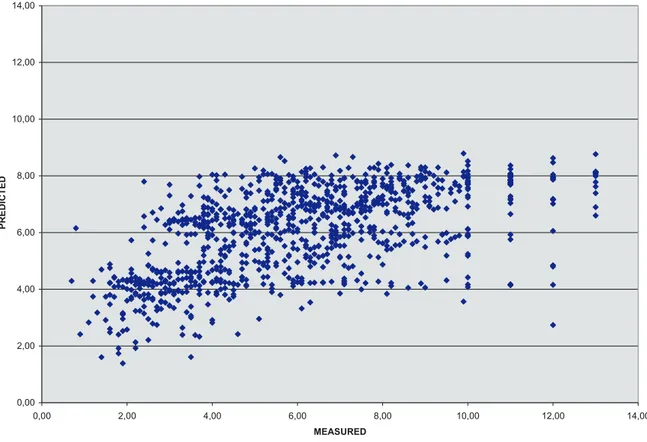
Comparing the summary statistics of Table N2 in appendix N, the measured median value of lead in 1985 was 16.00 mg/kg dw but the predicted median value is 18.20190 mg/kg dw with a corresponding median error of 0.76830. The mean values were 16.66660 mg/kg dw for measured and 16.66670 mg/kg dw for prediction with an error of 0.00140. These numerical results suggest that, in general, the surface fitting can be considered good. However, one can conclude from the scatterplot illustration that significant under- or overestimation of element concentrations can take place locally. The cross validation scatterplot for interpolated surface of lead in 1995 (Fig. 5.9) is one of the most detailed and interesting. One of the reasons can be the relatively small range of concentrations, revealing details in the distribution of concentrations. Obviously the same element has different distribution of lows and highs from year to year, resulting in different degree of surface fitting (see also Fig. 5.8). The scatter plot in Figure 5.8 presents similar shape of point cloud while the smaller concentration range means that the under- and overestimation by interpolation is less, up to 6 mg/kg. The scatterplot also suggest clustering of concentrations between 2 and 4 mg/kg. This probably points to presence of strong regional spatial patterns in the distribution of concentrations.
From the summary statistics in Table N1 and N2 of appendix N, the measured median value of 5.9 mg/kg dw and the predicted median was 6.2 mg/kg dw with a median error 0.24200 mg/kg dw while the mean measured was 6.01570 mg/kg dw and the predicted was 6.01690 mg/kg dw with an error of 0.00130.
0,00 2,00 4,00 6,00 8,00 10,00 12,00 14,00 0,00 2,00 4,00 6,00 8,00 10,00 12,00 14,00 MEASURED PRE D IC T E D
Figure 5.9. Scatter plot of cross validation results for lead 1995.
From Tables N1 and N2 in appendix N, vanadium recorded a median value of 2.2000 mg/kg dw and a median predicted value of 2.55960 mg/kg dw with an error of 0.19800. The mean recorded value was 2.37050 mg/kg dw, predicted mean was 2.37020 mg/kg dw with an error of 0.00028. The scatter plot (Fig. 5.10) is a good illustration for the influence of single extreme values for the range of concentrations and the appearance of a scatterplot. The original range of 0-21 mg/kg decreased to 1-4 mg/kg. Due to single extreme outliers the details in the distribution of values in the point cloud is no longer visible. This is one of the reasons for undertaking careful data cleaning before interpolation. Because the surrounding samples normally have much lower concentrations the single high concentration will most often disappear during the interpolation.
The scatter plots from the cross validation points were useful in revealing some prediction values that otherwise are not possible from simple statistical summaries. The general observations from the cross validation results point to the loss of local high values and overestimation of concentrations at the low end of the measured axis. That is, most measured low values are predicted slightly higher whereas measured high values are predicted lower. This depends on the spatial distribution of the pollution loads, and the smoothing degree of the interpolator. As a global interpolator was used these effects can be considered normal.
One interesting detail that was revealed by cross-validation scatterplots was the fact that all measured concentrations less than 10 mg/kg seem to have a precision of 0.01 while concentrations over 10 mg/kg have a precision of 0.1 mg/kg.
0,00 5,00 10,00 15,00 20,00 25,00 0,00 5,00 10,00 15,00 20,00 25,00 MEASURED PR ED IC TE D
5.4 Spatial Trends
The results of the interpolation differ from the results of IVL due to the different methods employed in the interpolation. The general spatial trends were however similar. The interpolation method applied produced very smooth surfaces; it was therefore necessary to use at least 10 classes, to be able to visualize variation in concentration. Considering the relative scale of concentrations and large differences between the surveys, it could be beneficial to consider even 15 or 20 classes. The relative scale may however not be the best for revealing spatial trends for the surveys reporting low deposition values.
Comparing the respective maps in Appendices A and H show that the polynomial interpolation used was not suitable for predicting a surface that represents the variation in metal deposition. The spatial patterns that are limited in space are overlooked while interpolation introduces unwanted side-effects in the form of artificial patterns. These can often be seen in interpolated survey data from 1975, due to the facts that measurements from only southern part of Sweden were available, and that the pollution loads were generally high. Thus the quality of prediction varies substantially for the same element in different surveys.
To sum up, the interpolated maps did not reveal any new information about the spatial trends in element concentrations.
5.5 Temporal Trends
The temporal trends are presented in visual results (Appendix A) and using numerical approach. While the relative scale used to reclassify interpolated surfaces was not relevant for visualizing spatial trends, it is well suited for revealing the temporal changes in deposition loads over the years. Interpolation results for each element and year showed (chapter 5.4) that the median concentrations in original and interpolated datasets did not differ much. However, the interpolation technique was not very suitable and further conclusions about the actual magnitude of changes cannot therefore be made. The importance of data cleaning to the results and interpretation should not be underestimated.
A cursory look at the numerical results shows that the zinc has the highest median deposition value for all the year (1975 – 2000). The rest follows the order of lead, copper, vanadium and lastly nickel. Generally there has been a rapid decrease in concentrations, which strongly indicates a remarkable improvement in the quality of air within the study area.
Table 5.5. Year-to-year rate of change of deposition (based on median values).
ELEMENT 1975 - 1980 1980 - 1985 1985 - 1990 1990 - 1995 1995 - 2000 1975 - 2000 COPPER -20.25% -3.17% -13.11% -16.98% -2.27% -45.57% NICKEL -44.12% 0.00% -21.05% -26.67% 27.27% -58.82% LEAD -57.45% -20.00% -31.25% -46.36% -30.51% -91.28% VANADIUM -42.31% 10.00% -33.33% -0.91% -40.37% -75.00% ZINC -31.43% -8.33% -6.82% -4.88% -2.56% -41.71% 25
From Table 5.5, it is very evident that, there have been decreasing rates of change in the various elements over the year. But we should also not disregard to slight increasing changes in the concentration values. This can be seen in reasonable percentages in nickel (27.27%, 1995 – 2000). Vanadium also registered some increased rate changes 1980 – 1985.
The overall rate of change in the mean deposition values shows lead leading followed by vanadium, nickel, copper and lastly zinc. This shows that in spite of the remarkable improvement in the air quality, zinc still posses a problem in terms of the level of concentration recorded in the survey.
The results in Table 5.5 can be summarised in Figure 5.11. This gives a graphical interpretation to the rate of change of pollution loads for each element from one moss survey to the next.
Figure 5.11 shows a decrease in the deposition loads for all elements from 1975 to 1980, however, vanadium increased about 10% from 1980 to 1985. The subsequent years showed a general decrease in deposition loads, though vanadium showed just a slight decrease. Nickel, uncharacteristically, showed a 27% increase in deposition loads from 1995 – 2000. This change was unusual since there was general trend of deposition load reduction.
-60,00% -50,00% -40,00% -30,00% -20,00% -10,00% 0,00% 10,00% 20,00% 30,00% RATE OF CHANGE (%) 1975 - 1980 1980 - 1985 1985 - 1990 1990 - 1995 1995 - 2000 TIME (YRS) COPPER NICKEL LEAD VANADIUM ZINC
Figure 5.11. A graph of rate of change of deposition (based on median values).
These general temporal trends discussed above, were deemed inadequate for a detailed quantification of temporal changes. Therefore a local approach was taken to study the regional temporal trends.
The results showed varied trends in the south, middle and northern portions of Sweden. This is tabulated below.
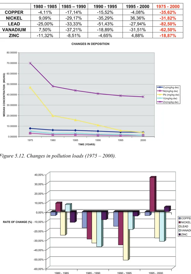
Table 5.6. Year-to-year rate of deposition for northern Sweden. 1980 - 1985 1985 – 1990 1990 - 1995 1995 - 2000 1975 - 2000 COPPER -4,11% -17,14% -15,52% -4,08% -35,62% NICKEL 9,09% -29,17% -35,29% 36,36% -31,82% LEAD -25,00% -33,33% -51,43% -27,94% -82,50% VANADIUM 7,50% -37,21% -18,89% -31,51% -62,50% ZINC -11,32% -8,51% -4,65% 4,88% -18,87% CHANGES IN DEPOSITION 0.00000 10.00000 20.00000 30.00000 40.00000 50.00000 60.00000 70.00000 80.00000 1975 1980 1985 1990 1995 2000 TIME (YEARS) MED IAN CO N C E N TRAT IO N (MG /KG) Cu(mg/kg dw) Ni(mg/kg dw) Pb (mg/kg dw) V(mg/kg dw) Zn(mg/kg dw)
Figure 5.12. Changes in pollution loads (1975 – 2000).
-60,00% -50,00% -40,00% -30,00% -20,00% -10,00% 0,00% 10,00% 20,00% 30,00% 40,00% RATE OF CHANGE (%) 1980 - 1985 1985 - 1990 1990 - 1995 1995 - 2000 TIME (YRS) COPPER NICKEL LEAD VANADIUM ZINC
Figure 5.13. Bar chart of rate of deposition for northern Sweden.
From the bar chart above (Figure 5.12), northern Sweden recorded decreasing deposition rates for copper (-4.11%), lead (-25%) and zinc (-11.3%) between 1980 and 1985 whiles nickel and vanadium increased by 9.09% and 7.5% respectively. Between 1985 and 1995, all the five elements recorded a decrease in deposition loads from the previous years. Nickel rapidly increased by 36.36% between 1995 and 2000 whiles zinc also showed a modest increase in the rate of deposition by 4.88%.
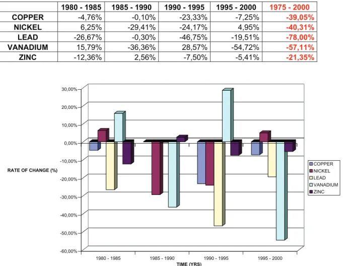
Table 5.7. Year-to-year rate of deposition for mid Sweden.
1980 - 1985 1985 - 1990 1990 - 1995 1995 - 2000 1975 - 2000 COPPER -4,76% -0,10% -23,33% -7,25% -39,05% NICKEL 6,25% -29,41% -24,17% 4,95% -40,31% LEAD -26,67% -0,30% -46,75% -19,51% -78,00% VANADIUM 15,79% -36,36% 28,57% -54,72% -57,11% ZINC -12,36% 2,56% -7,50% -5,41% -21,35% -60,00% -50,00% -40,00% -30,00% -20,00% -10,00% 0,00% 10,00% 20,00% 30,00% RATE OF CHANGE (%) 1980 - 1985 1985 - 1990 1990 - 1995 1995 - 2000 TIME (YRS) COPPER NICKEL LEAD VANADIUM ZINC
Figure 5.14. Bar chart of rate of deposition of mid Sweden.
The middle portion of Sweden (from Figure 5.13 and Table 5.5) exhibits the same pattern of rate of change as the global temporal trend in the whole Sweden. Lead has the highest rate of change of deposition with zinc having the least. All the years recorded some increase and decrease in rates of deposition. Only zinc recorded a modest increase between 1985 and 1990 whiles vanadium increased about 28% between 1990 and 1995. Nickel also showed a modest increase between 1995 and 2000.
It should be mentioned that, the 1974 moss survey was carried out only in southern Sweden hence the regional trends for northern and mid Sweden were all from 1980 to 2000.
Table 5.8. Year-to-year rate of deposition for southern Sweden. 1975 - 1980 1980 - 1985 1985 - 1990 1990 - 1995 1995 - 2000 1975 - 2000 COPPER -0,38% 2,04% -6,00% -23,40% 8,33% -50,63% NICKEL -0,53% 0,00% -12,50% -28,57% 0,20% -64,71% LEAD -74,47% -34,17% -30,38% -36,36% -37,14% -95,32% VANADIUM -60,58% -26,83% 0,00% 6,67% -45,63% -83,27% ZINC -37,14% -13,64% -7,89% -5,71% -12,12% -58,57% -80,00% -70,00% -60,00% -50,00% -40,00% -30,00% -20,00% -10,00% 0,00% 10,00% RATE OF CHANGE (%) 1975 - 1980 1980 - 1985 1985 - 1990 1990 - 1995 1995 - 2000 TIME (YEARS) COPPER NICKEL LEAD VANADIUM ZINC
Figure 5.15. Bar chart of rate of deposition for southern Sweden.
Reference to Figure 5.14 and Table 5.6, Southern Sweden recorded the highest reduction in pollution loads from 1975 to 1980, between these years, lead recorded the highest decrease of 74.47%, followed by vanadium (60%) then zinc (37.14%). Copper and nickel however recorded very moderate decrease in pollution loads. Only copper recorded an increase in rate of pollution from 1980 to 1985 and 1995 and 2000.
From the regional rate of deposition, we could see some changes that were not possible in the global rate of change in Figure 5.10. From the national perspective, as shown in Figure 5.10, only nickel and vanadium showed an increase in the rate of change by 27.27% and 10% between 1995 and 2000 and 1980 and 1985 respectively. Contrary to the aforementioned, zinc, also showed some increase in pollution loads in northern Sweden by 4.48% between 1995 and 2000. In the middle part of Sweden, zinc again recorded some modest increase in pollution loads by 2.56% between 1985 and 1990, actually it was the only element that recorded a rise in those years. Southern Sweden recorded a rise in copper pollution loads by 2.04% from 1980 to 1985 and 8.33% from 1995 to 2000. Nickel and vanadium also recorded some increases in southern Sweden.
One can infer from Figures 5.12 to 5.13 and Tables 5.3 to 5.5 that, the recorded increase in the pollution loads of some elements correspondingly cause their low rate of change in deposition. This is seen in copper deposition rates for southern Sweden.
CHAPTER SIX: CONCLUSIONS AND RECOMMENDATIONS 6.1 Conclusions
From the summaries above, one can have a better insight into the temporal trends of the deposition rates as well as the changes in the trends over the geographic space. This has not been the emphasis in most previous studies. Generally, there has been a remarkable reduction in concentration levels of the element over time. It can then be said that the quality of air has improved considerably over the years.
Comparatively, southern Sweden has always recorded higher levels of concentration than the rest of the country. There is a nationwide decrease in the levels as one move towards northern Sweden. From this project, the seeming incomprehensible moss survey data has been cleaned, visualised and analysed in a very simplistic way using exploratory data analysis and GIS methods. It has succeeded in showing the possibility of shifting the emphasis of the analysis of the survey results from purely numerical classical statistical methods to more visual EDA and GIS analysis. This will greatly enhance the understanding of the data by more people, not just specialists. With more people understanding the changes in the environment in very simple way, the chances of a greater collaborative effort in combating environmental degradation can be assured.
Below is a summary of the conclusions drawn from this project
From the statistical summaries and plots, one can have a better insight into the regional temporal trends of the deposition as well as the changes in the trends over geographic space.
Global polynomial interpolation did result in serious under- and overestimation of predicted concentrations. Some of the explanations could be irregular and varying sampling density, both spatial and temporal, combined with highly varying deposition loads.
Multi-element visual data analysis proved to be helpful for data cleaning and detecting multi-element spatial patterns.
Scatter plot presentation of cross-validation results is a useful tool for visualizing different precision in original data as well as quantifying smoothing effect of interpolation technique.
The advantages with a relative concentration scale for presenting temporal data may result in better visualization of regional trends and temporal variations.
The seemingly incomprehensible moss survey data has been cleaned, visualised and analysed in a very simplistic way using exploratory data analysis and GIS methods.
6.2 Recommendations
• There is a need to consider the importance of GIS and visualisation techniques in the design of such survey to enhance the analysis of the results.
• More attention should be given to the spatial aspects involved in such surveys at the planning and data collection stages. This will greatly improve data display and analysis in the end.
• For future research, there could be an investigation into the transport and dynamics of the elements being measured to know where they are coming from and the possible changes they may have gone through along the way. This should not just be a purely chemical or environmental exercise, but should incorporate spatial analysis and GIS.
• The possible sources, causes and reasons for the changes in deposition and the relationship with geographical space could be another interesting collaborative research in future.
• Finally, there should be a concerted effort to make the results of such surveys very understandable in very simple ways to the layman.