CMC. doi:10.32604/cmc.2020.08885 www.techscience.com/journal/cmc
Stochastic Numerical Analysis for Impact of Heavy Alcohol
Consumption on Transmission Dynamics of Gonorrhoea Epidemic
Kamaleldin Abodayeh1, Ali Raza2, *, Muhammad Shoaib Arif2, Muhammad Rafiq3,
Mairaj Bibi4 and Muhammad Mohsin5
Abstract: This paper aims to perform a comparison of deterministic and stochastic models. The stochastic modelling is a more realistic way to study the dynamics of gonorrhoea infection as compared to its corresponding deterministic model. Also, the deterministic solution is itself mean of the stochastic solution of the model. For numerical analysis, first, we developed some explicit stochastic methods, but unfortunately, they do not remain consistent in certain situations. Then we proposed an implicitly driven explicit method for stochastic heavy alcohol epidemic model. The proposed method is independent of the choice of parameters and behaves well in all scenarios. So, some theorems and simulations are presented in support of the article.
Keywords: Heavy alcohol model, stochastic techniques, stability analysis. 1 Literature survey
Addiction and dependence on alcohol is an illness which involves inclination for drinking alcohol without stopping and without giving any heed to its negative repercussions on the health, relationships and social standing [Room, Babor and Rehm (2005)]. Like all other drug afflictions, dependence on the drug is deemed to be curable. According to the WHO’s study, approximately 140 million people are drug addicts in the world, and they are the victims of many alcohol-related issues for example illness, getting fired from the job and several other similar problems [Saunders, Aasland, Amundsen et al. (1993)]. Deplorably, biological causing of addiction to alcohol is not yet known. Nonetheless, age, sex, depression, social milieu, and mental state are a few factors which may contrive in exposing a person to alcoholism [Kozlowski and Agarwal (2000); Chen, Storr and Anthony (2009)]. Consumption of alcohol for a long period may cause hazardous changes in the brain, for example, intolerance and dependence on others. Delicate
1 Department of Mathematics and General Sciences, Prince Sultan University, Riyadh, Saudi Arabia.
2 Stochatic Analysis & Optimization Research Group, Department of Mathematics, Air University, PAF
Complex E-9, Islamabad, 44000, Pakistan.
3 Faculty of Engineering University of Central Punjab, Lahore, Pakistan.
4 Department of Mathematics, Comsats University, Chak Shahzad Campus park road, Islamabad, Pakistan. 5 Department of Mathematics, Uppsala University, Uppsala, Sweden.
changes are responsible for making it difficult for alcoholics to leave drinking, and quitting alcohol also causes some changes. There is hardly any part of the body which is not badly affected by the consumption of alcohol. It causes several diseases may damage destruction of the liver, pancreatitis, reproductive system and also of the nervous system [Walter, Gutierrez, Ramskogler et al. (2003); Benedict (2007); Testino (2008); Blum, Nielsen and Riggs (1998)]. There are several ways to get rid of alcohol which includes self-restraint, family support, therapy and medicines, but approximately seventy to eighty per cent addicts recover after treatment. Gonorrhoea is a disease which passes through sex. It bents on infecting warm, moist areas of the body such as parts of urine, eyes, throat, vagina, anus and female reproductive tract (the fallopian tubes, cervix, and uterus). The correct history of gonorrhoea cannot be traced. Historical records of the disease dating 1161 when the English parliament promulgated a law to guarantee that the transmission of the infection is checked and exterminated. In 1879 Neisser discovered the gonococcus or Neisseria gonorrhoeae and very soon it proved to be the very cause of gonorrhoea. He proved its existence consistently in patients with symptoms. Diseases which may be transmitted through sex except HIV are a cause of a large number of illness throughout the world, adults aged between 15 to 49 are the greatest victims of the sexually transmitted illnesses throughout the world; approximately 340 million new cases of STI’s appear among these adults every year globally presented in Agusto et al. [Agusto and Okosun (2010)]. Collectively, HIV and sexually transmitted infections (STIs) are a cause of damage to health on a large scale throughout the world. Gonorrhoea transmits from people to people through different forms of unsafe sexual intercourse, e.g., oral, anal, and vaginal sex. Those having multiple sexual relationships or don’t use a condom are prone to be the victim of this disease. Newly born children may also be the victims of this disease due to eye infection. Usually, infected women show no signs of illness, but all infected men and women carry disease even if signs of illness disappear. Gonorrhoea can become the cause of epididymitis, a very excruciating state in which testicles are badly infected and may lead to infertility if proper treatment is no taken. Those who contract the infection in the throat due to oral sex feel pain in the throat. The most protective way is not to have sex at all or to restrict sexual relationship with only one partner and also to use a condom for sex. Gonorrhoea commonly shows its symptoms within fourteen days of infection. Mercury was used to curing gonorrhoea in the past. Records from an English warship “Mary Rose” reveal that different kinds of instruments were used to inject Mercury in the human body through urinary parts. Silver nitrate was used to cure gonorrhoea in the nineteen centuries. The first vaccine was prepared in the 1890s from killed gonococci taken from Neisser’s laboratory. This vaccine was introduced in 1909. Other drugs to cure this disease were in use until the 1940s when antibiotics especially Penicillin, came into use. A bird’s eye view of previous studies on the subject gives us a reference to this paper. Different abstract has been conducted on alcohol spread factors which cause numerous complications. Gonorrhoea and other sexually transmitted infections models have presented in 1996 by Chavez et al. [Chavez, Huang and Li (1996)]. The researchers endorsed an opinion in behaviorally and genetically analogous population’s coexistence is not feasible but under very rare conditions. No study has regarded the effects of alcohol on the spread of gonorrhoea. Hence, in this context, that our observation reveals the relatedness and stimulation, by
developing a mathematical model to inquire the effects of massive drinking of alcohol on the spread dynamics of gonorrhoea disease in the society. The main purpose of the study is to predict developments in the events of gonorrhoea disease and also to the relationship between heavy consumption of alcohol in the community.
The main question of this article is to restore the dynamical properties of the model by developed stochastic technique [Mickens (1994, 2005, 2005)]? So, we shall construct the implicitly driven explicit technique for the given model under the rules presented by Mickens.
This article based on the following sections:
In the second section, we will describe the simple deterministic heavy alcohol model. We presented the stochastic heavy alcohol model and their symmetries in the third section. In the fourth section, we have presented the stochastic numerical techniques for model and their stability analysis. In the fifth section, we have presented the results discussion and coming directions.
2 Deterministic heavy alcohol model
In this section, we consider the heavy alcohol model presented in Bonyah et al. [Bonyah, Khan, Okosun et al. (2019)].
The description of variables at any time t is as follows: Sd(t) (denotes the susceptible
heavy alcohol drinkers in time t), Id(t) (denotes the heavy alcohol drinkers who are
infected by gonorrhoea in time t), R(t) (denotes the individuals recovered from gonorrhoea in time t). The flow of heavy alcohol epidemic model as shown in Fig. 1.
The model parameters are described as Λ (denotes the human recruitment), µ (denotes the natural and due to infection mortality rate), λ (denotes the rate of heavy drinkers), ν (denotes the waning rate), b (denotes the proportion, non-heavy alcohol drinkers), 𝜎𝜎2
(denotes the recovery rate of heavy alcohol drinkers due to treatment), 𝜎𝜎 (denotes the recovery rate of non-heavy alcohol drinkers).
The above flow map of heavy alcohol model give rise to these dominant equations:
d𝑆𝑆𝑑𝑑 dt = Λ + bνR − λ𝑆𝑆𝑑𝑑𝐼𝐼𝑑𝑑− µ𝑆𝑆𝑑𝑑 (1) d𝐼𝐼d dt = λ𝑆𝑆𝑑𝑑𝐼𝐼𝑑𝑑− (µ + 𝜎𝜎2)𝐼𝐼𝑑𝑑 (2) dR dt = 𝜎𝜎2𝐼𝐼𝑑𝑑− bvR − µR (3)
where the region for the system (1-3) is Ω = �(𝑆𝑆𝑑𝑑, 𝐼𝐼d, R): 𝑆𝑆𝑑𝑑+ 𝐼𝐼d+ R ≤Λµ, 𝑆𝑆𝑑𝑑≥ 0, 𝐼𝐼d≥
0, R ≥ 0� The region Ω contain all the bounded solutions of system (1-3). Hence the given region Ω is positive invariant. It shows that the expedient region Ω possesses each solution with the initial condition.
2.1 Steady states of the heavy alcohol model
The heavy alcohol model (1-3) has two states which are as follows: Drinker-free equilibrium is A1= (Sd, Id, R) = (Λµ, 0,0).
Drinker present equilibrium is A2= (Sd, Id, R).
where,
Sd=µ+σλ2, Id=Λ+bvR−µSλSd d, R =bv+µσ2Id.
Rdo =µ(µ+σλΛ2).
Note that Rdo is a heavy alcohol generation number.
3 Stochastic heavy alcohol model
Suppose the vector H = [Sd, Id , R]T, the heavy alcohol model consists of these probable
changes presented in Tab. 1.
Table 1: Transition probabilities for the heavy alcohol model
(∆H)𝑖𝑖=Transition P𝑖𝑖=Probabilities (∆H)1 = [1,0,0]T P1= Λ∆t (∆H)2 = [1,0, −1]T P2= bνR∆t (∆H)3= [−1,1,0]T P3= 𝜆𝜆SdId∆t (∆H)4= [−1,0,0]T P4= µSd∆t (∆H)5 = [0, −1,0]T P5= µId∆t (∆H)6 = [0, −1,1]T P6= 𝜎𝜎2Id∆t (∆H)7 = [0,0, −1]T P7= µR∆t
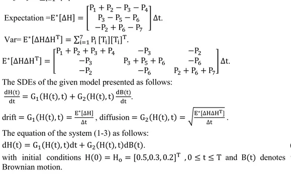
The drift and diffusion of stochastic heavy alcohol model is defined as E∗[∆H] = ∑ P i 7 i=1 Ti. Expectation =E∗[∆H] = �P1P+ P2− P3− P4 3− P5− P6 −P2+ P6− P7 � ∆t. Var= E∗[∆H∆HT] = ∑ P i 7 i=1 [Ti][Ti]T. E∗[∆H∆HT] = �P1+ P2−P+ P3+ P4 −P3 −P2 3 P3+ P5+ P6 −P6 −P2 −P6 P2+ P6+ P7 � ∆t. The SDEs of the given model presented as follows:
dH(t) dt = G1(H(t), t) + G2(H(t), t) dB(t) dt . drift = G1(H(t), t) =E ∗[∆H] ∆t , diffusion = G2(H(t), t) = � E∗[∆H∆HT] ∆t .
The equation of the system (1-3) as follows:
dH(t) = G1(H(t), t)dt + G2(H(t), t)dB(t). (4)
with initial conditions H(0) = Ho= [0.5,0.3, 0.2]T , 0 ≤ t ≤ T and B(t) denotes the
Brownian motion.
3.1 Euler maruyama technique
The parameters values which are taken from Bonyah et al. [Bonyah, Khan, Okosun et al. (2019)] are employed to produce the numerical solutions of SDEs and for this purpose. This method has been discussed in Maruyama [Maruyama (1955)] and presented in Tab. 2.
Table 2: Values of Parameter Parameters Values (years) Source
𝛬𝛬 0.04 [18] µ 0.04 [18] 𝜆𝜆 DFE=0.022 DPE=0.22 [18] 𝑣𝑣 0.04 [18] 𝑏𝑏 0.03 [18] 𝜎𝜎2 0.03 [18] 𝜎𝜎 0.09 Estimated Hn+1 = Hn+ G1(Hn, t)Δt + G2(Hn, t)∆Bn. (5)
In Eq. (5), the time step size is presented by ‘Δt’ and ∆Bn is standard normal distribution,
i.e., ∆Bn~N(0, 1). The answer of system (1) i.e., DFE is A1= (Λµ, 0,0) and the solution
4 Parametric noise in heavy alcohol model
In this way, we have chosen the parameter from the system (1-3) with minor noise as λdt = λdt + σdB. So, the stochastic epidemic of the system (1-3) is as follows [Allen and Burgin (2000); Allen (2007); Allen, Allen, Arciniega et al. (2008)]
d𝑆𝑆𝑑𝑑 = (Λ + bνR − λ𝑆𝑆𝑑𝑑𝐼𝐼𝑑𝑑− µ𝑆𝑆𝑑𝑑)dt − 𝜎𝜎𝑆𝑆𝑑𝑑𝐼𝐼ddB (6)
d𝐼𝐼d= (λ𝑆𝑆𝑑𝑑𝐼𝐼𝑑𝑑− (µ + 𝜎𝜎2)𝐼𝐼𝑑𝑑)dt + 𝜎𝜎𝑆𝑆𝑑𝑑𝐼𝐼ddB (7)
dR = (𝜎𝜎2𝐼𝐼𝑑𝑑− bvR − µR)dt (8)
In systems (6-8) of equations, randomness is presented by σ, and the Brownian motion is represented by Bk(t), (k = 1,2,3). Since the Brownian motion exists in the system (6-8),
therefore it cannot be integrated. Due to this fact, the stochastic numerical schemes will be employed in the next coming sections.
4.1 Steady state of stochastic heavy alcohol model
The stochastic models (6-7) have two steady states which are given below: Drinker-free equilibrium is A1= (Sd, Id, R) = �Λµ, 0,0�.
Drinker equilibrium is A2= (Sd, Id, R).
where,
Sd=µ+σλ2, Id=Λ+bνR−µSλSd d, R =bv+µσ2Id.
Lemma 1
For any given initial value �Sd(0), Id(0), R(0)� ∈ R+3, the solution �Sd(t), Id(t), R(t)�
of the systems (6-8) has the subsequent properties. Almost sure.
4.1.1 Stochastic Reproductive dynamics Extinction
Definition 1.
For systems (6-8) the infected individuals Id(t) are said to be extinction if limt→∞Id(t) = 0
almost sure. Let us consider, RSo= Rod− σ 2Λ2 2µ2(µ+σ2) . Theorem. If σ2<λµ
Λ and RoS < 1, then the drinker individuals of the system (6-8) tend to zero
exponentially almost surely. Proof,
Assume that (Sd(t), Id(t), R(t)) is a solution of system (6-8) satisfying the initial value
f(Id) = ln(Id) dln(Id) = f′(Id)dId+12f′′(Id)Id2�σ2Sd2�dt dln(Id) =I1d[(λSdId− (µ + σ2)Id)dt + σSdIddB] −2I1dId2�σ2Sd2�dt dln(Id) = �λSd− (µ + σ2)�dt + σSddB −12σ2Sd2dt dln(Id) = �λSd− (µ + σ2) −21σ2Sd2� dt + σSddB lnId(t) = lnId(0) + ∫ �λS0t d− (µ + σ2) −12σ2Sd2� dt + ∫ σS0t ddB where, M1(t) = ∫ σS0t ddB , with M1(0) = 0. If σ2>λµ Λ lnId≤ �λ 2 2σ2− (µ + σ2)� t + M1+ lnId(0) lnId t ≤ − �(µ + σ2) − λ2 2σ2� +Mt1+lnIdt(0) if limt→∞M1 t = 0. lim t→∞sup lnId t ≤ − �(µ + σ2) − λ2 2σ2� < 0 when σ2 > λ2
2(µ+σ2) and limt→∞Id= 0 almost sure. If σ2<λµ Λ, then ln(Id) ≤ �λµΛ −σ 2Λ2 2µ2 − (µ + σ2)� t + M1+ lnId(0) lnId t ≤ (µ + σ2) � λΛ µ(µ+σ2)− σ2Λ2 2µ2(µ+σ2)− 1� + M1 t + lnId (0) t (9) lim t→∞sup lnId
t ≤ (µ + σ2)(R0s− 1), then when R0s< 1 we get limt→∞sup lnId
t < 0
⟹ limt→∞I = 0 nearly sure. RSo = Rdo− σ
2Λ2
2µ2(µ+σ2)< 1
Note that RoS is the stochastic heavy alcohol generation number. The existence or
elimination of a disease is based on this generation number. If the stochastic heavy alcohol generation number RSo= 0.3079 < 1 , then the disease will die out in the
population. If the stochastic heavy alcohol generation number RSo= 3.1364 > 1, then
the disease will endemic in the population.
4.2 Stochastic euler technique
The systems (6-8) may be written and presented in [Raza, Arif and Rafiq (2019); Arif, Raza, Rafiq et al. (2019, 2019)]
Sdn+1= Sdn+ h[Λ + bvRn− λSdnIdn− µSdn− σSdnIdnΔBn] (10)
Idn+1= Idn+ h[λSdnIdn− (µ + σ2)Idn+ σSdnIdnΔBn] (11)
Rn+1 = Rn+ h[σ
2Idn− bvRn− µRn] (12)
where h denotes the time step size and ∆Bn~N(0,1).
4.3 Stochastic runge kutta technique
The systems (6-8) may be written and presented in [Raza, Arif and Rafiq (2019); Arif, Raza, Rafiq et al. (2019, 2019)]
Stage-1 A1 = h[Λ + bvRn− λSdnIdn− µSdn− σSdnIdnΔBn] B1= h[λSdnIdn− (µ + σ2)Idn+ σSdnIdnΔBn] C1= h[σ2Idn− bvRn− µRn] Stage-2 A2= h �Λ + bv �Rn+C21� − λ �Sdn+A21� �Idn+B21� − µ �Sdn+A21� − σ �Sdn+ A1 2� �Idn+ B1 2� ΔBn�
B2= h �λ �Sdn+A21� �Idn+B21� − (µ + σ2) �Idn+B21� + σ �Sdn+A21� �Idn+ B1 2� ΔBn� C2= h �σ2�Idn+B21� − bv �Rn+C21� − µ �Rn+C21�� Stage-3 A3= h �Λ + bv �Rn+C22� − λ �Sdn+A22� �Idn+B22� − µ �Sdn+A22� − σ �Sdn+ A2 2� �Idn+ B2 2� ΔBn�
B3= h �λ �Sdn+A22� �Idn+B22� − (µ + σ2) �Idn+B22� + σ �Sdn+A22� �Idn+ B2 2� ΔBn� C3= h �σ2�Idn+B22� − bv �Rn+C22� − µ �Rn+C22�� Stage-4 A4= h �Λ + bv �Rn+C23� − λ �Sdn+A23� �Idn+B23� − µ �Sdn+A23� − σ �Sdn+ A3 2� �Idn+ B3 2� ΔBn�
B4= h �λ �Sdn+A23� �Idn+B23� − (µ + σ2) �Idn+B23� + σ �Sdn+A23� �Idn+ B3
2� ΔBn�
C4= h �σ2�Idn+B23� − bv �Rn+C23� − µ �Rn+C23��
Sdn+1= Sdn+ [A1+ 2A2+ 2A3+ A4] 6⁄ (13)
Idn+1= Idn+ [B1+ 2B2+ 2B3+ B4] 6⁄ (14)
Rn+1 = Rn+ [C
1+ 2C2+ 2C3+ C4] 6⁄ (15)
where h denotes the time step size and ∆Bn~N(0,1).
4.4 Stochastic NSFD technique
The systems (6-8) may be written and presented in [Raza, Arif and Rafiq (2019, 2019); Arif, Raza, Rafiq et al. (2019, 2019)]
Sdn+1= Sd n+hΛ+hbvRn 1+hλIdn+hµ+hσIdn∆Bn (16) Idn+1=Id n+hλSdnIdn+hσSdnIdn∆Bn 1+h(µ+σ2) (17) Rn+1 =Rn+hσ2Idn 1+hbv+hµ (18)
where h denotes the time step size and ∆Bn~N(0,1).
4.4.1 Convergence analysis
The following theorems must be satisfied for this purpose, which are given below: 4.4.2 Theorem
For any given initial value ( Sdn (0), Idn (0), Rn (0)) ∈ R3+, system (16-18) has a unique
positive solution ( Sdn , Idn , Rn) ∈ R3+ on n ≥ 0.
Almost surely. 4.4.3 Theorem
The region Ω = �( Sdn , Idn , Rn) ∈ R3+: Sdn≥ 0, Idn≥ 0, Rn≥ 0, Sdn+ Idn+ Rn≤ Λ
µ� for all n ≥ 0 is invariant for (16-18).
Proof. The systems (16-18) may written as follows:
Sdn+1−Sdn h = Λ + bvRn− λSdnIdn− µSdn− 𝜎𝜎SdnIdn∆Bn Idn+1−Idn h = λSdnIdn− (µ + σ2)Idn+ 𝜎𝜎SdnIdn∆Bn Rn+1−Rn h = σ2Idn− 𝑏𝑏𝑣𝑣𝑅𝑅𝑛𝑛− µ𝑅𝑅𝑛𝑛 Sdn+1−Sdn h + Idn+1−Idn h + Rn+1−Rn h = 𝛬𝛬 − µ(Sdn+ Idn+ Rn) �Sdn+1+Idn+1+Rn+1�−(Sdn+Idn+Rn) h = 𝛬𝛬 − µ(Sdn+ Idn+ Rn) �Sdn+1+ Idn+1+ Rn+1� = (Sdn+ Idn+ Rn) + h[𝛬𝛬 − µ(Sdn+ Idn+ Rn)]. �Sdn+1+ Idn+1+ Rn+1� ≤𝛬𝛬µ+ h �𝛬𝛬 − µ ×𝛬𝛬µ�.
�Sdn+1+ Idn+1+ Rn+1� ≤𝛬𝛬µ+ h[𝛬𝛬 − 𝛬𝛬].
�Sdn+1+ Idn+1+ Rn+1� ≤𝛬𝛬µ.
almost surely. 4.4.4 Theorem
The discrete systems (16-18) has the same steady states as that of the continuous system (4) for all n ≥ 0.
Proof. For solving the system (16-18), we get two states as follows: DFE i.e., A3 = (Sdn, Idn, Rn) = �Λµ, 0,0�. DPE i.e., A4 = (Sdn, Idn, Rn). where, Sdn=µ+σλ2,Idn=Λ+bvR n−µSdn λSdn , R =σ2Idn bv+µ Almost surely. 4.4.5 Theorem
For given n ≥ 0, the eigenvalues of the discrete system (16-18) deceits in the unit circle. Proof.
We suppose F1, F2 and F3 from the system (16-18) as follows:
F1=1+hλISdd+hΛ+hbvR+hµ+hσId∆Bn
F2=Id+hλS1+h(µ+σdId+hσS2d)Id∆Bn
F3=1+hbv+hµR+hσ2Id
The given Jacobean matrix (JM) defined as
J = ⎣ ⎢ ⎢ ⎢ ⎡∂F∂S1d ∂F1 ∂Id ∂F1 ∂R ∂F2 ∂Sd ∂F2 ∂Id ∂F2 ∂R ∂F3 ∂Sd ∂F3 ∂Id ∂F3 ∂R⎦ ⎥ ⎥ ⎥ ⎤ where, ∂F1 ∂Sd= 1 1+hλ𝐼𝐼𝑑𝑑+hµ+hσ𝐼𝐼𝑑𝑑∆Bn ∂F1 ∂Id = −ℎ(Sd+hΛ+hbvR)(𝜆𝜆+𝜎𝜎∆Bn) (1+ℎ𝜆𝜆+ℎµ+ℎ𝜎𝜎𝐼𝐼𝑑𝑑𝛥𝛥𝐵𝐵𝑛𝑛)2 , ∂F1 ∂R = hbv 1+ℎ𝜆𝜆𝐼𝐼𝑑𝑑+hµ+hσ𝐼𝐼𝑑𝑑∆Bn ∂F2 ∂Sd= ℎ�𝜆𝜆𝐼𝐼𝑑𝑑+𝜎𝜎Id∆Bn� 1+ℎ(µ+𝜎𝜎2) , ∂F2 ∂Id= 1+ℎ𝜆𝜆Sd+ℎ𝜎𝜎Sd∆Bn 1+ℎ(µ+𝜎𝜎2) , ∂F2 ∂R = 0
∂F3 ∂Sd= 0, ∂F3 ∂Id= ℎ𝜎𝜎2 1+ℎ𝑏𝑏𝑏𝑏+ℎµ, ∂F3 ∂R = 1 1+ℎ𝑏𝑏𝑏𝑏+ℎµ.
So, the linearization of model for drinking free equilibrium A1 = (Sd, Id, R) = �𝛬𝛬µ, 0,0�
and RSo< 1.
The given Jacobean is
J = ⎣ ⎢ ⎢ ⎢ ⎢ ⎡ 1 1+hµ −h�Λµ+hΛ�(λ+σ∆Bn) (1+hµ)2 hbv 1+hµ 0 1+hλ Λ µ+hσ Λ µ∆Bn 1+h(µ+σ2) 0 0 ℎσ2 1+hbv+hµ 1 1+hbv+hµ⎦ ⎥ ⎥ ⎥ ⎥ ⎤
The eigenvalues of the Jacobian matrix is λ1=1+hµ1 < 1, λ2 =
1+hλΛµ+hσΛµ∆Bn
1+h(µ+σ2) < 1, Ro
S < 1
λ3=1+hbv+hµ1 < 1
This is guaranteed to the fact that all eigenvalues lie in the unit circle. So, the systems (16-18) is linearizable about A1.
4.5 Numerical experiments
By using the values of parameters given in the [Bonyah, Khan, Okosun et al. (2019)] the numerical simulation is discussed as follows:
4.5.1 Euler maruyama technique
The results for aforesaid technique as follow:
(c) (d)
Figure 2: (a) Susceptible heavy alcohol drinkers at h=0.01 (b) Susceptible heavy alcohol drinkers at h=2 (c) Heavy alcohol drinkers at h=0.01 (d) Heavy alcohol drinkers at h=2 4.5.2 Stochastic euler technique
The results for the systems (10-12) as follow:
(a) (b)
(c) (d)
Figure 3: (a) Susceptible heavy alcohol drinkers at h=0.01 (b) Susceptible heavy alcohol drinkers at h=4 (c) Heavy alcohol drinkers at h=0.01 (d) Heavy alcohol drinkers at h=4
4.5.3 Stochastic runge kutta technique The results for systems (13-15) as follow:
(a) (b)
(c) (d)
Figure 4: (a) Susceptible heavy alcohol drinkers at h=0.01 (b) Susceptible heavy alcohol drinkers at h=5 (a) Susceptible heavy alcohol drinkers at h=0.01 (b) Susceptible heavy alcohol drinkers at h=5
4.5.4 Stochastic NSFD technique
The results for systemS (16-18) as follow:
(c) (d)
Figure 5: (a) Susceptible heavy alcohol drinkers at h=0.01 (b) Susceptible heavy alcohol drinkers at h=100 (c) Heavy alcohol drinkers at h=0.01 (d) Heavy alcohol drinkers at h=100 4.5.5 Comparison section
The proposed stochastic nonstandard finite difference scheme and existing stochastic explicit scheme will be discussed in this section.
(a) (b)
(e) (f)
Figure 6: Contrast in results of stochastic NSFD with stochastic explicit methods, deterministic and its mean (a) Heavy alcohol drinkers at h=0.01 (b) Heavy alcohol drinkers at h=2 (c) Heavy alcohol drinkers at h=0.01 (d) Heavy alcohol drinkers at h=4 (e) Heavy alcohol drinkers at h=0.01 (f) Heavy alcohol drinkers at h=5
4.5.6 Covariance of sub-populations
For heavy alcohol epidemic model, the covariance of different sub-populations will be discussed in this section. The correlation coefficients are calculated to investigate the covariance amid distinct sub-population, and marks are described in Tab. 3.
Table 3: Correlation number
Sub-Populations Correlation Number (𝜌𝜌) Relationship
(𝑆𝑆𝑑𝑑, 𝐼𝐼𝑑𝑑) −0.6810 Inverse
(𝐼𝐼𝑑𝑑, R) 0.2210 Direct
(𝑆𝑆𝑑𝑑, R) −0.8647 Inverse
We can observe in Tab. 3 that there is an inverse relationship between susceptible heavy alcohol drinkers and remaining two sub-populations. The results in Tab. 3 show an inverse relationship between susceptible heavy alcohol drinkers and remaining two sub-populations. The drinking free equilibrium can be gained if there is an increase in susceptible heavy alcohol drinkers along with a decrease in remaining compartments. 5 Results and discussion
The fundamental Euler Maruyama (EM) technique converges to equilibria of the model for tiny step h=0.01. Meanwhile, the technique as mentioned earlier shows unnecessary behaviour of model as presented in Fig. 2: (b) and (d). The stochastic Euler converges to equilibria of the model for tiny step h=0.01. But the stochastic Euler procedure displays negativity and un-boundedness conduct as presented in Fig. 3: (b) and (d). The stochastic Runge kutta system converges to equilibria of the model in Fig. 4: (a) and (c) for tiny step h=0.01. In Fig. 4: (b) and (d), the stochastic Runge kutta system shows negativity and
un-boundedness. These techniques are time-dependent. But Fig. 5, proves to be always convergent and time-independent technique. In Fig. 6, we have presented the effectiveness of the proposed technique with other time-dependent techniques.
6 Conclusion and future framework
We can conclude that deterministic analysis of heavy alcohol model is not consistent methodology as related to the stochastic analysis of heavy alcohol model. When the time step size is very small, then the explicit numerical schemes behave well, but there is the probability that it may diverge at some particular values of time step size; also the fundamental properties of a continuous dynamical system may be loosed.
In the stochastic framework, circumscribed by Mickens [Mickens (1994, 2005, 2005)] stochastic NSFD conserves the imperative properties such as dynamical consistency and positivity.
Our keen interest in the future will be to apply the stochastic NSFD scheme to sophisticated stochastic diffusion and stochastic delay epidemic models. Furthermore, the recommended numerical analysis of this work may be used to enhance the fractional-order dynamical system [Baleanu, Jajarmi, Bonyah et al. (2018); Jajarmi and Baleanu (2018); Singh, Kumar and Baleanu (2019)].
Acknowledgement: The authors are grateful to Vice-Chancellor, Air University, Islamabad for providing an excellent research environment and facilities. The first author also thanks Prince Sultan University for funding this work through research-group number RG-DES2017-01-17.
Declaration of Conflicting Interests: The author(s) declared no potential conflicts of interest concerning the research, authorship, and publication of this article.
References
Agusto, F. B.; Okosun, K. O. (2010): Optimal seasonal biocontrol for eichhornia crassipes. International Journal of Biomathematics, vol. 3, no. 3, pp. 383-397.
Allen, E. (2007): Modeling with Ito Stochastic Differential Equations. Springer Dordrecht, Netherlands.
Allen, E. J.; Allen, L. J. S.; Arciniega, A.; Greenwood, P. E. (2008): Construction of equivalent stochastic differential equation models. Stochastic Analysis and Applications, vol. 26, no. 2, pp. 274-297.
Allen, L. J.; Burgin, A. (2000): Comparison of deterministic and stochastic sis and sir models in discrete time. Mathematical Biosciences, vol. 163, no. 1, pp. 1-33.
Arif, M. S.; Raza, A.; Rafiq, M.; Bibi, M. (2019): A reliable numerical analysis for stochastic hepatitis B virus epidemic model with the migration effect. Iranian Journal of Science and Technology, Transaction A, vol. 43, no. 5, pp. 1-18.
Arif, M. S.; Raza, A.; Rafiq, M.; Bibi, M.; Fayyaz, R. et. al. (2019): A reliable stochastic numerical analysis for typhoid fever incorporating with protection against fever. Computers Materials and Continua, vol. 59, no. 3, pp. 787-804.
Baleanu, D.; Jajarmi, A.; Bonyah, E.; Hajipour, M. (2018): New aspects of poor nutrition in the life cycle within the fractional calculus. Advances in Difference Equations, vol. 18, no. 2, pp. 1684-1698.
Benedict, B. (2007): Modeling alcoholism as a contagious disease: how infected drinking buddies spread problem drinking. Society for Industrial and Applied Mathematics, vol. 40, no. 3, pp. 1-3.
Blum, L. N.; Nielsen, N. H.; Riggs, J. A. (1998): Alcoholism and alcohol abuse among women: report of the council on scientific affairs. Journal of Women’s Health, vol. 7, no. 7, pp. 861-871.
Bonyah, E.; Khan, M. A.; Okosun, K. O.; Gomez, A. J. F. (2019): Modelling the effects of heavy alcohol consumption on the transmission dynamics of gonorrhea with optimal control. Mathematical Biosciences, vol. 309, no.1, pp. 1-11.
Chavez, C, C.; Huang, W.; Li, J. (1996): Competitive exclusion in gonorrhea models and other sexually transmitted diseases. Society for Industrial and Applied Mathematics, vol. 56, no. 2, pp. 494-508.
Chen, C. Y.; Storr, C. L.; Anthony, J. C. (2009): Early-onset drug use and risk for drug dependence problems. Addictive Behaviors, vol. 34, no. 3, pp. 319-322.
Jajarmi, A.; Baleanu, D. (2018): A new fractional analysis on the interaction of HIV with CD4+ T-cells. Chaos, Solitons & Fractals, vol. 113, no. 1, pp. 221-229.
Maruyama, G. (1955): Continuous markov processes and stochastic equations. Rendiconti Del Circolo Matematico Di Palermo, vol. 4, no.5, pp. 48-90.
Mickens, R. E. (1994): Nonstandard Finite Difference Models of Differential Equations; World Scientific, Singapore.
Mickens, R. E. (2005): A fundamental principle for constructing nonstandard finite difference schemes for differential equations. Journal Difference Equations and Applications, vol. 11, no. 7, pp. 645-653.
Mickens, R. E. (2005): Advances in Applications of Nonstandard Finite Difference Schemes; World Scientific, Hackensack.
Raza, A.; Arif, M. S.; Rafiq, M. (2019): A reliable numerical analysis for stochastic dengue epidemic model with incubation period of virus. Advances in Difference Equations, vol. 3, no. 2, pp. 1958-1977.
Raza, A.; Arif, M. S.; Rafiq, M. (2019): A reliable numerical analysis for stochastic gonorrhea epidemic model with treatment effect. International Journal of Biomathematics, vol. 12, no. 6, pp. 1-26.
Room, R.; Babor, T.; Rehm, J. (2005): Alcohol and public health. The Lancet, vol. 365, no. 5, pp. 519-530.
Saunders, J. B.; Aasland, O. G.; Amundsen, A.; Grant, M. (1993): Alcohol consumption and related problems among primary health care patients: who collaborative project on early detection of persons with harmful alcohol consumption. Addiction, vol. 88, no. 3, pp. 349-362.
Singh, J.; Kumar, D.; Baleanu, D. (2019): New aspects of fractional biswas milovic model with mittag leffer law. Mathematical Modeling of Natural Phenomena, vol. 14, no. 3, pp. 01-18.
Testino, G. (2008): Alcoholic diseases in hepato-gastroenterology a point of view. Hepatogastroenterology, vol. 55, no. 83, pp. 371-377.
Walter, H.; Gutierrez, K.; Ramskogler, K.; Hertling, I.; Dvorak, A. et al. (2003): Gender specific differences in alcoholism implications for treatment. Archives of Women’s Mental Health, vol. 6, no. 4, pp. 253-258.